Drone operational settings such as capacity, speed, and swath width are useful figures for calculating productivity, but they only describe the airborne portion of the job. A commercial application business must also transport water, mix product, charge batteries, and establish an efficient staging area that is both safe for operators and maintains drone connectivity. If any of these functions fall behind, productivity suffers.
We consulted several mission records to develop a productivity calculator that can model a range of scenarios. We assumed a shuttle (back-and-forth) flight pattern to apply successive spray swaths for uniform coverage of a treatment area.
How to use
In this, version 4.0 of our drone productivity calculator, we’ve expanded the functionality to include several tendering options. If you are uncertain what the variables mean, consult this handy instruction manual to walk you through the process.
Use it as a planning tool, or simply as a way to explore the impact of different operational settings on mission productivity. We propose adjusting variables one at a time to determine their effect. You can then compound the effect by changing another, or return to the base value and choose another variable to manipulate. In this way you can explore the relative influence of each variable on the overall job.
Which factors matter most?
The relative impact of each operational setting (or the geometry of the target area) on productivity is situation-specific. Nevertheless, here are some generic observations:
While swath width and flight speed play a role, both are limited by the agronomic realities of the job. So, while you can change them in the calculator, it does not follow that the results of the application will be successful.
Water rate (e.g. L/ha) has an impact on productivity, but once again there are agronomic considerations. Too low a volume can compromise product efficacy and contribute to off target drift, and quite often the minimum volume is stipulated on the product label.
The drone’s tank capacity depends on the model, but maxing it out may not be the best option. Some large drones suffer reduced battery life and slower acceleration when filled completely. Note that when the user forces a refill/battery swap, there will be spray mix left in the drone. It is prudent to minimize this residual by not overfilling the drone in the first place.
The ferrying distance between where the drone empties and the staging area a critical productivity factor, so minimizing it is a reasonable objective. Doing so can mean additional sorties, which require additional refills and battery swaps. Small improvements here compound into big impacts, but pay close attention to see if the additional sorties are worth the time savings.
The number of operators have a significant effect on productivity. If a solo operator has to retrieve additional water, or move the tender truck to a new location, the drone isn’t spraying.
Batteries – A potentially limiting factor
The calculator assumes that a sufficiently charged battery is ready whenever the drone returns to the tender, so battery charging does not extend the entered refill and battery-swap time.
In practice, flight endurance can change dramatically with payload. For example, a heavily loaded aircraft may fly for only a few minutes, while the same aircraft may remain airborne much longer with an empty tank. Repeated short, high-load sorties may therefore consume charged batteries faster than they can be recharged.
If the battery inventory, chargers, generator capacity or electrical supply cannot keep pace, the crew may eventually have to wait for batteries, reducing actual productivity below the calculator’s estimate. Additional batteries, higher-capacity charging equipment or improved generator capacity may be required to sustain the projected workflow.
Thanks to Mike Verhoog (Drone Spray Canada) and Dr. Michael Reinke (Michigan State) for discussions contributing to the design of this model.
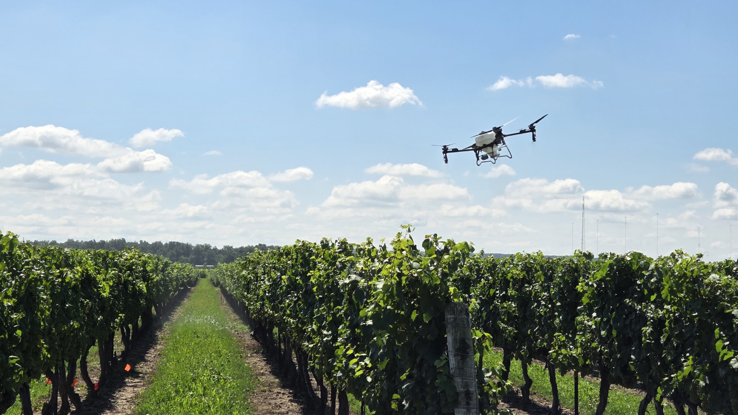
In this study, 3D sampling of drone spray applications in wheat demonstrates that coverage is strongly influenced by the interaction between drone downwash, flight speed, and wind conditions. These factors collectively determine where droplets land, how evenly they are distributed, and how reliable coverage is from pass to pass. In 2025 we characterized wheat head coverage from a DJI Agras T50. In this study, we explore the larger, faster DJI Agras T100, and relate the observations to what we’ve seen in previous studies.
Materials and Methods
Site and crop
The experiment was conducted at 45939 John Wise Line, St. Thomas, Ontario (42°43’57.0″N, 81°05’49.8″W) on June 3, 2025. Wheat was seeded at 1.8 million seeds/ac on 19 cm spacing and was at the T3 stage (~0.7 m height) at application.
Design
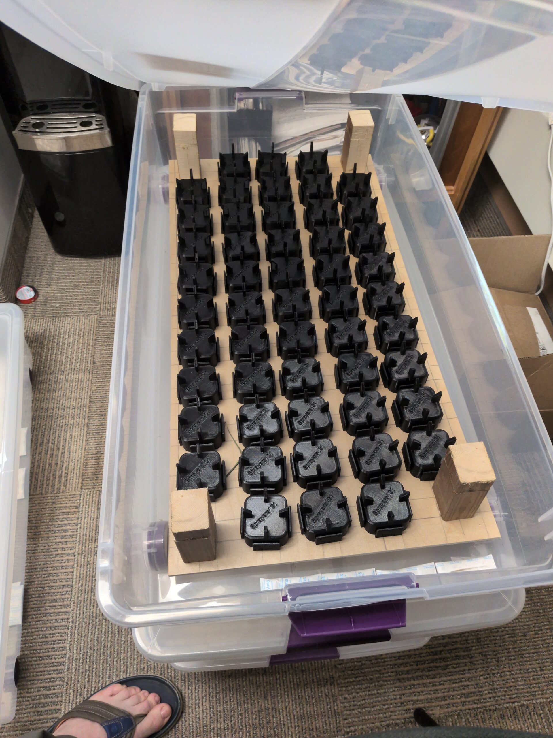
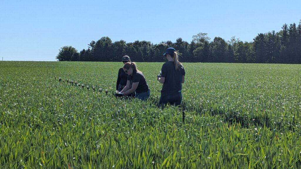
Twenty-one poles spaced at 1 m intervals held 3D-printed mounts with 1×3″ water-sensitive papers oriented in four directions relative to the drone flight path: advance, retreat, left, and right. A tramline behind the array preserved canopy structure while allowing access to the samplers (Figure 1).
Figure 1 – Volunteers retrieving and replacing samplers between passes.
Drone Operational Settings
The primary objective of the study was to explore the effect of flight speed on coverage. Speed was increased from 6, to 10, to 14 m/s with the following operational settings:
4 LX07550SX (sprinkler) nozzles
50 L/ha application volume
350 µm droplet size
4 m flight altitude
7 m programmed swath width
Tank volume maintained at ~50 L
The drone began spraying 50 m before and continued 20 m after the samplers, flown on full auto over pole 10 and 11 (the middle of the 21 poles). The spray liquid was municipal water with 0.5% v/v of MasterLock (Winfield United).
The secondary objective was to compare coverage from the drone spraying 5 gpa (6 m/s) to a 10 gpa (7 m/s) condition.
Weather
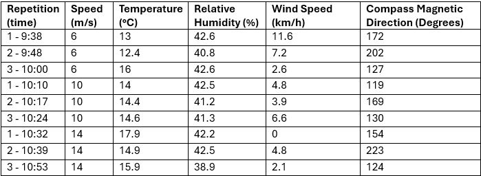
Weather data was collected using a Kestrel 3550AG weather meter (Kestrel Instruments) in a vane mount positioned roughly 2 m below drone altitude. Data was logged as the drone passed the samplers (Table 1).
Table 1 – Weather conditions for each spray pass.
Flights were conducted under a prevailing tailwind (rather than the preferred headwind) due to field constraints. Wind conditions during application varied by treatment. The 6 m/s treatment experienced higher and more variable wind speeds (avg. 6.6 km/h, SD 3.7 km/h, 177°), predominantly from the north (tailwind). The 10 m/s treatment occurred under moderate and stable winds (avg. 4.8 km/h, SD 1.1 km/h, 136°) with a slight right-to-left crosswind component. The 14 m/s treatment experienced low and variable wind speeds (avg. 1.6 km/h, SD 2.0 km/h, 198°) including periods of calm .
Results
Deposition Magnitude and Orientation
Papers were analyzed using a DropScope™ (SprayX, São Carlos, Brazil). Deposition differed strongly by collector orientation (Table 2). Some repetitions were removed if wind pushed spray beyond the collectors. This left a minimum 2 repetitions per condition.
Speed
Direction
Mean(deposits/cm2)
Std Dev
Min
Max
6 m/s
Advance
45.70
67.03
1.3
210.7
Left
40.06
66.19
0.0
211.8
Retreat
20.10
20.25
0.0
71.0
Right
45.47
73.55
0.0
208.9
10 m/s
Advance
52.07
63.05
0.1
189.3
Left
31.95
43.65
0.0
136.0
Retreat
5.12
9.19
0.0
37.6
Right
37.22
70.18
0.0
202.1
14 m/s
Advance
39.02
37.51
0.5
115.3
Left
26.89
43.91
0.0
130.9
Retreat
0.43
1.27
0.0
5.7
Right
11.03
22.53
0.0
71.2
Table 2 – Average deposition by sampler orientation for each speed.
Forward-facing collectors (advance) consistently recorded the highest deposition across all speeds, followed by lateral orientations. Reverse-facing collectors (retreat) recorded substantially lower deposition. Variability was high for advance and lateral orientations, whereas retreat collectors showed consistently low variability (Table 3).
Direction
Mean(deposits/cm2)
Std Dev
Min
Max
Advance
39.02
37.51
0.5
115.3
Left
26.89
43.91
0.0
130.9
Retreat
0.43
1.27
0.0
5.7
Right
11.03
22.53
0.0
71.2
Table 3 – Average deposition by sampler orientation for all passes.
Directional Bias (Anisotropy)
Anisotropy refers to the property of having different values when measured in different directions. We can quantify this by dividing the average coverage on one plane by the opposite plane; The resulting indices show the relative direction of deposition.
For the lateral plane (left-to-right), we divide the average coverage on the left-facing orientation by the right. On the sagittal plane (advance-to-retreat), we divide the average coverage on the advance-facing orientation by the retreat (Table 4).
Speed
Lateral (L÷R)
Sagittal (A÷R)
6 m/s
0.88 (slight right-dominant)
2.27 (moderate advance-dominant)
10 m/s
0.86 (slight right-dominant)
10.17 (strong advance-dominant)
14 m/s
2.44 (strong left-dominant)
90.05 (almost entirely advance-dominant)
Table 4 – Relative coverage indices for lateral and sagittal planes.
Bias in the lateral index was relatively weak, with a subtle shift with the wind (wind-facing is left) at higher speeds. The sagittal index (advance-to-retreat) increased from a 2x between 6 m/s and 10 m/s to 5x between 10 m/s and 14 m/s, demonstrating strong forward bias with flight and wind direction despite the down-and-back vector created by the downwash.
Spatial Distribution
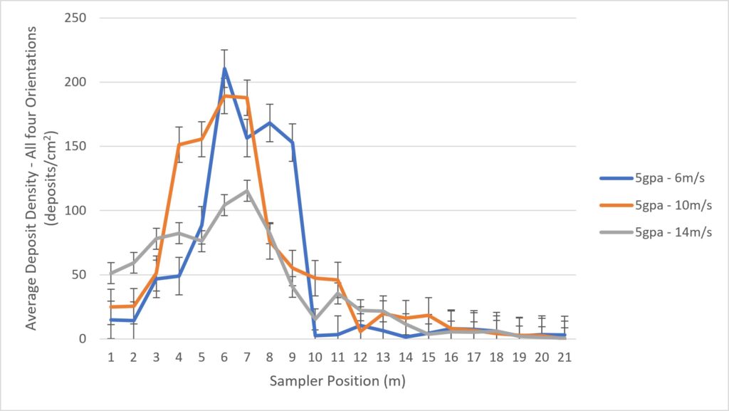
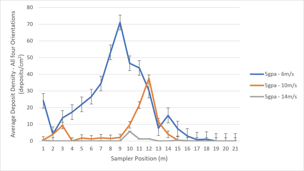
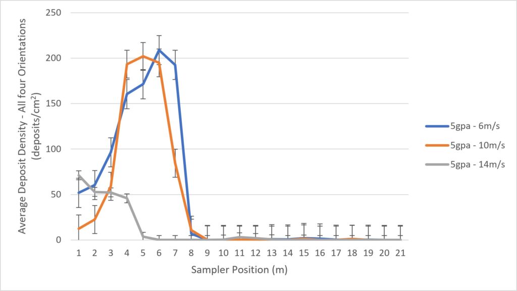
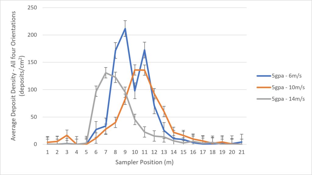
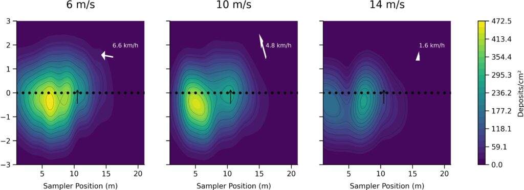
Peak deposition consistently occurred 1 to 5 m downwind of the flight line, rather than directly beneath it. A cross-tail wind shifted deposition laterally, while forward motion (inertia) and wind reinforced deposition in the advance direction. This can be illustrated by isolating the average coverage for each orientation, for all three speeds (Figures 2 to 5).
Figure 2- Advance Orientation (Facing tailwind). Bars = SEFigure 3 – Retreat Orientation (facing away from tailwind). Bars = SEFigure 4 – Right Orientation (Facing cross wind). Bars = SEFigure 5 – Left Orientation (facing away from cross wind). Bars = SE
By combining and plotting average coverage on all orientations in a top-down heatmap, we can clearly see the lateral shift to the left of the flight pass (with the light crosswind), the higher relative coverage on the advance face, and indications of bi-modal coverage that likely corresponds to the position of the rotary atomizers(Figure 6).
Figure 6 – Coverage heatmap created by smoothing the average deposition data for each speed (σ ≈ 1.1 – 1.2 m) over a 300 x 300 grid to illustrate deposition gradients. The colour scale supports a direct comparison of deposition intensity. The 21 samplers are indicated by black dots spaced at 1 m intervals, and the drone flight path appears as a black arrow between posts 10 and 11. Average wind speed and direction appears as an inset white arrow (vector).
Effect of flight speed on swath width
Swath width was determined by averaging all deposition on each post for each speed and using our online swath width calculator. The range of flight speeds used in this study did not significantly affect swath width.
6 m/s: 8 m swath width (16.3 % C.V.).
10 m/s: 7.5 m swath width (22.5 % C.V.)
14 m/s: 7.5 m swath width (22.3 % C.V.)
These widths are 15-20% wider than the widths calculated in the same manner during the 2025 study with the T50.
Averaging swath widths can mask variability
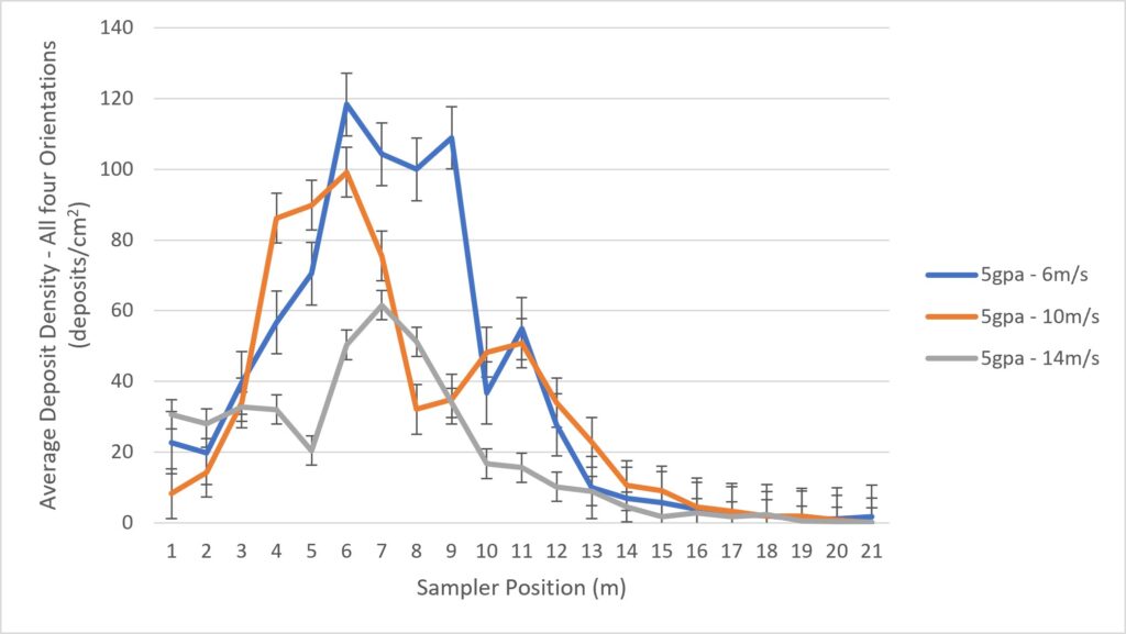
This method of calculating and comparing average swath widths is convenient, but it hides any variability in the amount of spray deposited within the swath. Consider that an 8 m swath with 10 deposits/cm2 every meter would have the same C.V. as an 8 m swath with 100 deposits/cm2. Deposit variability can be illustrated by plotting the average coverage along the swath with standard error (figure 7). We see that flight speed significantly influenced the degree of deposition, where higher speeds reduced the average droplet density (counts) as well as the variability (standard deviation).
Figure 7 – Average coverage, all orientations, for each speed. Bars = SE
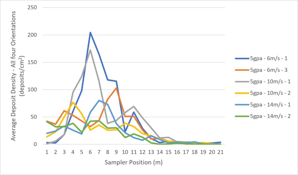
Think of each repetition as a randomly-selected cross section of the swath from somewhere along a spray pass. Calculating swath width from averaged coverage data can hide shifts in the relative position along the flight path, making the composite value greater than that of any single replicate. This variability and the potential for inadvertent smoothing can be exposed by plotting each repetition. (Figure 8).
Figure 7 – Average coverage (all orientations) from each pole plotted by speed and repetition.
Therefore, the order of operations matters. When swath width is calculated for each repetition, and then averaged, we would expect the widths to be somewhat smaller. They are presented here in table form next to the previous values for comparison (Table 5).
Speed (m/s)
(A) Deposition averaged, then swath calculated (m)
(B) Swaths calculated, then average (m)
Difference (A-B) (m)
6
8 (16.3% C.V.)
6 (29.6% C.V.)
-2
10
7.5 (22.5% C.V.)
6 (33.5% C.V.)
-1.5
15
7.5 (22.3% C.V.)
7.5 (30.5% C.V.)
0
Table 5. Average swath widths generated by two methods.
Statistical Analysis
No matter the method, we can draw conclusions from the swath widths calculated here.
6 m/s: highest deposition but greatest variability.
10 m/s: best balance of deposition, uniformity, and swath width.
14 m/s: lowest deposition and most directional bias.
A two-way analysis of variance (ANOVA) was conducted to evaluate the effects of flight speed and collector orientation on spray deposition. Deposition differed significantly between Advance, Left, Right, and Retreat collectors (F = 6.1, p = 0.0005). Flight speed had a statistically significant effect on deposition, where deposition was reduced with speed (F = 3.03, p = 0.05). The effect of orientation did not significantly depend on speed (F = 0.46, p = 0.83), suggesting that the pattern of deposition was consistent across speeds.
Effect of volume on deposition
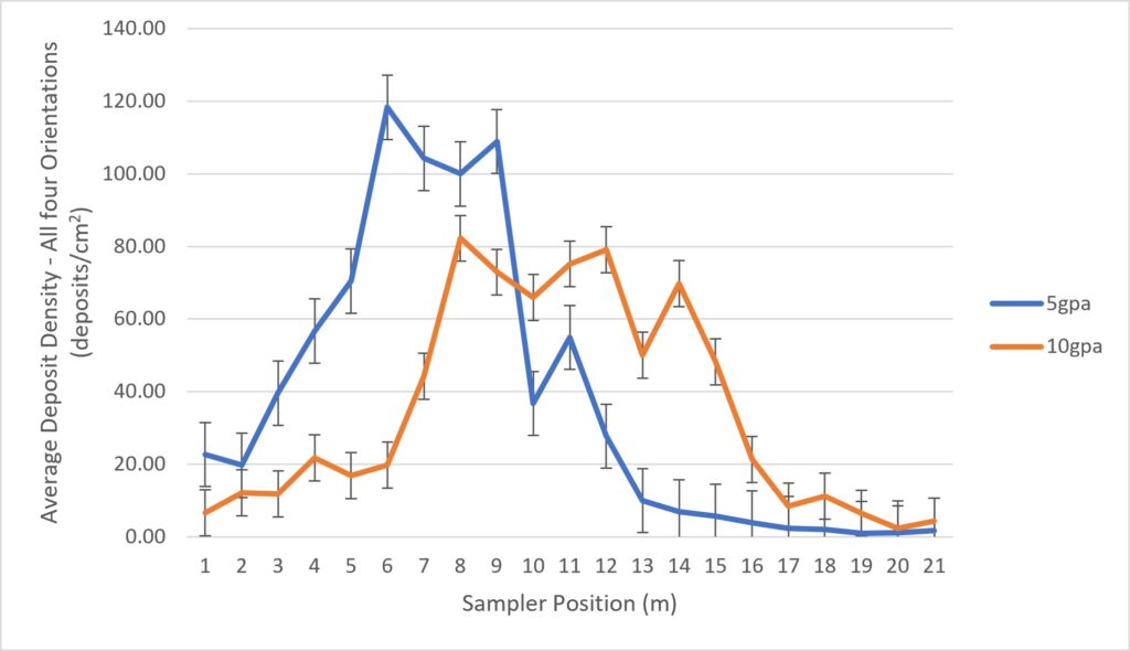
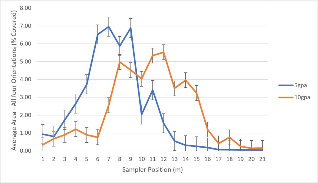
In a secondary investigation, the drone was flown at 7 m/s, applying 10 gpa to compare coverage to the 6 m/s, 5 gpa condition (Figure 8).
Figure 8 – Average coverage as deposit counts, all orientations, for 5 gpa and 10 gpa. n=2 for each condition . Bars = SE
Surprisingly, there was no significant increase in total deposition within the swath when volumes were increased. In fact, the 5 gpa condition is ~8% higher when all deposits are summed or when area under the curve is calculated. The relative shape of the curve was notably different with 5 gpa producing a sharper, higher-intensity central peak, while 10 gpa produced a broader and more uniform deposition profile.
It was expected that higher volumes would result in higher counts. One theory for the absence of this result was that overlapping depositions in the high volume treatment might have underestimated counts when the papers were digitized. Therefore, the percent surface area was also analyzed (Figure 9). Once again, there was no significant difference in the total percent area or a comparison of area under the curves.
Figure 9 – Average coverage as area covered, all orientations, for 5 gpa and 10 gpa. n=2 for each condition . Bars = SE
When swath widths were calculated for each repetition, then averaged for each speed, we arrived at (5 m + 7 m) ÷ 2 = 6 m for the 5 gpa condition, and (5.5 m + 6.5 m) ÷ 2 = 6 m for the 10 gpa condition. We have no explanation for why there was no volume-related difference.
Discussion
Wind direction strongly influenced deposition, overriding the down-and-back pattern seen in previous studies. A tail-cross wind likely drove deposition (likely occurring after the drone passed the sampling location), explaining why retreat-facing collectors captured minimal deposition, and peak deposition was accordingly displaced from the flight line.
Overall, results confirm that wind conditions fundamentally reshape spray distribution. The implication is that wind direction must be accounted for alongside swath width when developing flight path spacing to minimize the potential for overlaps and gaps between passes.
Further, previous studies have demonstrated a direct and positive relationship between flight speed and swath width up to 8-10 m/s with no further response after ~8 m/s. This study supports the hypothesis that rotary-wing drone speed and swath width share an asymptotic relationship that inflects at ~8-10 m/s (variability makes it difficult to determine an exact value). Flight speed also has a direct and inverse impact on the degree of spray deposition and deposit variability within the swath.
Finally, caution is advised when interpreting average swath widths. There may be no indication of the degree of coverage within the swath (affecting efficacy), or the lateral variability along the flight path (affecting fieldwide uniformity).
Related video
Thanks to Adam Pfeffer and Bayer Canada for in kind and financial support, and thanks to volunteers Erin Jewson (OMAFA Engineer), Halle Barton and Nikki Intranuovo (Bayer Summer Students) for their help with the field work.
Author’s Note: These results were adjusted in July to exclude outliers and include the results of the spray volume comparison.
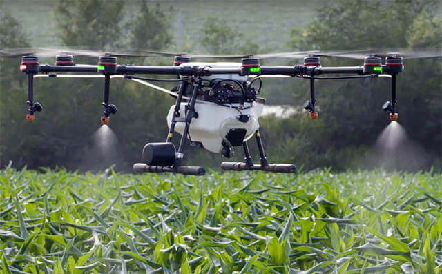
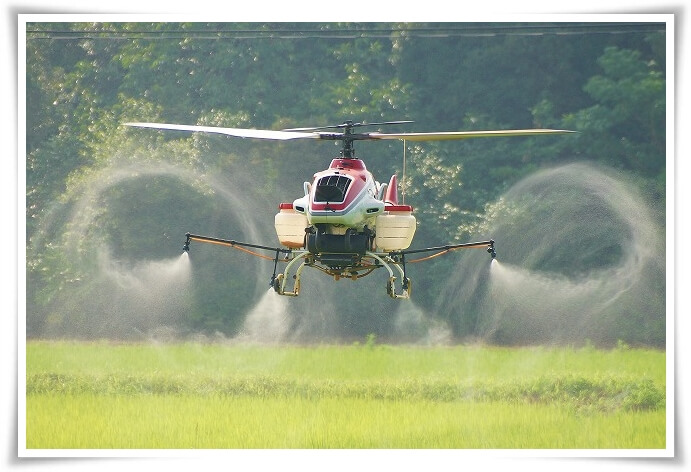
Spray application by drone is here. It’s common practice in South East Asia, with a very significant proportion of ag areas now treated that way. Estimates from South Korea, for example, suggest about 30% of their ag area being sprayed by drone. It’s in the US, too. The Yamaha RMax and Fazer helicopters, which pioneered drone spraying in Japan dating back to the mid 1990s, have been approved for use in California since 2015. DJI, the world’s largest drone manufacturer, introduced their ag model, the Agras MG-1, to North America in 2016. Many other spray drones are available or in development.
As William Gibson, the author of Johnny Mnemonic, once said,
“The future’s here, it’s just not widely distributed yet.”
DJI Agras MG-1 spray drone (Source: DJI.com)
Proponents of drone spraying cite a drone’s ability to access areas where topography is a problem, such as steep slopes, where productivity of manual application is much lower, or low areas where soil moisture prevents ground vehicles. Operator exposure is reduced compared to handheld application.
Opponents talk about productivity and cost factors compared
to manned aerial application, spray drift, and rogue use.
Before drone spraying becomes commonplace, two important
things need to happen.
Federal laws need to be updated to accommodate the unique features of remotely piloted aircraft systems (RPAS), as they’re now called. Current laws make many assumptions unique to manned ships, and the process to correct that will require some patience. A thorough review for US laws, and their shortcomings, can be found here.
Federal pesticide labels need to permit the use of drones for application. As of August, 2021, Canadian labels have no such registered use.
There is no doubt that we need to prepare for a future that includes spraying by drones. Features such as topography adjustment for height consistency and autonomous swath control are already essentially standard, and the capabilities that improve control and safety will continue to develop.
And yet I’ve been nervous about the prospect of pesticide application with drones. My primary concern is around – you guessed it – spray drift. Because a drone payload is relatively small (about 5 to 25 L, depending on the model), application volumes will need to be low to have any sort of productivity. How low? For manned aircraft with a 200 to 600 gallon hopper, 2 to 4 US gpa (18 to 36 L/ha) are the lowest commonplace volumes. The lower volumes require a Medium spray quality (among the finer sprays in modern boom spray practice) to achieve the required coverage.
It’s a simple concept: the less water is used, the smaller the droplets need to be to provide the necessary droplet density on the target. Drift control with coarser sprays requires higher volumes, and true droplet-size-based low-drift spraying can’t really happen at volumes less then, say 5 to 7 US gpa.
At 2 to 4 US gpa, a drone would be able to do perhaps 1 acre per load. While OK for spot spraying, it represents a serious productivity constraint for anything larger. There will be a push toward lower volumes, perhaps 0.5 to 1 gpa (5 to 10 L/ha). The only way these will provide sufficient coverage is with finer sprays, ASABE Fine to Very Fine, with expected problematic effects on off-target movement and evaporation. These fine droplets are also more prone to the aerodynamic eccentricities of aircraft.
Vortices from the rotor can create unpredictable droplet movement (Source: kasetforward.com)
The current regulatory models for aerial drift assessment in North America, AgDISP and AgDRIFT, are not yet able to simulate drone application. But by entering finer sprays into these models for their conventional manned rotary wing aircraft, we can see that buffer zones will be higher. Much higher. And that outcome will give pause to regulators. Failure to control the movement of a spray is, and should be, a problem.
Estimated Buffer Zones (calculated by AgDISP) for a reference rotary wing spray aircraft, using three pesticide toxicologies and two spray qualities.
Furthermore, ultra-low volume (ULV) sprays can change the efficacy of some products, and these will require new performance studies. At this time, regulators are seeking information not just on spray drift, but on product efficacy, operator and bystander exposure, and crop residues.
Regulators are currently collecting spray drift and efficacy data from drones. Since the drones available in today’s market do not conform to a common design standard like fixed or rotary winged manned aircraft, each model may have its own characteristics and need its own study. Some will have rotary atomizers, others will use hollow cone hydraulic sprays. Some will have electrostatic charging, others may propose special adjuvants.
Once data are assessed, there will likely be restrictions in flight height, flight speed, wind speed, spray quality, water volume, perhaps air temperature and relative humidity (or Delta T). This is not new to spraying, as current labels already constrain use for both ground and aerial spray application, more so for aerial.
The obvious question is how these proper application practices can possibly be assured. Operators will need more than just regulatory approval to use a drone, they will require proper training, similar to what a commercial aerial applicator now receives prior to operating a business.
Recall that our aerial applicators are governed by national organizations, the NAAA in the US and the CAAA in Canada. These organizations are in regular contact with federal regulators to assure compliance. They also help fund research into application efficacy and safety. They organize conferences in the off-season and calibration clinics in the growing season. At these, flow rates are confirmed and deposited droplet size is measured. Spray pattern uniformity is assessed and corrected as necessary.
Should drone applications be exempt from these controls? I don’t think that would be wise. Are we ready to implement them? Absolutely not.
These requirements would change the drones’ economic model. And despite these precautions, a drone may still leave the control of a pilot due to unforeseen technical or human events.
In the US, Yamaha does not sell their drone helicopters. Instead, they deploy their own teams to make the applications. This way, they have assurance that only trained and experienced pilots use the technology.
As the industry gears up for the first registrations, we see drone service companies take a leading role in testing. Much is being learned via legal applications of liquid micronutrients, for example, or limited use of pesticides under approved research permits. And I’m pleased to see the recognition of drift management in these efforts through the use of low-drift nozzles. We are off to a promising start.
Requests for drone use are in progress at our regulatory agencies. The outcomes of their risk assessments will provide important initial guidance, and food for thought and discussion. In the meantime, the drone development continues at a rapid pace, with new features and greater capacity at each iteration.