Tag: uniformity

  • What’s the Cost of Poor Deposit Uniformity?

    What’s the Cost of Poor Deposit Uniformity?

    We’ve heard it often: calibrate your nozzles to be sure your boom output is uniform across its entire width. The downside of poor uniformity is obvious: strips of over- or under-application causing problems with pest control or crop tolerance. A graduated cylinder held for 30 s under each nozzle is the approach of choice. Several electronic versions exist to make the job easier, for example the Spot On.

    But there’s more to the story. Nozzle calibration only ensures volumetric uniformity from nozzle to nozzle. It serves to identify worn, plugged, or damaged nozzles, and little else.

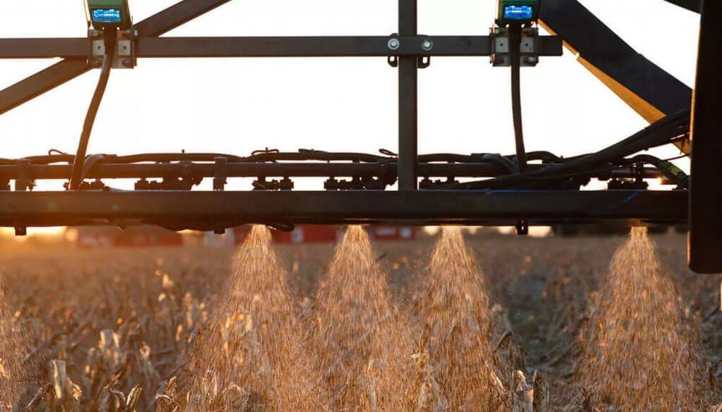
    After release, the spray is atomized and distributed across a wider area with a properly developed pattern. An operator adjusts boom height or spray pressure to generate proper overlap for a given fan angle at the target height. Unfortunately, the uniformity of this pattern can’t be measured with a graduated cylinder, so we’ve traditionally used a “patternator”, a flat collector placed under a few nozzles that uses a series of channels to show the peaks and valleys of the volumetric distribution. Both calibration and patternation are done with a stationary spray boom. Nozzle manufacturers employ both methods to ensure their products meet international uniformity standards before marketing.

    A spray patternator determines the uniformity of a stationary boom’s spray distribution (Photo: TeeJet)

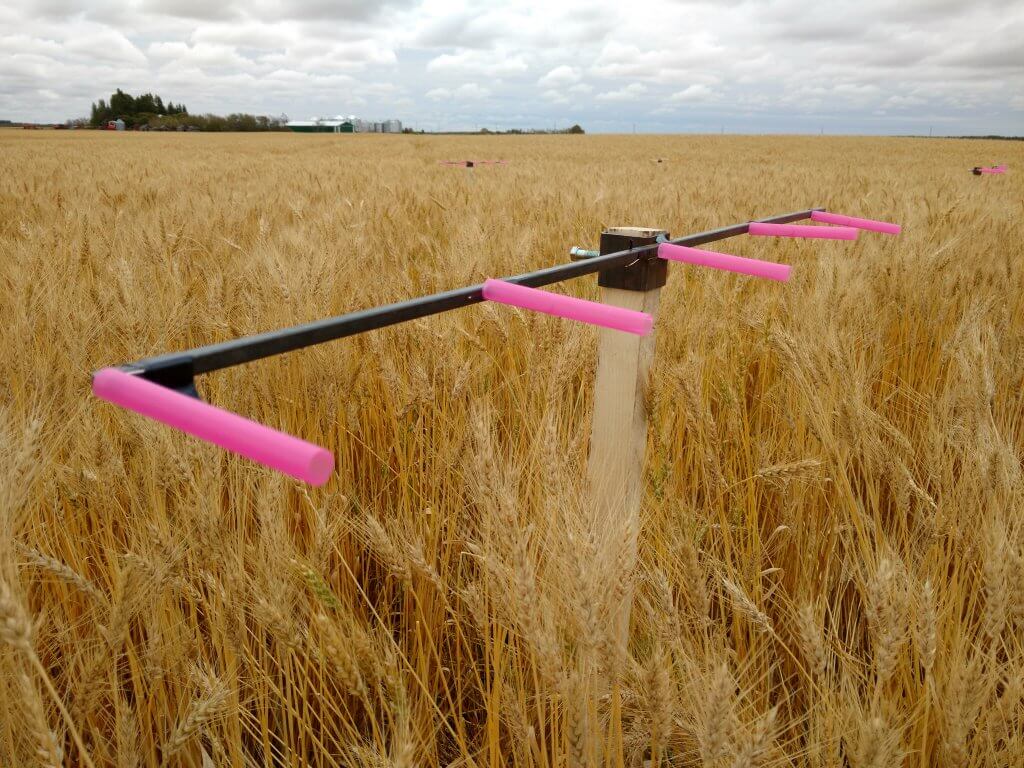
    Burt even that isn’t enough. We can have good volumetric distribution but still have inconsistent coverage in places. To identify those regions, we need a way to measure small amounts of spray deposit under a moving boom, ideally in the canopy we intend to treat. Here we have a few options. We can place a tracer (dye, salt, etc.) in the tank, and collect spray on small collectors placed throughout the area to be treated. We collect the samples, wash them, and analyze the solvent for the tracer. This requires special equipment and takes time. It’s useful, but only measures dose, not droplet size or density.

    Plastic straws can act as collectors of sprays under field conditions.
    Monofilament strings can be used to collect spray over long distances.

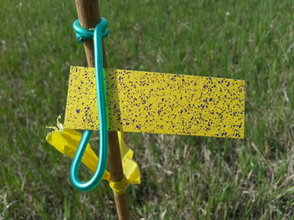
    A faster way is to use water-sensitive paper, about which we’ve written here and here. Using WSP is fast and easy, and it can provide additional information such as the number of droplets per unit area, or the total percent of the area covered, or even the size of the deposits, with the right equipment. We call this “coverage”, and believe this to be one of the two components of good pest control (the other being “dose”, the total amount of material deposited). Because the world isn’t fair, WSP isn’t great at quantifying dose.

    Water-Sensitive paper provides a quick visual indication of the deposit, not just amount but also qualitative aspects such as droplet size and distribution.

    The industry has done a good job of identifying the dose required for good control, and this is reflected in the rate recommendations on a label. But there are a few gaps. They don’t tell us, for example, what “good coverage” is, despite often telling us to “ensure” it.

    Back to Deposit Uniformity

    We quantify deposit uniformity by calculating the Coefficient of Variation (CV) of a series of measurements. The CV is defined as the standard deviation of these measurements, expressed as a percent of the mean value.

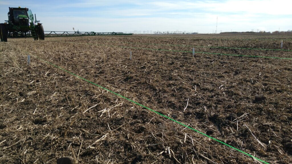
    Because it’s hard to measure, it’s easy to ignore. But here are a few basics our research has told us: (In the first three examples, deposits were measured under a spray boom using petri plate or drinking straw samplers. There was no interference from a canopy. The last example was taken from within a canopy.)

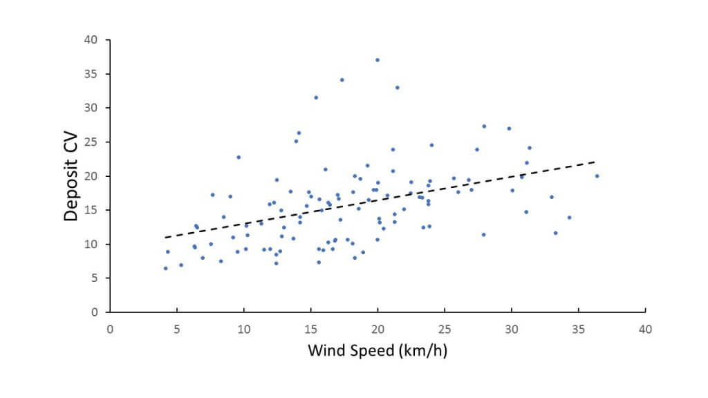
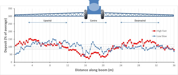
    • When measuring the deposited dose, the CV under a boom tended to rise with increased wind speed. This is no surprise, as it reflects that more wind has a greater chance to displace spray from its intended destination.
    Spray deposit uniformity, observed during various spray drift studies, tended to decrease with higher wind speeds.
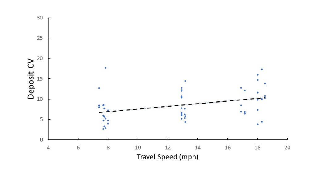
    • Higher booms and increased travel speed also tended to increase deposit CV.
    Faster travel speeds during spray drift studies tended to decrease uniformity.
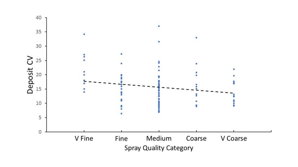
    • Finer sprays tended to increase deposit CV. This makes sense, as the finer droplets are more easily displaced by air movement.
    Coarser sprays created more uniform deposits possibly because they were more resistant to turbulent displacement.
    • Deposits were reduced and became more variable deeper in a broadleaf canopy. Again this makes sense, as there are a lot of obstacles to clear and canopies themselves are by no means uniform.
    Deposit amount was lower in the canopy, as expected. But the lower deposit was also more variable.

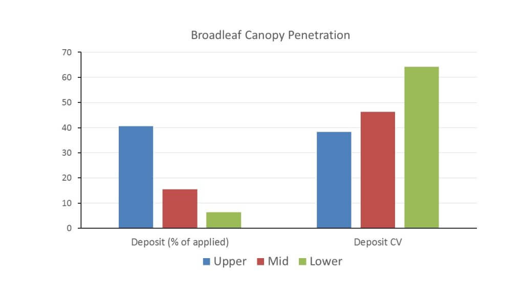
    Also note that the CV in the canopy was quite a bit higher (40 – 60%) than for the exposed targets (10 – 20%). That’s another challenge.

    To recap, the best uniformity was achieved with low booms (as long as patterns overlap sufficiently), slow speeds, low winds, and coarser sprays. It’s easy to see that current spray practice isn’t always conducive to uniform deposits.

    Deposit variability as captured by a 2 mm diameter string with two sprayer configurations.

    So What?

    Why does uniformity matter? It matters because more variable deposits are less efficient. They require higher doses for the same effect as uniform deposits. Here’s why:

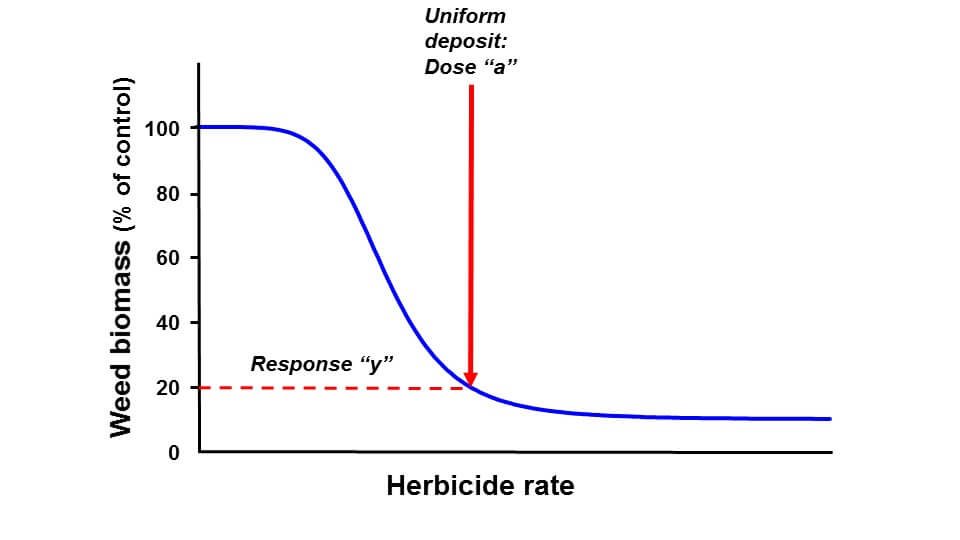
    The figure below shows a typical dose response curve for a herbicide. On the y-axis, we see weed biomass, on the x-axis herbicide dose. At low pesticide doses, not much happens. (In fact, we often see a slight increase in biomass with very low herbicide doses.) As we increase dose, biomass begins to decline, and as dose increases further, the effect begins to taper off. At a certain dose, no further biological response is possible.

    A typical dose response curve for a herbicide.

    In the next figure, we see that application of a uniform dose “a” results in biomass “y”, about 20% of untreated.

    A dose response curve represents the weed biomass that resulted from any applied dose.

    Next, we apply the same average dose, but we do it non-uniformly. At some locations under the boom, the deposit may be 40% higher or lower than average. The result is response “z”. Weed control is worse, as bad as it would have been at a lower uniformly applied dose (effective dose “b”).

    A variable dose across a field results in many individual weed biomasses because of deposit variation. The net result is lower control.

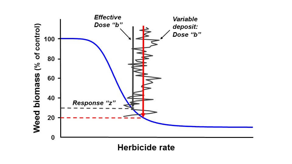
    This effect only happens when the effective dose is near the lower inflection point of the dose response curve. Perhaps we’re shaving rates. Perhaps the weather is challenging the herbicide’s performance. Or perhaps the weed is difficult to control. Under those conditions, any gain in performance with a higher dose is less than the penalty from a lower dose.

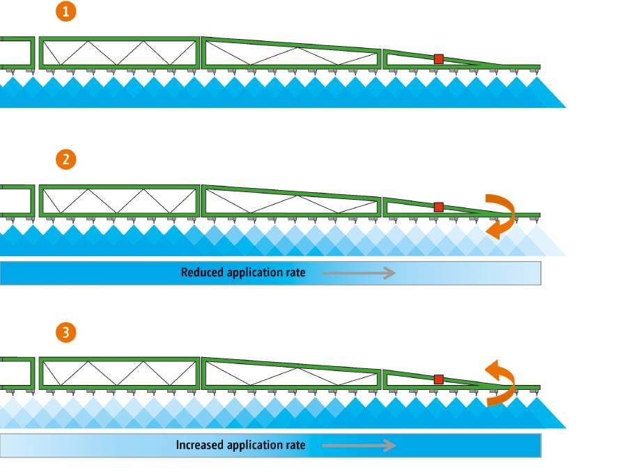
    There are two ways to correct this performance loss. One is to apply a higher herbicide rate. It’s commonly done, as insurance against – you guessed it – variability, and it’s one reason why label rates have some flexibility. The second way is to improve deposit uniformity. In effect, better uniformity allows for rate reductions.

    Label rates are typically in the flat region of the dose response curve to allow for variable conditions in weed susceptibility, weed growth stage, growing conditions, and deposit variability.

    Take Home Message

    Uniform spray deposition improves overall control. Our examples used herbicides, but the same is true for fungicides and insecticides. It’s true for field crops as well as fruit and vegetable sprays.

    Uniformity is especially important when the application is done under adverse conditions in which the pesticide performance is challenged. It’s a fundamental part of good application practice.

    It’s not always easy to improve uniformity. But at least it should be measured. Without measuring it, an applicator may never know how much product is being wasted. Have a look at the Crop Adapted Spraying approach Jason is using, it’s a template for all sorts of applications.

    What can you do? The easiest task is to record the flow from each nozzle. The results might be surprising. Ensuring proper and consistent boom height is also important. Using water-sensitive paper to visualize the quality of the job would be icing on the cake. And adjusting application method, with uniformity as a goal…that gets you a gold star.

  • Reducing Selection Pressure for Herbicide Resistance

    Reducing Selection Pressure for Herbicide Resistance

    Herbicide resistance has been called the number one threat to conventional herbicide-based weed management strategies.

    Since the 1970s, the number of cases of herbicide resistant weeds has shown a linear increase both globally (currently at about 500 documented unique weed species x mode of action cases) and within Canada (at about 70 such cases), according to the herbicide resistance website WeedScience.org. The rate of increase has been constant, and there is not yet any reason to believe that growth in the number of cases will slow.

    Figure 1: Growth of global herbicide resistance cases (Source: WeedScience.org)

    By using herbicides, we select for weed biotypes that, for some reason, can tolerate the product. Mutations which confer herbicide resistance are rare, but present at very low levels in most weed populations. Repeated use of the same mode of action will increase the relative frequency of the resistant biotype until it becomes noticeable, and shortly thereafter, problematic.

    The best-known forms of resistance involve single-gene mutations that alter herbicide target sites (target sites might be enzymes that produce essential plant cell building blocks) so that herbicide binding is reduced, resulting in reduced control. As a result, the target pathway keeps working, and the plant grows normally after herbicide application. Other forms of resistance involve the overproduction of the target enzyme by the plant, mechanisms that either metabolize or sequester the herbicides, or changes in uptake of the herbicide. The main mechanisms are summarized in this table:

    Table 1: Mechanisms of herbicide resistance*

    Resistant ClassMechanism
    Target SiteTarget site mutation
    Increased gene copy number
    Enzyme over-expression
    Non Target-SiteEnhanced metabolism
    Differential uptake
    Differential redistribution
    Sequestration
    Delayed germination
    Rapid necrosis / defoliation

    *Source: Bo AB, Won OJ, Sin HT, Lee JJ, Park KW. 2017. Mechanisms of herbicide resistance in weeds. Korean Journal of Agricultural Science 44:001-015.

    The simple act of using a herbicide can select for resistance to that herbicide. While we can’t predict or prevent resistance entirely, we can slow its onset by reducing the frequency of herbicide use, for example by integrating cultural controls such as crop rotation, seeding rate, cultivar competitiveness, and other factors into our agricultural systems.

    A powerful option to slow resistance development is to reduce our reliance on a single mode of action, either by rotating modes of action in successive sprays, or, more importantly, by tank mixing multiple effective modes of action (MEMoA) whenever we make an application.

    Let’s not kid ourselves. The recent discovery of glyphosate (e.g. Roundup) -resistant wild oats in Australia, and glufosinate (e.g. Liberty) -resistant ryegrasses in several countries is sobering.  Relying more on these herbicides will only increase selection pressure.

    If we decide to use herbicides, we need to look at the situation from the perspective of delaying the onset of resistance. What we’re trying to do is buy some time, so that new strategies can be developed.

    How can spray application methods slow the onset of resistance?

    The use of herbicides will continue to select for resistance. The best we can hope to achieve within a herbicide system is to delay that eventuality.

    To better understand our options, we need to talk about a specific type of herbicide resistance called polygenic resistance. This refers to accumulation of additive genes of small effect over time, a process that is more efficient in plants that share genetic material among plants in a population, i.e., they outcross.

    Outcrossing plants receive genetic material from others, increasing their genetic diversity, and therefore their ability to adapt.

    In a field, a population of any specific weed may contain some individuals that have slightly greater tolerance to a herbicide than others. If we apply a slightly lower than label herbicide dose to those individuals, they might survive the application and eventually cross with other survivors and set seed. Their offspring may be as tolerant or even more tolerant than their parents. If this repeats itself over successive generations, the additive effects build until finally, low-level resistance becomes full-blown resistance and even label rate herbicides no longer work. This resistance isn’t a single gene mutation, it’s simply an accumulation of tolerance due to several genes which impact how much of the herbicide active ingredient reaches the target site.

    In a recent study at the University of Arkansas, susceptible Palmer amaranth (P. amaranth has both male and female plants and is therefore an obligate outcrosser) was treated with a range of dicamba doses to identify individuals that survived the higher doses. The researchers allowed the survivors to cross, and then grew out their seed, then repeating the procedure. After just three generations, the experiment produced individuals with a three-fold increase in LD50 (compare LD50 at P0 (111) to P3 (309) in Table 2). Recall that LD50 refers to the dose required to observe 50% of the full effect.

    Table 2: Dicamba doses (g ae/ha) required for 50% (LD50) and 90% (LD90) control of Palmer amaranth populations selected following sublethal doses of dicamba in the greenhouse.*

    HerbicideSelected PopulationLD50LD90
    DicambaP0111213
    P1198482
    P2221546
    P3309838

    *Source: Tehranchian, P. et al.  2017.  Recurrent sublethal-dose selection for reduced susceptibility of Palmer amaranth (Amaranthus palmeri) to dicamba. Weed Science 2017 65:206–212.

    The lessons are three-fold:

    • Herbicide resistance cannot be prevented if herbicides are applied.
    • To prevent polygenic resistance, we need to apply the full label rate and avoid repeated sublethal doses, so that all weeds are killed;
    •  We need to apply Multiple Effective Modes of Action (MEMoA) whenever possible so that when one fails, the others have its back;

    How can this be achieved?

    1. Prevent application practices that result in less effective dosing. Larger weeds, or weeds growing in difficult environmental conditions, may require higher herbicide doses. Early application is helpful because small weeds are easier to control. In addition, crop canopy shading at later staging leads to dose reduction and increases dose variability. Spraying under windy conditions also reduces dose, and can increase deposit variability. For some herbicides such as glyphosate or diquat, the dust generated by wind or fast travel speeds can reduce effectiveness.
    Figure 2: Smaller, exposed weeds require lower doses to control
    Figure 3: Crop canopies provide valuable competition to help suppress weeds, but they can also intercept spray, reducing the dose received by weeds.
    • Get Pulse Width Modulation (PWM) with turn compensation. If your sprayer makes the same turn around the same feature year after year, then the outer boom region will under-dose the same part of the field over and over. This is the breeding ground for polygenic resistance. Look for this in field corners, around water bodies or tree bluffs, rock piles, etc.
    Figure 4: PWM correction of under-dosing during a turn
    • Prevent boom sway and yaw. Boom movements result in uneven application, which results in lower control. Pull-type sprayers with supporting wheels are best, but these are becoming rare. Suspended boom performance depends on the manufacturer and the levelling technology they use.  However, boom movement is usually more consistent with slower travel speeds.
    Figure 5: Boom yaw causing over- and under-application (Source: Farmonline.com.au)
    • Minimize air turbulence. Large sprayers, and those moving at fast speeds, create aerodynamic turbulence that can displace spray. The main problem spots are wheels, in whose tracks measurably less spray is deposited.  The exact dynamics of turbulence is still unknown, but we do know that its magnitude can be reduced with slower travel speeds.
    Figure 6: Turbulence due to sprayer speed (Source: Dr. Hubert Landry, PAMI)
    • Consider spot spraying. The use of optical spot spray equipment, such as the new WEEDit Quadro, or Trimble’s WeedSeeker II, save product during burnoff or post-harvest. These savings can make the use of more elaborate, expensive tank mixes containing multiple effective modes of action, affordable.
    Figure 7: Optical Spot Spraying (WEEDit Quadro) (Source: WEED-it.com)
    • Avoid spray drift. Field margins that harbour weeds rarely receive a full dose of herbicide. Exposing these weeds to spray drift won’t kill them. But it will, over time, select for weeds that are more able to tolerate the herbicide.

    Implications

    Aside from specific technology such as PWM, improved booms, or a spot sprayer, the most effective fix for variable application doses is slower travel speed.

    While this may seem problematic when timing is critical and greater productivity is required, there is a way to drive more slowly and still get more done. We simply need to look at productivity differently.

    We tend to equate productivity with speed. Travel speed. But a spray day is filled with many hours of non-spray time – filling, cleaning, transporting, repairing, fueling, record-keeping, etc. How much time is lost to these activities depends on the operation, but for everyone, it’s useful to do time accounting.

    Record how a spray day’s time is spent. Pay attention to activities during which you can save time without much expense.

    ActionActual TimeTarget Time
    Fuelling, lubing  
    Loading jugs and totes  
    Checking label (rates, rainfastness…)  
    Filling tender tanks  
    Loading sprayer (in yard)  
    Transport to field  
    Entering field data into monitor  
    Checking, recording weather  
    Checking for pest, stage  
    Changing nozzles  
    Spraying load  
    Unplugging / replacing nozzles  
    Replacing nozzle body  
    Making turn  
    Filling sprayer  
    Getting sprayer unstuck  
    Driving to tender truck  
    Waiting for tender truck  
    Spraying out tank remainder  
    Cleaning tank  
    Cleaning filters  
    Flushing boom ends  
    Loading sprayer (in field)  
    TOTAL

    On any given spray day, less time spent filling, or transporting, is credited to spray time.  Our analysis shows that time lost to driving slower can more than be made up with these changes. The productivity gain gives more opportunity to spray under more ideal conditions that save yield and also ensure more uniform application.

    Using productivity analysis, spraying can become more uniform and help delay the onset of resistance.

    Note: The assistance of Dr. Charles Geddes, Research Scientist at AAFC Lethbridge, in drafting this article is appreciated.