Introduction

We conducted a series of drone deposition studies with three main objectives:

We wanted to:

• Measure the swath width of a T50 drone at two flight speeds;
• Document the nature of the downwash along the swath width;
• Compare different techniques for measuring and analyzing swath widths.

The four swath width measurement methods were:

• Horizontal bond paper (H-BP)
• Horizontal water-sensitive paper (H-WSP)
• Retreat-facing water-sensitive paper (R-WSP)
• Three-dimensionally arranged water-sensitive paper (3D-WSP)

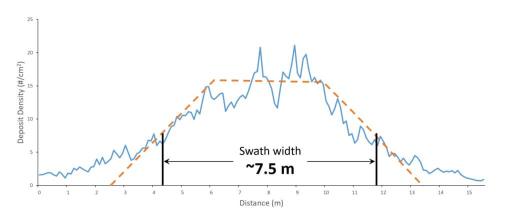
Assuming a trapezoidal-shaped spray swath, the Effective Swath Width (ESW) can be roughly defined as the span between two points that represent 1/2 of the average maximum deposit density. The idea is to create a cumulative pattern that is as uniform as possible when adjacent flights are added (Figure 1).

As with any application system, if we assume that the target rate provides acceptable control, any deviation from the intended target rate along the pattern is either over-dosing (waste), or under-dosing (reduced control). It is therefore imperative that the distributed dose, as received by the intended target, be as uniform as possible.

Materials and Methods

The study was conducted at Ontario’s Simcoe Research Station on September 17, 2024. The site was a flat, sand/loam field with no vegetation present (Figure 2).

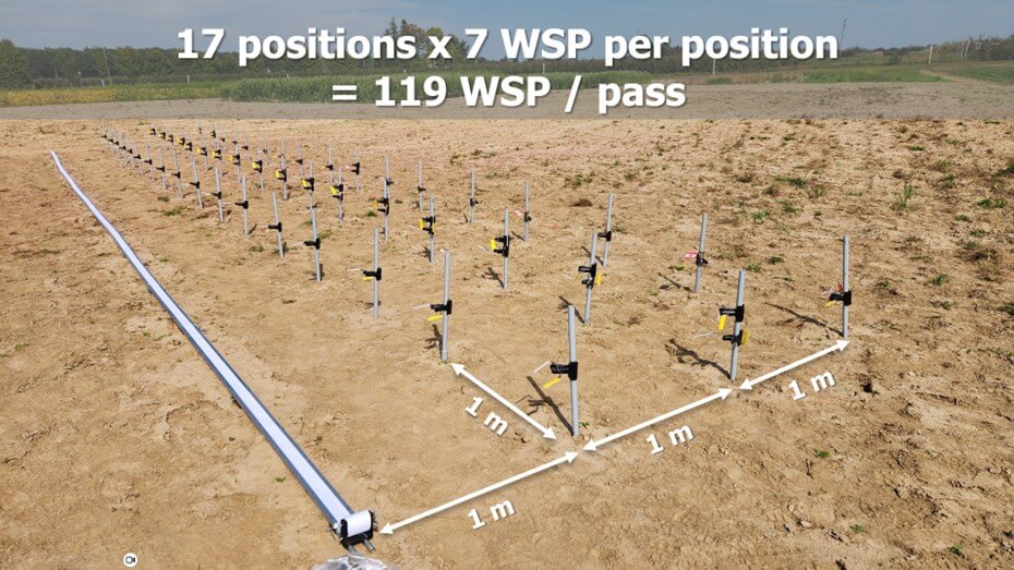
A sampling array was established perpendicular to the forecast prevailing wind direction (150º). The sampling array had 17 discrete sampling locations (0 m to 16 m at 1 m intervals).

Two collector methods were used simultaneously, centered on and perpendicular to the flight path:

1. A flat, horizontal, continuous bond paper strip measuring 7.5 cm wide and 16 m long (secured in a Speed Track™ and analyzed using a Swath Gobbler™, Application Insight, Lansing MI).
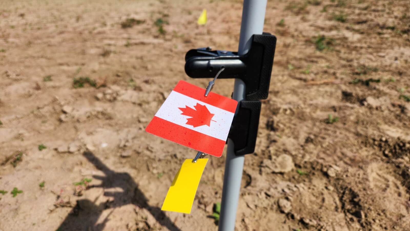
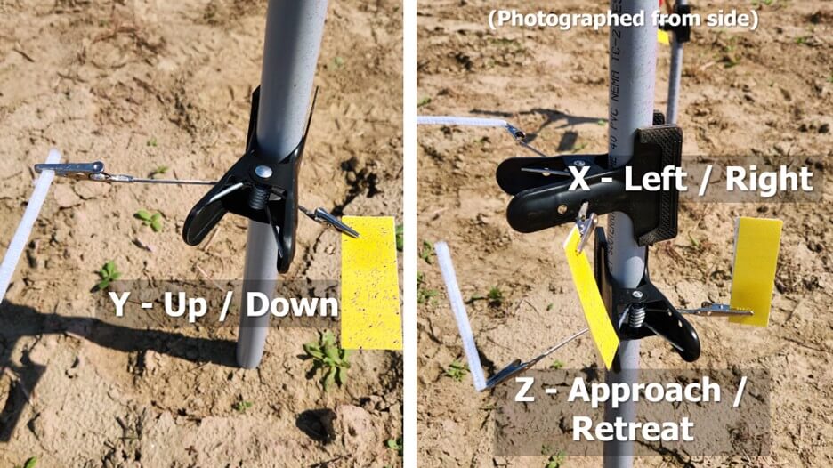
2. Discrete water-sensitive paper (WSP) collectors facing in three directions (x, y, z), each clamped back to back. WSP measured 26 x 76 mm (Spraying Systems, Glendale Heights, IL) and were analyzed using a DropScope™ (SprayX, São Carlos, Brazil).

Sampling height was 30 cm above ground to simulate a fungicide application into a soybean crop. To avoid crowding collectors on each sampler, three parallel sampler rows were established, separated by a 1 m spacing (Figure 3).

The first row contained the WSP and pipe cleaners oriented in the Y direction (WSP facing upward and downward. The second row contained the WSP in the X direction (WSP facing left and right relative to flight direction), as well as Z direction (WSP facing sprayer approach and retreat (Figure 4).

Drone settings

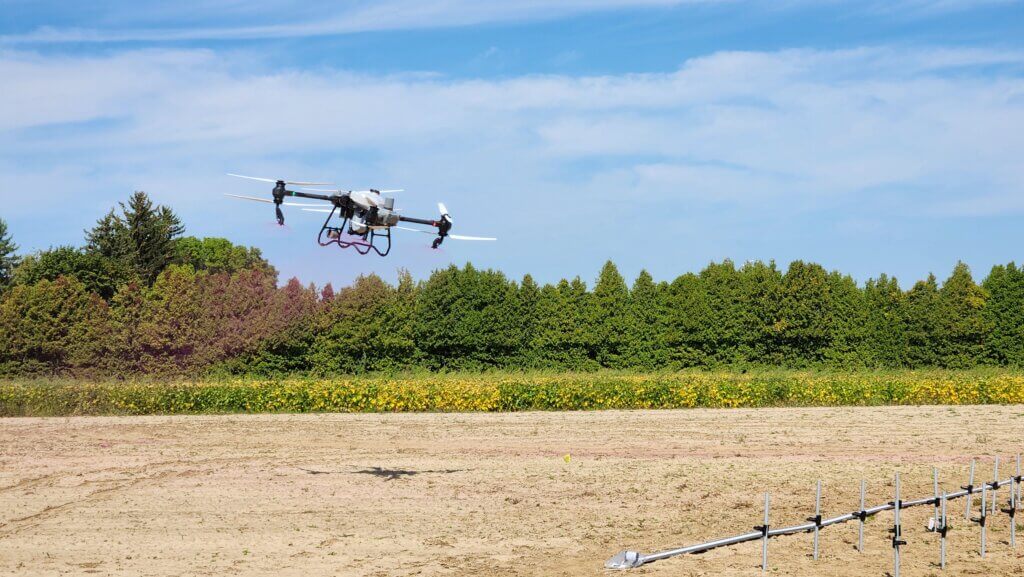
A DJI T50 drone fitted with four rotary atomizers was used to make the spray applications. The flight controller settings were a 250 µm droplet diameter spray over a 7 m swath width, at an altitude of 3 m above ground. Flight speed was either 4 m/s or 8 m/s. Application volume was 30 L/ha. Each flight speed was replicated three times. A total of six passes were made in this trial.

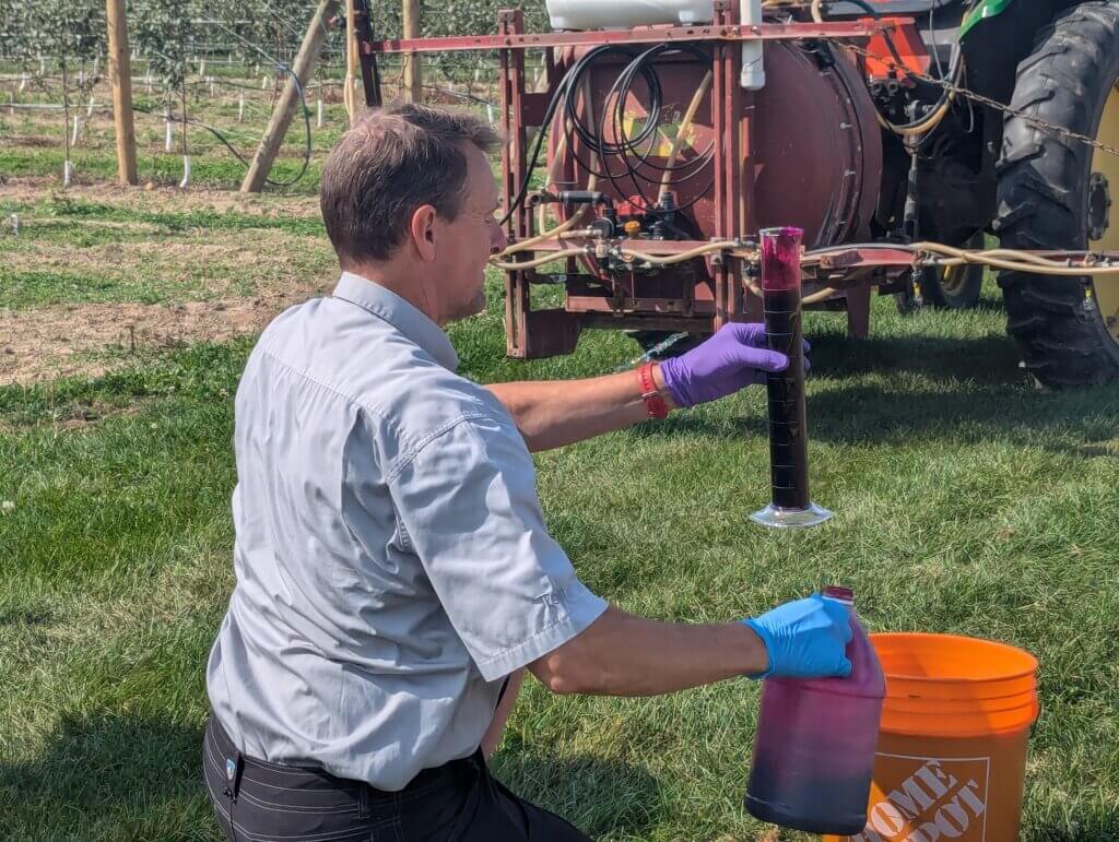
The drone tank (capacity 40 L) contained tap water water with 0.2% v/v of Rhodamine WT 20% liquid (Hoskin Scientific, Burnaby, BC), prepared in a single batch (Figure 5). The level of liquid in the RPAS tank was maintained between 20 L and 30 L throughout the trial to minimize the effect of a changing payload. A volume of spray liquid was sampled prior to each pass to serve as standards for fluorometric analysis.

Trial procedure

Collectors were placed in samplers and the drone was positioned ~75 m downwind of the array to allow it to reach the target flight speed. When wind conditions were deemed appropriate, a signal was given to initiate the flight. Upon pass completion, one minute was allowed to elapse before sampler collection to permit complete deposition and drying.

Labelled WSP were retrieved and placed loosely in paper bags to prevent any residual moisture from ruining the collectors. Bond paper from the Swath Gobbler^™ was marked with treatment information and reeled onto individual spools (one per treatment).

Weather conditions

Both wind speed and direction varied slightly during the study, but it was always possible to run a trial with negligible sidewinds so that the sample array captured the majority of the spray swath. Air temperature was approximately 25 °C. Wind speed was ranged from 6 to 14 km/h during the trial. All spray passes were into a headwind with maximum deviations of -10 to +30°.

Collector analysis

Bond paper digitization

Bond papers (Figure 6) were scanned using a Swath Gobbler^™. The software measured both deposit density and percent coverage at each scanned location, but only deposit density was used in the analysis.

WSP digitzation

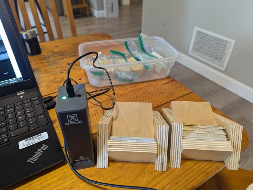
WSP were removed from paper bags, sorted and sequenced into reps. WSP were scanned using a Drop Scope^™ set to “Ground sprayer” and “Syngenta WSP” (Figure 7). The software reported deposit density and percent area coverage, but only deposit density was used in the analysis.

Effective swath width calculation

We used our Excel-based model which assumes a racetrack pattern and sums deposits from adjacent swaths. Swath width was adjusted to minimize over- and under-dosing as well as deposit coefficient of variation (CV), while maximizing swath width.

For the WSP collectors, each of the six orientations were first evaluated separately, and then averaged to simulate a three-dimensional plant structure. Given the similar orientations, the upward-facing WSP and bond paper were used as quality-checks.

Visualizing coverage in three dimensions

In order to understand the direction the spray cloud moved as it imacted the collector array, we declared a dominant side to each of the three cardinal directions, x, y, and z that we captured using the WSP.

• X-axis: Looking in the direction of travel, WSP deposits facing right were subtracted from those facing left.
• Y-axis: WSP facing up minus papers facing down.
• Z-axis: WSP facing the RPAS retreat minus papers facing the advance.

This allowed us to estimate the vectors with which the spray was deposited.

Results and Discussion

Deposits on WSP

We first looked at WSP data to better understand the direction that the droplets flew at the time of impact.

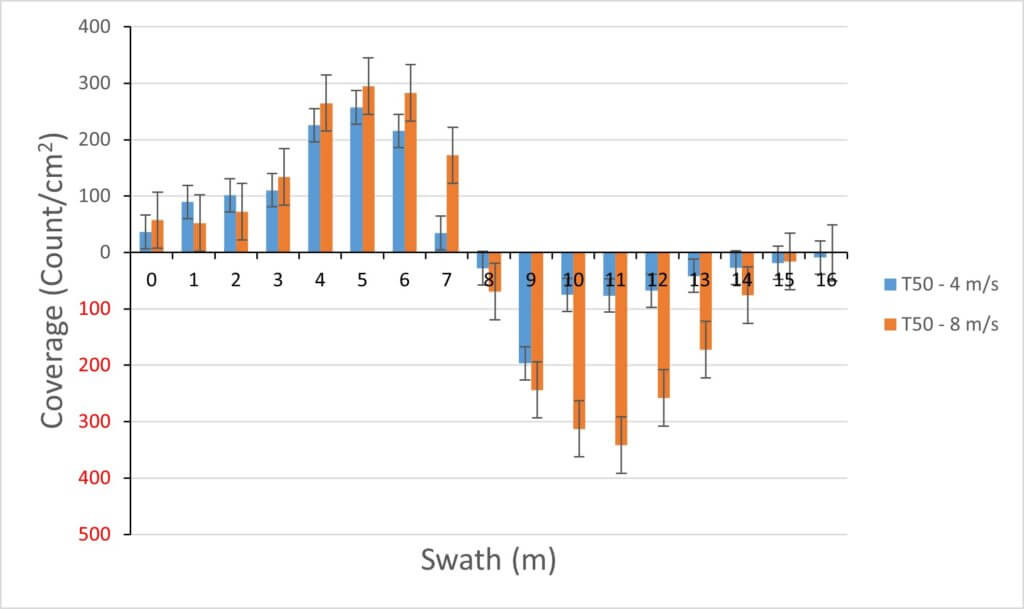
X-axis: Note that the right-facing cards are depicted as being positive, whereas the left-facing cards are depicted as negative.

Only those WSP facing the drone received deposit, with the deposit amount being larger for the faster flight speed (Figure 8). This implies that the spray moved out to either side from the centre of the flight path, carried by a laterally moving downwash.

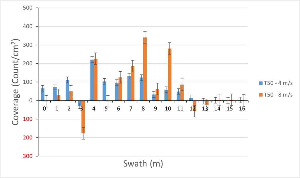
Y-axis: On the whole, deposition on the horozontal collectors was most variable of the three orientations, and resulted in the lowest measured droplet densities (Figure 9). Upward-facing WSP received more of the deposits than the downward-facing WSP. However, at 3 m and 12 m, the majority of deposition appeared on the downward-facing WSP. Underneath the drone rotors, downwash force would prevent re-bound. But at the edge of the rotors, a lower pressure region would permit pressurized air to escape not just laterally but also vertically. Entrained droplets would therefore gain an upward vector, and impact the downward-facing WSP. A slight wind from the right truncated the swath at the 13 m mark. That same wind may have captured any spray from the “bounce” at 3 m to become secondary deposition along the 1 m – 3 m section.

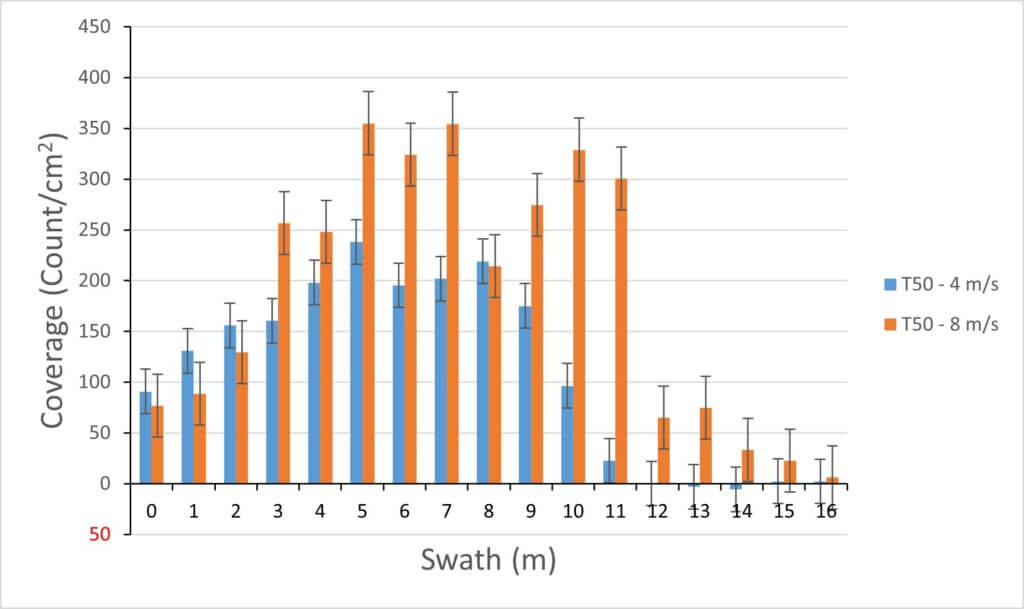
Z-Axis: Only those WSP facing the retreat of the drone received deposits (Figure 10). As previously discussed, this is likely due to the downwash, which is vectored downward and rearward along the flight path according to the drone orientation in flight. These deposits were further reinforced by the prevailing wind direction after the drone had passed.

This deposit pattern is opposite to that of a ground sprayer, where spray tends to deposit on the advance surfaces due to droplet inertia (assuming a low boom height and fast travel speed). A slight shift to the left is apparent in Figure 10, likely due to the headwind’s directional deviation to starboard. Note that the faster flight speed had higher deposit densities. Reasons for this are unclear, as there was no commensurate deficit in droplet numbers at other sampler orientations for the faster speed.

The overall deposit density on the retreat-facing orientation was highest of any single collector orientation. The high deposit density and swath width is likely the result of the prevailing wind direction as well as the additional contribution of the downwash from the forward-tilted RPAS. These two factors helped transport the spray plume backwards for efficient interception by retreat-facing collectors.

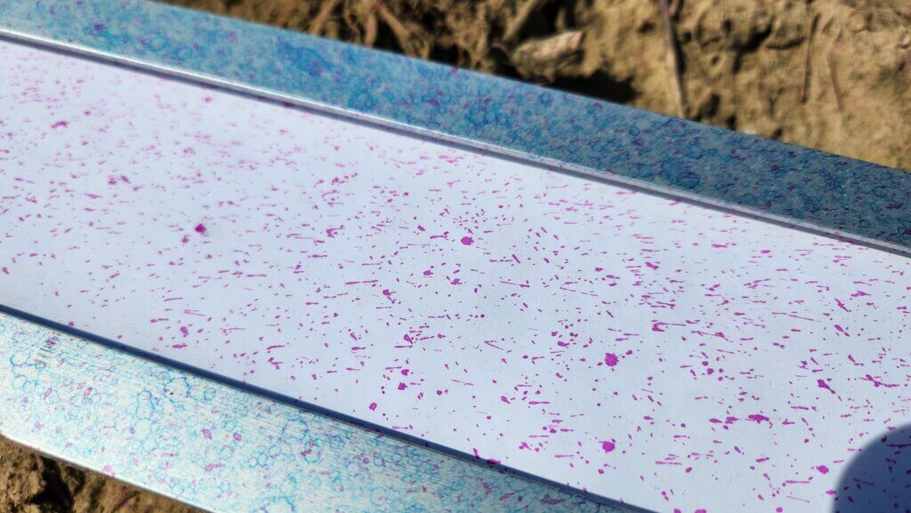
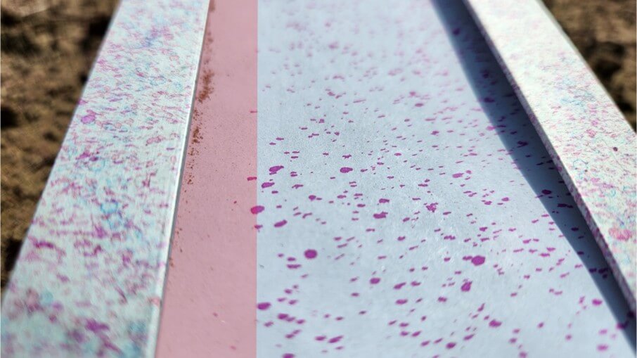
Further evidence of this dynamic was visible when examining the bond paper collector strips. In the lee of the track edge, deposits were scarce, indicating a predominant horizontal trajectory of the droplets (Figure 11).

ESW at 8 m/s flight speed

Only the upward- and retreat-facing WSP surfaces received consistent spray coverage. As a result, only these two orientations were individually used for ESW calculations. However, deposits from all six orientations were averaged for the combined ESW measurement.

Two analysis methods were compared. First, the ESW was calculated for each replicate run seprately, and the resulting ESW were then averaged. Second, the three replicate run deposits were first averaged, and then ESW was calculated from that average.

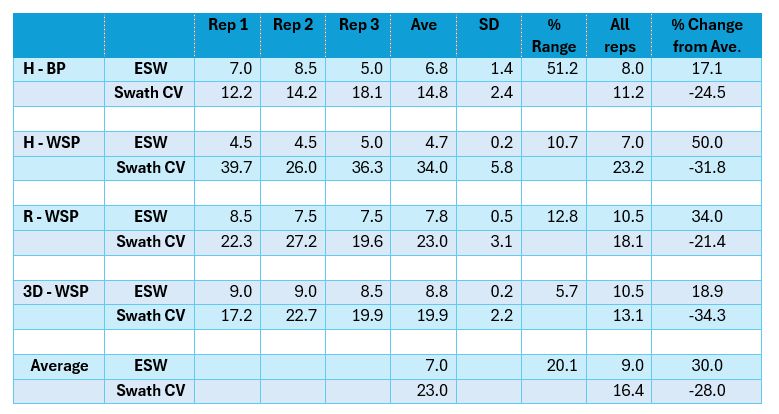
When ESW from the bond paper was calculated for each replicate and then averaged, the ESW was 6.8 ± 1.4 m (Table 1). The resulting average CV of those swaths in a racetrack pattern was 14.8%.

When ESW was calculated from the upward-facing WSP for each replicate, the ESW was 4.7 ± 0.2 m. This was narrower than the bond paper result oriented on the same plane. In addition, the average swath CV was now 34%, significantly higher than that from the bond paper collector.

The retreat-facing WSP resulted in the highest ESW so far, 7.8 ± 0.5 m.

To better simulate a plant’s cumulative deposit, reflecting the pesticide dose received on leaves and stems that might vary in location and orientation, all six orientations were combined for each pass. When ESW was then calculated for each replicate, it was 8.8 ± 0.2 m (CV = 20%).

The range of swath widths onserved within each of the three reps ranged from 6 to 51% of the mean ESW. Differences between replicates could be due to automatic, instantaneous adjustments in the flight path controlled by the drone, or it may be due to changes in environmental conditions in the two hours that elspsed between consecutive replications. It may be instructive to increase the replicate sampling to obtain better estimates of variability within any given treatment.

If reps were pooled before calculating ESW, ESW increased an average of 30% for all sampling methods (Table 1). The CV of multiple swath simulations also decreased an average of 28% with this approach. Pooling prior to analysis is, however, less accurate because it eliminates the variability one might observe between two dicrete locations, which is how product efficacy will be observed in a pest control situation.

ESW at 4 m/s flight speed

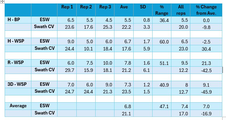
ESW were significantly narrower at the slower flight speed when measured on the bond paper, but of similar widths when merasured using WSP (Table 2). The slower speed had much greater variability among replicate samples as well, ranging from 36 to 60% of the average ESW.

The retreat orientation showed the widest ESW, with the 3D orientations resulting in slightly narrower swaths. At the high speed treatment, the 3D analysis had produced the largest ESW.

Pooling the reps prior to analysis resulted in similar ESW for the bond paper and the upward-facing WSP, whereas the remaining orientations resulted in wider swaths when the reps were pooled.

In general, the swath CVs at the slower flight speed were similar to the fast RPAS speed, averaging in the low to mid 20s. Pooling the reps prior to analysis reduced swath CVs for the retreat orientation and the combined orientations, but not for the upward-facing collectors.

Table 2. Calculated ESW (m) for 4 m/s flight speed based on deposit density (count/cm²). Range (% of mean) calculated for the averages. Change from Average is the % change in the ESW of a pooled sample compared to the averaged ESW from each replicate. H-BP: Horizontal Bond Paper, H-WSP: Horizontal water-sensitive paper, R-WSP: Retreat-facing water-sensitive paper, 3D-WSP: Sum of all six facets of water-sensitive paper.

Comparing speeds

When ESW was calculated for each replicate, the slower flight speed resulted in ESW that were slightly smaller than the faster flight speed on average (6.8 vs 7.0 m). However, when reps were pooled, the slower flight speed resulted in significantly smaller ESW compared to the faster flight speed (7.4 vs 9 m). Pooling the reps prior to analysis also resulted in a lower coefficient of variation.

Generally, there was less variability among replicates for the faster flying speed. Whether this was the result of the speed itself or was an artifact of the specific conditions during which the flights occurred is unclear.

Comparing swath appearance from bond paper and optimal WSP orientations

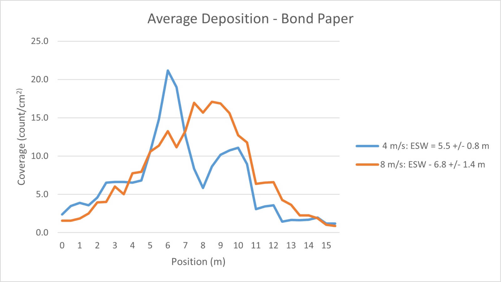
When the ESW from the bond paper was calculated for each replicate and then averaged, the following graph was produced (Figure 12). Note the bi-modal shape produced at the slower flight speed. This corresponds with the position of the atomizers and it’s possible the increased dwell time directed more spray in those positions compared to the faster flight speed, which increased ESW and dispersed the spray more evenly.

This could also be responsible for greater uniformity among the three replicate flights that was observed.

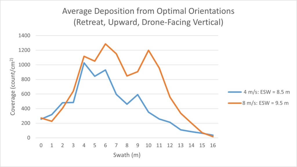
When we averaged coverage from the optimal 3D orientations (X-axis: inward-facing, Y-axis: upward-facing, and Z-axis: retreat-facing) and compared their swaths to the 2D, we are able to capture more droplets and eliminate the bi-modal pattern appearance of the lower speed, reducing CV and increasing the ESW (Figure 13). This may begin to explain why sprays that appear to have low coverage on horizontal collectors can produce better-than expected efficacy.

Vector analysis

The sampler array permitted the generation of spray vectors that showed the inferred direction and intensity of the downwash movement.

To graph vectors for droplet movement at each position along the 16 m swath, we calculated net coverage as previously described (i.e. for each of the x, y, and z sampler oerientations, the deposit density on one side was subtracted from the other). The magnitude of that value represented the relative dominance of that side of the orientation for spray deposition. We assumed that droplets were primarily carried by air movement to their collectors, therefore we inverted the sign on the coverage to express it as wind direction from the from the vantage of the drone. When these data were combined for the X-Y and the X-Z direction, we were able to estimate the origin and strength of the deposit vectors, and thus infer droplet-carrying airflow.

Plotting X by Z meant you are looking down from above (Figure 14). This created vectors that indicate lateral and rearward spray movement.

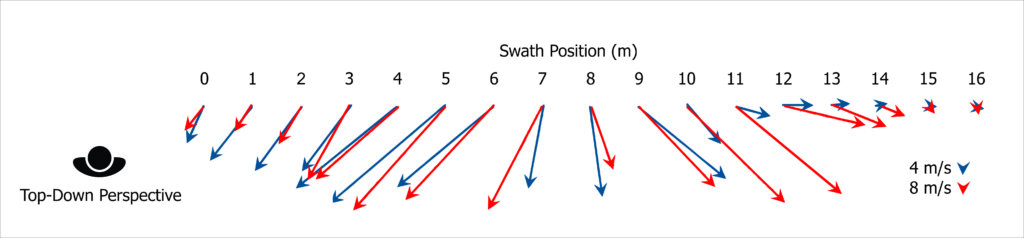
Note that the predominant direction of deposit in the X-Z plane was rearward, in the direction of the wind. The forward-tilt of the RPAS aso directed its downwash towards the rear, adding to the headwind effect. At the edge of the spray swath, the rearward vectors diminished, being solely under the influence of the headwind. The vectors were strongest at the locations corresponding to the RPAS rotors.

Plotting X by Y for each position means looking at the RPAS from ground level as it flies away from you. The resultant vectors indicated a combination of lateral and downward spray movement for the majority of the swath (Figure 15).

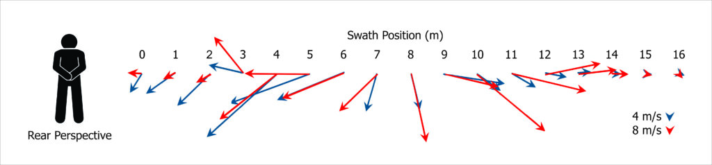
At two locations (3 m and 13 m) the net spray deposition was on the underside of the Y-samplers. This suggested that a special region in the downwash existed, where the high pressure air generated by the rotors dissipated, allowing droplet-laden air to move upwards, essentially re-bounding from the ground. At the same time, droplets moved laterally to escape the same high pressure region.

This region of high turbulence could be where plants in the canopy may see droplets arriving from a large number of directions, contributing to coverage that may not be similarly captured by a single flat collector.

Summary

ESW Measurement Method

There was significant variability in swath width and uniformity among three replicate measurements of the same drone configuration. We observed an average of 34%, and as much as 60%, variation in swath widths within replicate passes of the same speed treatment. Spray deposition cannot be assumed to be repeatable, and understanding deposit variability is likely more important than calculating its average.

Measurement techniques affected the observed swath widths. Generally, horizontal targets resulted in narrower swath width measurements than vertical targets facing into the wind and the direction of drone travel. A composite of various target orientations resulted in the widest and most uniform swath deposits.

Effect of Flight Speed

Faster drone flight speeds resulted in wider measured swath widths in all but one measurment technique. It is possible that the greater concentration of downwash energy at the lower flight prevented more of the droplets from moving laterally prior to impact with a collecting surface.

Measuring Downwash Turbulence

The direction of droplet movement varied with position under the drone. The majority of the droplets had a strong z-vector at deposition. This is the direction of the wind and of the retreating side of the drone. Both wind and backward-tilted downwash of the drone would contribute to this.

As the spray droplets neared the ground, the high air pressure under the drone rotors caused the downwash to move laterally away from the centreline. Droplets entrained in the downwash therefore moved strongly to the left and right of the centreline.

Of the dominant three collector orientations (retreat, lateral, and upwards), the lowest collection was achieved with horizontally oriented targets. Interestingly, at the rotor edge, vortices formed and these moved the droplets upwards, away from the ground. This effect was only observed in a narrow band at he outside edge of the rotors.

These effects were somewhat variable but consistent for all spray passes, and occurred at both travel speeds.

Overall Conclusions

1. A drone’s downwash results in spray droplets moving in many directions which cannot be accurately sampled with a single collector orientation.
2. If only a single plane can be sampled, it should be facing the retreat side of the spray pass.
3. Three-dimensional sampling may be required to better simulate the spray capture of an agricultural canopy.
4. Higher travel speeds resulted in slightly more uniform, wider, and repeatable deposition.
5. The variability of a drone’s deposition, both in ESW and CV, is considerable and remains a barrier for consistent efficacy.
6. Multiple replicate passes, analyzed discretely, are required to understand the variability of the drone’s spray deposit, both in ESC and in CV.

Thanks to Drone Spray Canada and Don Murdoch (University of Guelph) for their cooperation and in kind support of this study.