Crop spraying is one of the most important and highly skilled jobs undertaken on any arable farm, but it is facing increased public scrutiny. This is why it is vital that the kit you use as a means to apply pesticide to crops is in prime working order and is set up correctly to deliver the product safely and accurately to its target. Optimum sprayer set up will help to maximize the efficacy of applied products, reduce spray drift and keep machinery in good condition.
For this best practice guide to sprayer set up, Farmers Weekly teamed up with former Farm Sprayer Operator of the Year Iain Robertson. Mr. Robertson is assistant arable farm manager at David Foot Ltd, a 2,200ha mixed farm south of Dorchester in Dorset, growing wheat, barley, beans, oilseed rape and maize as forage for the farm’s three dairy herds. The machine used for this guide is a Bateman RB26 self-propelled sprayer and while most of these checks and tests are universally applicable to all sprayers, it is also important to refer to the handbook of the manufacturer of your specific machine.
Watch the video tutorial with Mr. Robertson and then see the step-by-step guide below for more detail.
Pre Start Checks
Before firing up the engine, the first thing to do is your pre-start checks – that means checking your machine’s vital fluids like fuel, hydraulic oil, hydrostatic oil, engine oil and coolant levels. If yours is a self-propelled sprayer, chances are you’ll need to get up on to the back of the machine to check some of these.
“While I’m up on the back of the sprayer I also have a quick look in the top of the tank to make sure that it is nice and clean and the tank rinse nozzles have worked properly – cleanliness is next to godliness,” says Mr. Robertson. Next, move on to the tires. Use a pressure gauge to check all tires are at the correct pressure and refer to the manufacturer’s guidelines. If you’ve got a trailed sprayer, don’t forget to check the tractor tire pressures as well.
Aim for tires to be run at the lowest pressure recommended for the load to be carried. This will help with boom height and stability and also helps tires act like a shock absorber to ride out bumps. If using a trailed sprayer, use a spirit level to ensure that the drawbar is level. Mr. Robertson says he tries to work around the machine in a methodical, clockwise manner to ensure that he doesn’t miss anything.
Coming to the pumps, check that they have got enough oil, check that any tool boxes have enough spare parts and any equipment needed and make sure you are carrying a spill kit with absorbent granules and a spade in case the worst happens and there is a spillage. Make sure all parts are lubricated daily and that any grease nipples are cleaned before and after use to avoid them collecting dirt and blocking.
Check all hydraulic hoses, spray lines and air lines for any signs of wear that could result in problems while operating.
It’s best to run the sprayer at a minimum of 5 bar to check for leaks. Also check the spray tank is fixed down securely, all straps and bolts are tight.
Boom checks
Once opened out, check the boom has good movement in the x- and y-axis. All machines are different so check with your manufacturer as to how the boom is set up. Mr Robertson’s Bateman has tie rods and stock bots that can be adjusted to set the boom up to ride well.
Check the tie rod nearest the back of the machine is slightly loose when moving and that the front rod is tight. Next, check for up and down movement by gently pushing the boom down by about 50cm and letting go. The boom should return to the central position without too much bouncing around.
“We want a little bit of movement but not excessive so that you can ride over the bumps as you go along without over- and under-dosing the crop,” says Mr. Robertson. Boom height is one of the most critical factors when spraying and the ideal height is 50cm above the crop. One of the easiest ways to work this out is by using a cable tie that is cut off at the correct length to use a visual aid from the sprayer cab.
Don’t forget to measure from the tip of the nozzle to the crop, not the spray line.
Good sprayer cleanliness is important, so make sure the system is rinsed through at the end of each day with clean water to make sure there’s no residue left in the boom. If your machine’s boom doesn’t have recirculation, remember to take the end caps off occasionally and flush out the whole boom.
Nozzle checks
Check that the nozzles are aligned both vertically and horizontally, according to the NSTS guidelines. Loosen clamps to adjust any nozzles that need realignment.
Check the nozzle output at least twice a year by running the sprayer with clean water at 3 bar pressure. Time the output of each nozzle for 30 seconds. If nozzles have been used previously, it’s best to check their output against that of a new pair. Mr Robertson advises using a measuring cylinder rather than a jug to measure the flow rate as a jug is less accurate “because you get a bigger variation over the wider surface area”.
With an 03 nozzle running for one minute at 3 bar pressure, the output should be 1.2 litres/minute as a rule of thumb but refer to the nozzle manufacturer’s output chart for the expected flow rate. “An easy way to remember this is: at 3 bar your nozzle size multiplied by four will give you your target litres/minute output. It works for all nozzle sizes.” If the output varies more than 4% of the average, or if the spray pattern visually doesn’t look correct, you need to change the nozzle set.
After checking the output, cross-reference this figure with the rate controller – you may need to adjust the flow figures to ensure that the two correlate. If a nozzle becomes blocked while spraying, Mr. Robertson says he will swap it for a new one and then clean it later using a toothbrush or airline. Never blow through a nozzle with your mouth.
Nozzle choice
The choice of nozzle is highly dependent on the sort of job you’re doing. “Timing is crucial but using the right nozzle at the right time will make the job so much easier, cut drift and mean that you’re getting more of the product where you want it to go. If you aim at it you will hit it,” says Mr. Robertson.
His nozzle of choice is an 03 size and he prefers to use the Defy 3D nozzle alternated forwards and backwards across the boom for pre-emergence work and T0 applications as well as the T3 ear spray. “In less than optimum conditions I may prefer to use the Amistar/Guardian Air, a fine induction nozzle. I would use this at T1 and T2 and also in sub-optimum conditions.” This nozzle has a 3-star Local Environmental Risk Assessment for Pesticides (LERAP) rating and is 75% drift reducing.
A water volume of 100 litres/ha is a good rate for spring fungicide application. It provides enough coverage for good disease control and allows maximum efficiency from the sprayer.
Forward speed
The third and final part of reducing spray drift is forward speed. Depending on nozzle size and water volume, aim to travel at 12kph.
Mr Robertson says he finds that this speed gives a good overall output and means you don’t get shadowing or turbulence behind the machine.
Tips and tricks
One of the biggest risk of contamination is at fill up. “A fantastic, cheap trick that I learned through Farm Sprayer Operator of the Year is to take a 200 litre plastic drum and cut it in half to create two drip trays to catch any spillages under the induction hopper and the tank overfill.” This eliminates point source contamination, he says.
“Finally, there’s a plethora of information out there on the internet, loads of good apps to download. The technology is there to help us do the best job possible and make our job as safe as possible.”
We conducted a series of drone deposition studies with three main objectives:
We wanted to:
Measure the swath width of a T50 drone at two flight speeds;
Document the nature of the downwash along the swath width;
Compare different techniques for measuring and analyzing swath widths.
The four swath width measurement methods were:
Horizontal bond paper (H-BP)
Horizontal water-sensitive paper (H-WSP)
Retreat-facing water-sensitive paper (R-WSP)
Three-dimensionally arranged water-sensitive paper (3D-WSP)
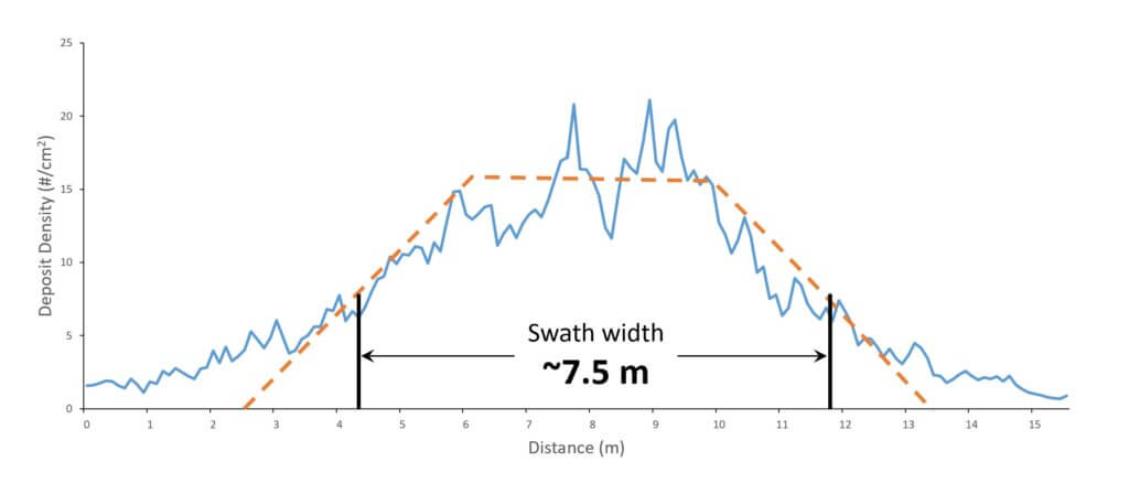
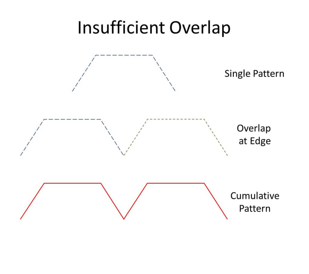
Assuming a trapezoidal-shaped spray swath, the Effective Swath Width (ESW) can be roughly defined as the span between two points that represent 1/2 of the average maximum deposit density. The idea is to create a cumulative pattern that is as uniform as possible when adjacent flights are added (Figure 1).
As with any application system, if we assume that the target rate provides acceptable control, any deviation from the intended target rate along the pattern is either over-dosing (waste), or under-dosing (reduced control). It is therefore imperative that the distributed dose, as received by the intended target, be as uniform as possible.
Figure 1. A spray pattern from DJI Agras T50, as depicted by horizontally oriented bond paper and scanned by Swath Gobbler™. In this case, the effective swath width is estimated from 1/2 the maximum deposit density, spanning approximately 7.5 m.
Materials and Methods
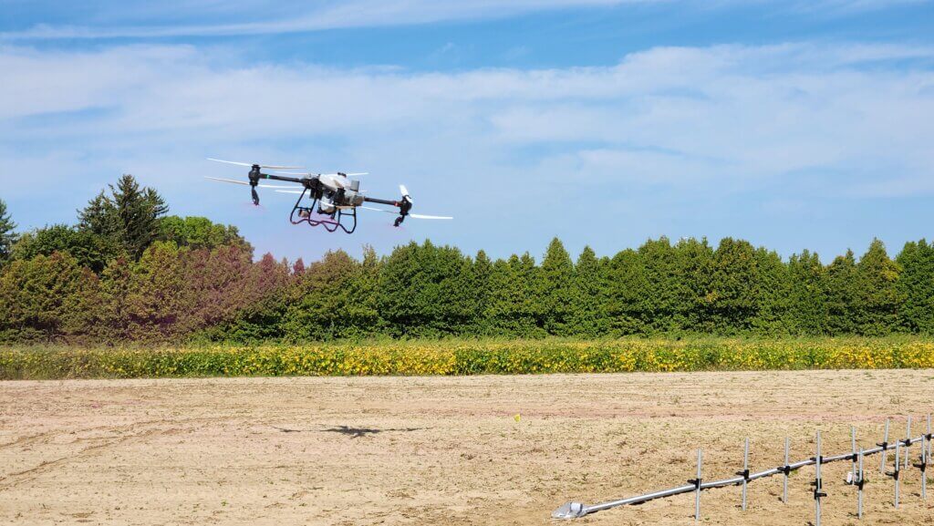
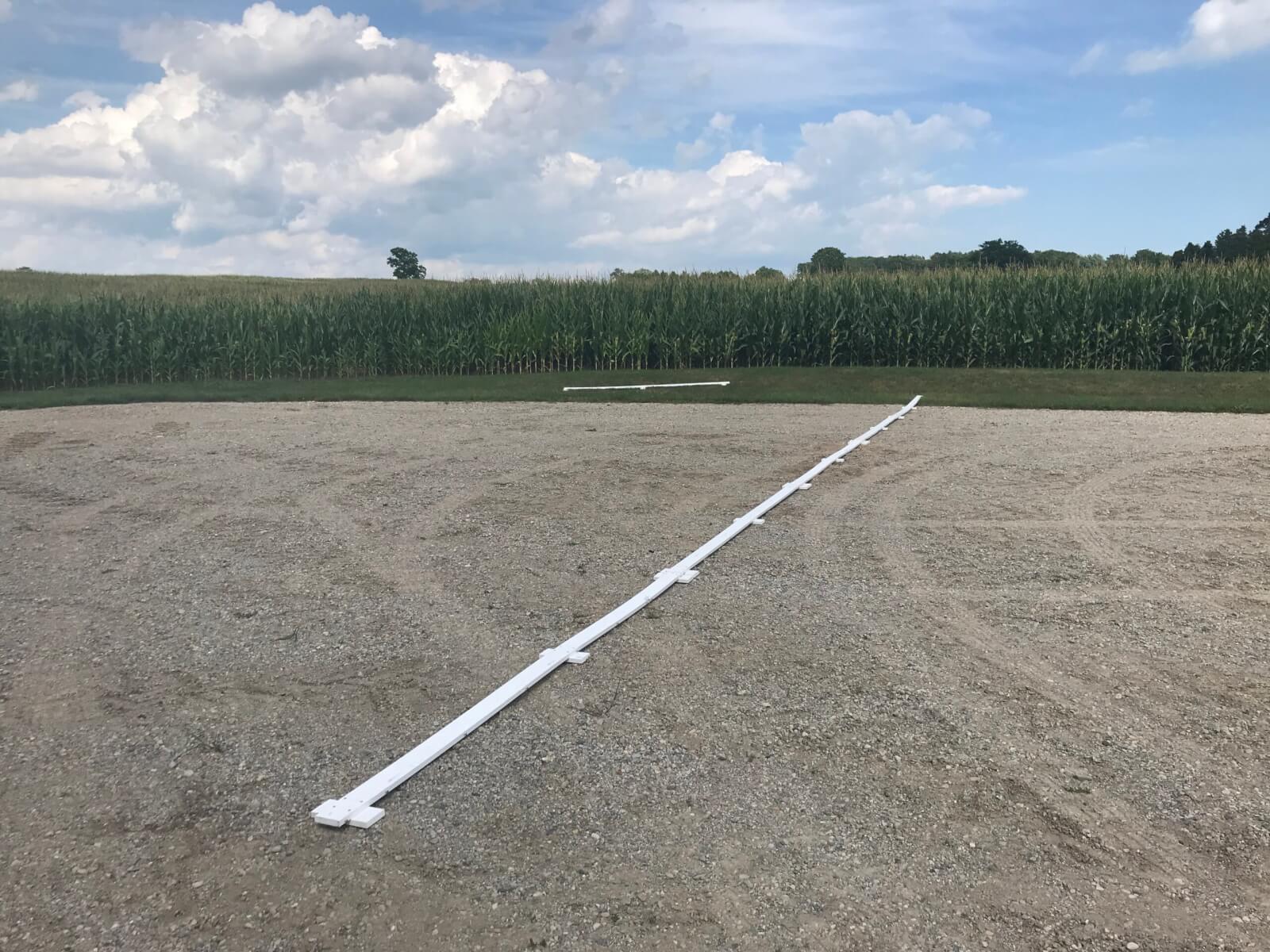
The study was conducted at Ontario’s Simcoe Research Station on September 17, 2024. The site was a flat, sand/loam field with no vegetation present (Figure 2).
Figure 2. Ground conditions at site.
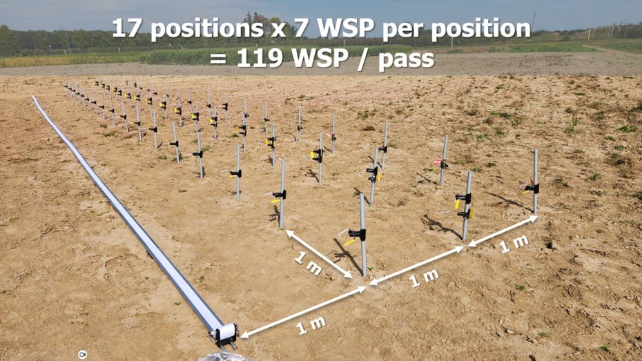
A sampling array was established perpendicular to the forecast prevailing wind direction (150º). The sampling array had 17 discrete sampling locations (0 m to 16 m at 1 m intervals).
Two collector methods were used simultaneously, centered on and perpendicular to the flight path:
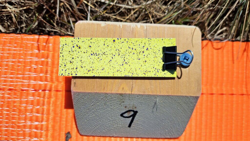
A flat, horizontal, continuous bond paper strip measuring 7.5 cm wide and 16 m long (secured in a Speed Track™ and analyzed using a Swath Gobbler™, Application Insight, Lansing MI).
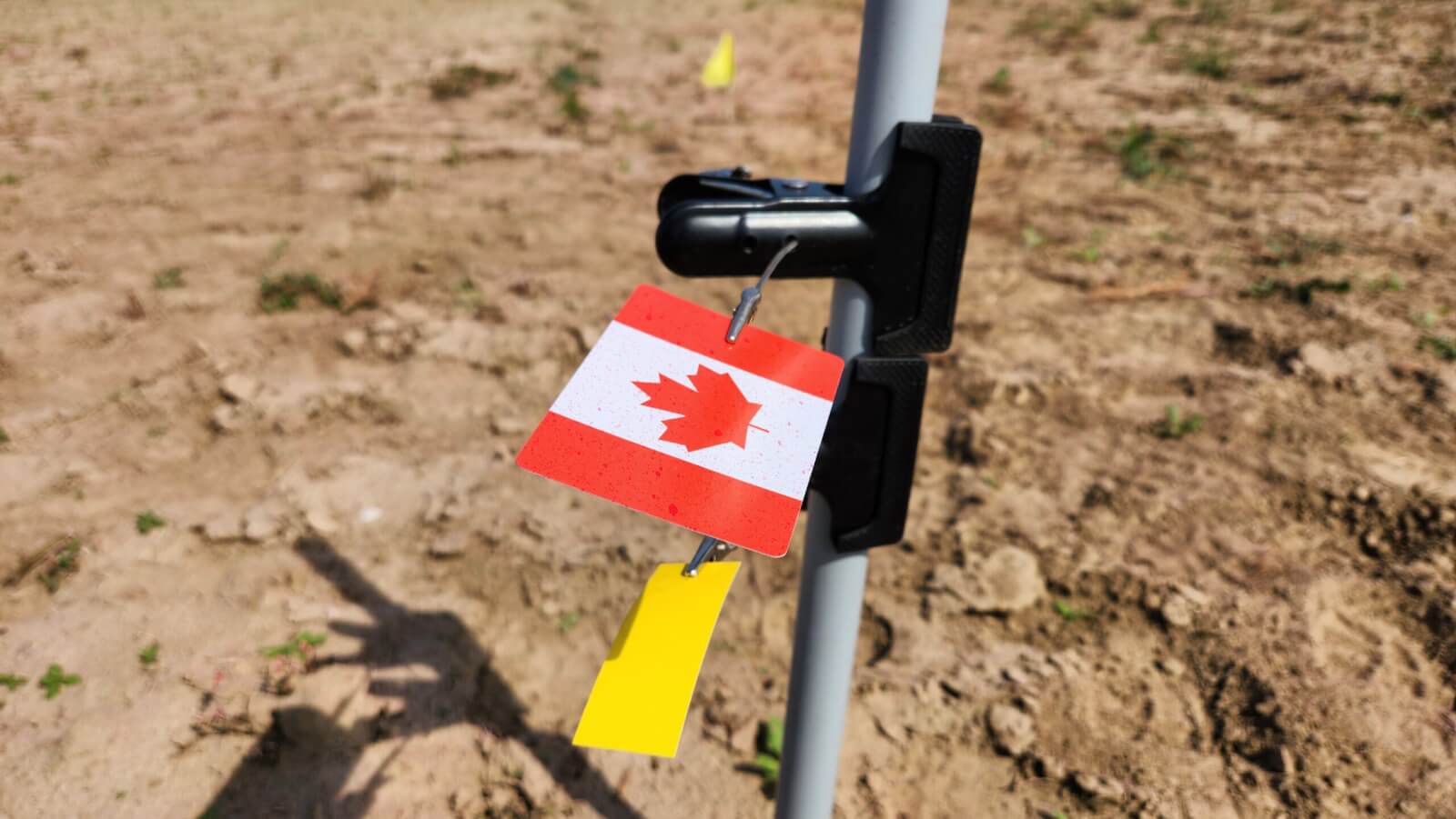
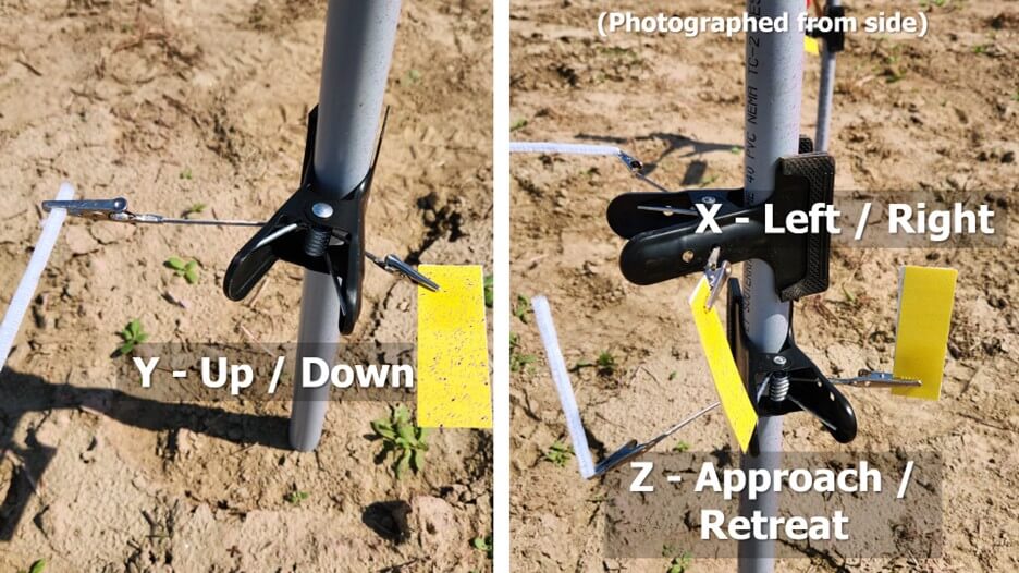
Discrete water-sensitive paper (WSP) collectors facing in three directions (x, y, z), each clamped back to back. WSP measured 26 x 76 mm (Spraying Systems, Glendale Heights, IL) and were analyzed using a DropScope™ (SprayX, São Carlos, Brazil).
Sampling height was 30 cm above ground to simulate a fungicide application into a soybean crop. To avoid crowding collectors on each sampler, three parallel sampler rows were established, separated by a 1 m spacing (Figure 3).
Figure 3. Sampling array and collectors.
The first row contained the WSP oriented in the Y direction (WSP facing upward and downward. The second row contained the WSP in the X direction (WSP facing left and right relative to flight direction), as well as Z direction (WSP facing sprayer approach and retreat (Figure 4).
Figure 4. Examples of discrete sampler design and collector orientation.
Drone settings
A DJI T50 drone fitted with four rotary atomizers was used to make the spray applications. The flight controller settings were a 250 µm droplet diameter spray over a 7 m swath width, at an altitude of 3 m above ground. Flight speed was either 4 m/s or 8 m/s. Application volume was 30 L/ha. Each flight speed was replicated three times. A total of six passes were made in this trial.
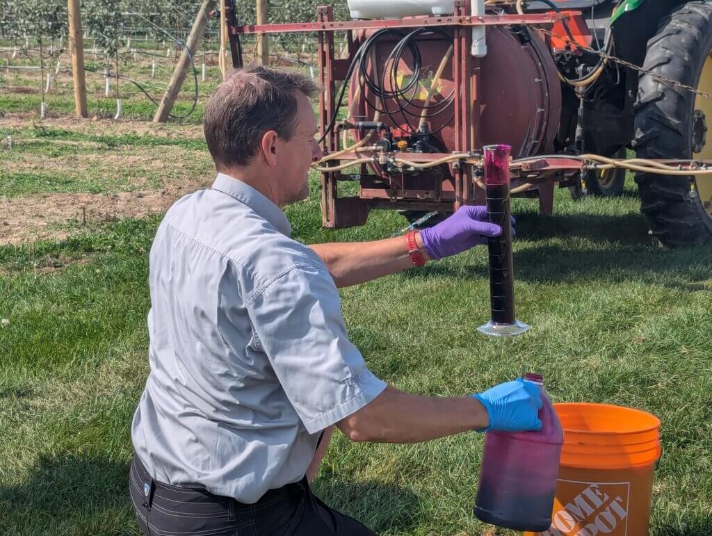
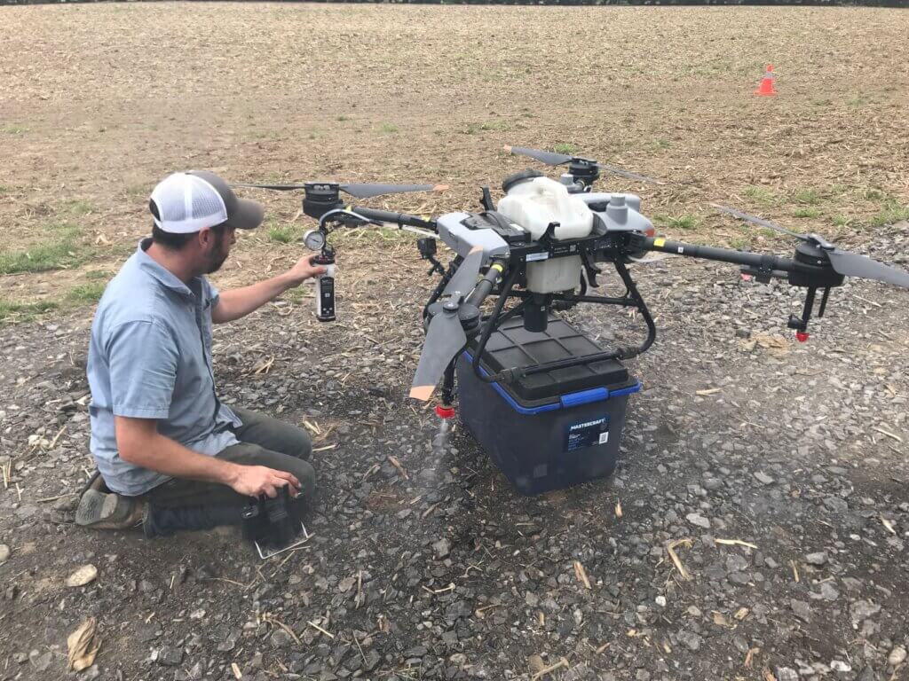
The drone tank (capacity 40 L) contained tap water water with 0.2% v/v of Rhodamine WT 20% liquid (Hoskin Scientific, Burnaby, BC), prepared in a single batch (Figure 5). The level of liquid in the RPAS tank was maintained between 20 L and 30 L throughout the trial to minimize the effect of a changing payload. A volume of spray liquid was sampled prior to each pass to serve as standards for fluorometric analysis.
Figure 5. Preparing the dye solution.
Trial procedure
Collectors were placed in samplers and the drone was positioned ~75 m downwind of the array to allow it to reach the target flight speed. When wind conditions were deemed appropriate, a signal was given to initiate the flight. Upon pass completion, one minute was allowed to elapse before sampler collection to permit complete deposition and drying.
Labelled WSP were retrieved and placed loosely in paper bags to prevent any residual moisture from ruining the collectors. Bond paper from the Swath Gobbler™ was marked with treatment information and reeled onto individual spools (one per treatment).
Weather conditions
Both wind speed and direction varied slightly during the study, but it was always possible to run a trial with negligible sidewinds so that the sample array captured the majority of the spray swath. Air temperature was approximately 25 °C. Wind speed was ranged from 6 to 14 km/h during the trial. All spray passes were into a headwind with maximum deviations of -10 to +30°.
Collector analysis
Bond paper digitization
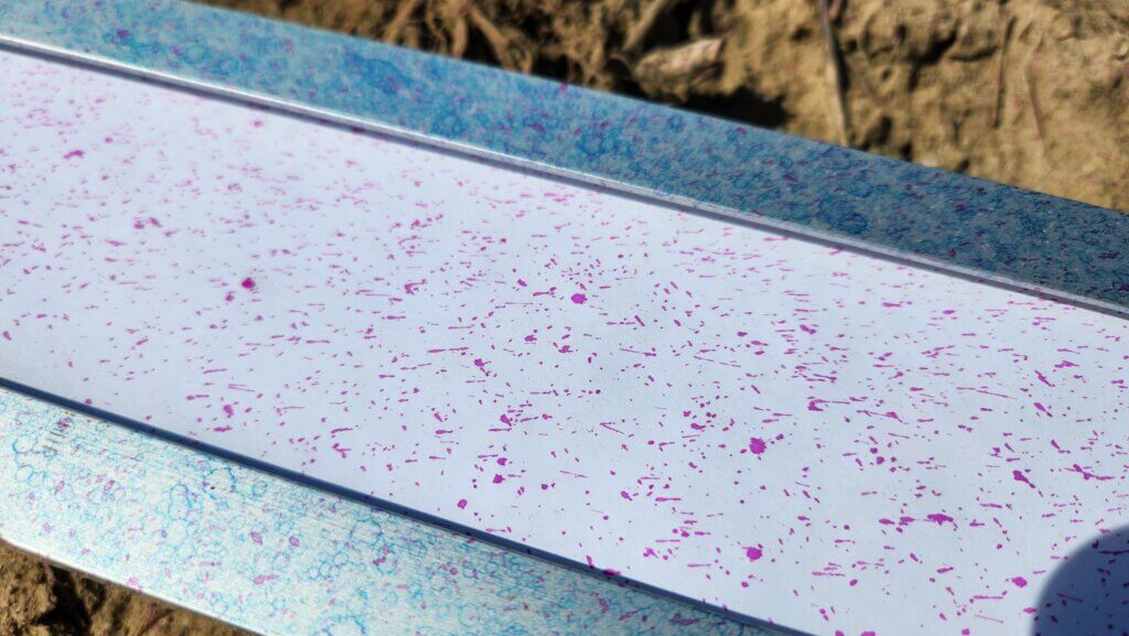
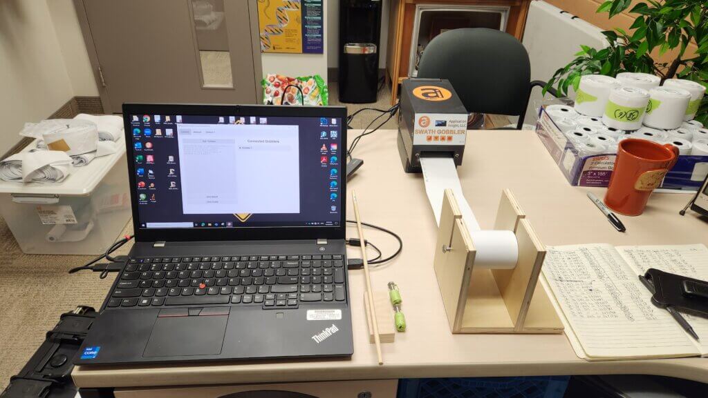
Bond papers (Figure 6) were scanned using a Swath Gobbler™. The software measured both deposit density and percent coverage at each scanned location, but only deposit density was used in the analysis.
Figure 6. Bond paper secured in a Speed Track™ and sprayed with a Rhodamine WT solution.
WSP digitzation
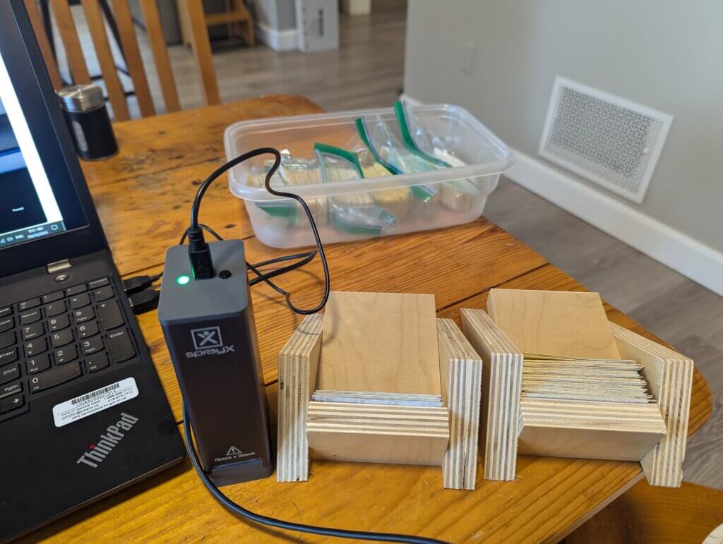
WSP were removed from paper bags, sorted and sequenced into reps. WSP were scanned using a Drop Scope™ set to “Ground sprayer” and “Syngenta WSP” (Figure 7). The software reported deposit density and percent area coverage, but only deposit density was used in the analysis.
Figure 7. In-box, Out-box procedure for scanning WSP using a Drop Scope™.
Effective swath width calculation
We used our Excel-based model which assumes a racetrack pattern and sums deposits from adjacent swaths. Swath width was adjusted to minimize over- and under-dosing as well as deposit coefficient of variation (CV), while maximizing swath width.
For the WSP collectors, each of the six orientations were first evaluated separately, and then averaged to simulate a three-dimensional plant structure. Given the similar orientations, the upward-facing WSP and bond paper were used as quality-checks.
Visualizing coverage in three dimensions
In order to understand the direction the spray cloud moved as it imacted the collector array, we declared a dominant side to each of the three cardinal directions, x, y, and z that we captured using the WSP.
X-axis: Looking in the direction of travel, WSP deposits facing right were subtracted from those facing left.
Y-axis: WSP facing up minus papers facing down.
Z-axis: WSP facing the RPAS retreat minus papers facing the advance.
This allowed us to estimate the vectors with which the spray was deposited.
Results and Discussion
Deposits on WSP
We first looked at WSP data to better understand the direction that the droplets flew at the time of impact.
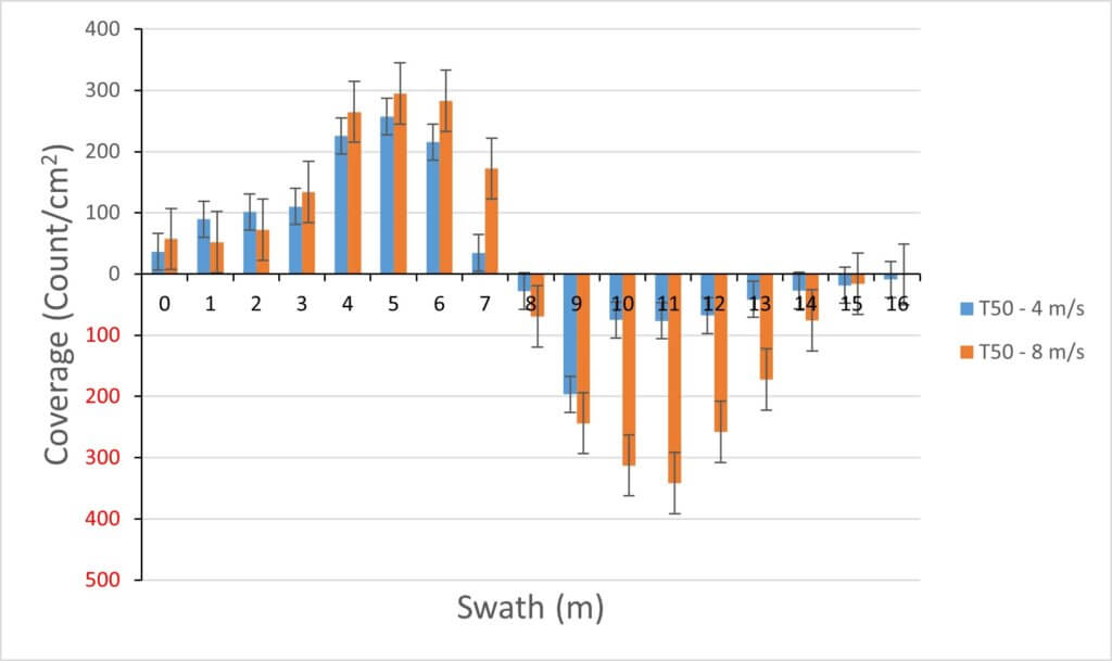
X-axis: Note that the right-facing cards are depicted as being positive, whereas the left-facing cards are depicted as negative.
Only those WSP facing the drone received deposit, with the deposit amount being larger for the faster flight speed (Figure 8). This implies that the spray moved out to either side from the centre of the flight path, carried by a laterally moving downwash.
Figure 8. Coverage on the X-axis, with WSP faces oriented perpendicular to flight path. Note that the drone passed between the 7 and 8 metre marks.
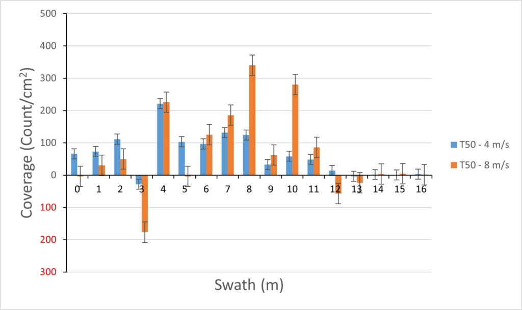
Y-axis: On the whole, deposition on the horozontal collectors was most variable of the three orientations, and resulted in the lowest measured droplet densities (Figure 9). Upward-facing WSP received more of the deposits than the downward-facing WSP. However, at 3 m and 12 m, the majority of deposition appeared on the downward-facing WSP. Underneath the drone rotors, downwash force would prevent re-bound. But at the edge of the rotors, a lower pressure region would permit pressurized air to escape not just laterally but also vertically. Entrained droplets would therefore gain an upward vector, and impact the downward-facing WSP. A slight wind from the right truncated the swath at the 13 m mark. That same wind may have captured any spray from the “bounce” at 3 m to become secondary deposition along the 1 m – 3 m section.
Figure 9. Coverage on the Y-axis, with WSP faces oriented up or down. The drone passed between the 7 and 8 meter marks.
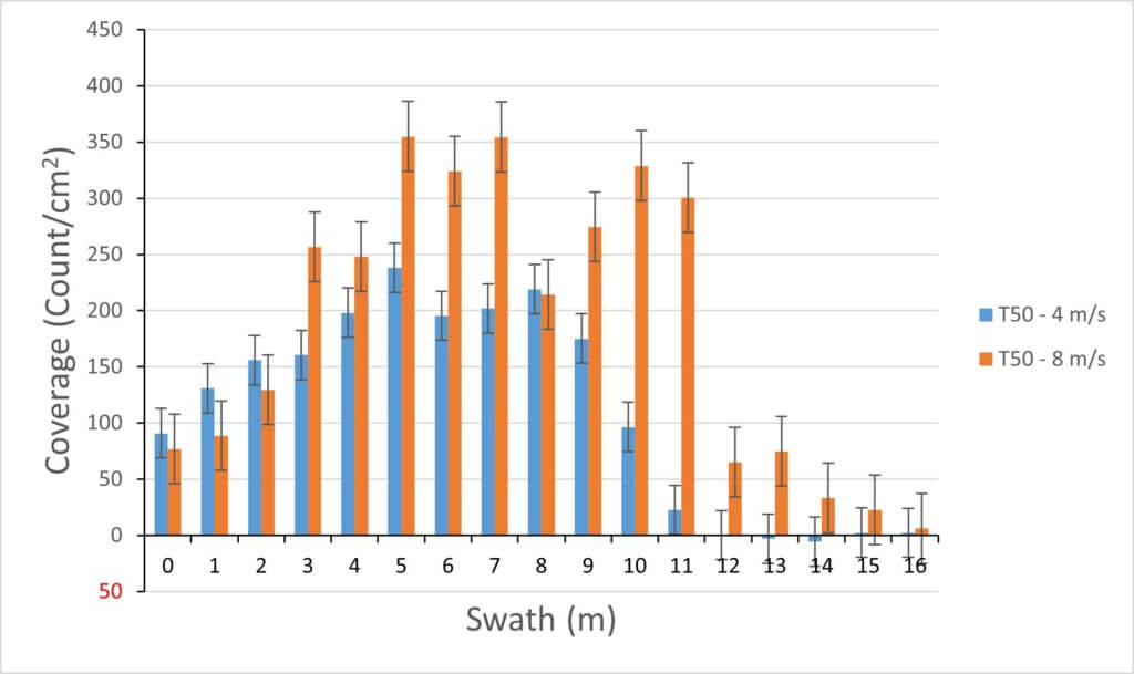
Z-Axis: Only those WSP facing the retreat of the drone received deposits (Figure 10). As previously discussed, this is likely due to the downwash, which is vectored downward and rearward along the flight path according to the drone orientation in flight. These deposits were further reinforced by the prevailing wind direction after the drone had passed.
This deposit pattern is opposite to that of a ground sprayer, where spray tends to deposit on the advance surfaces due to droplet inertia (assuming a low boom height and fast travel speed). A slight shift to the left is apparent in Figure 10, likely due to the headwind’s directional deviation to starboard. Note that the faster flight speed had higher deposit densities. Reasons for this are unclear, as there was no commensurate deficit in droplet numbers at other sampler orientations for the faster speed.
The overall deposit density on the retreat-facing orientation was highest of any single collector orientation. The high deposit density and swath width is likely the result of the prevailing wind direction as well as the additional contribution of the downwash from the forward-tilted RPAS. These two factors helped transport the spray plume backwards for efficient interception by retreat-facing collectors.
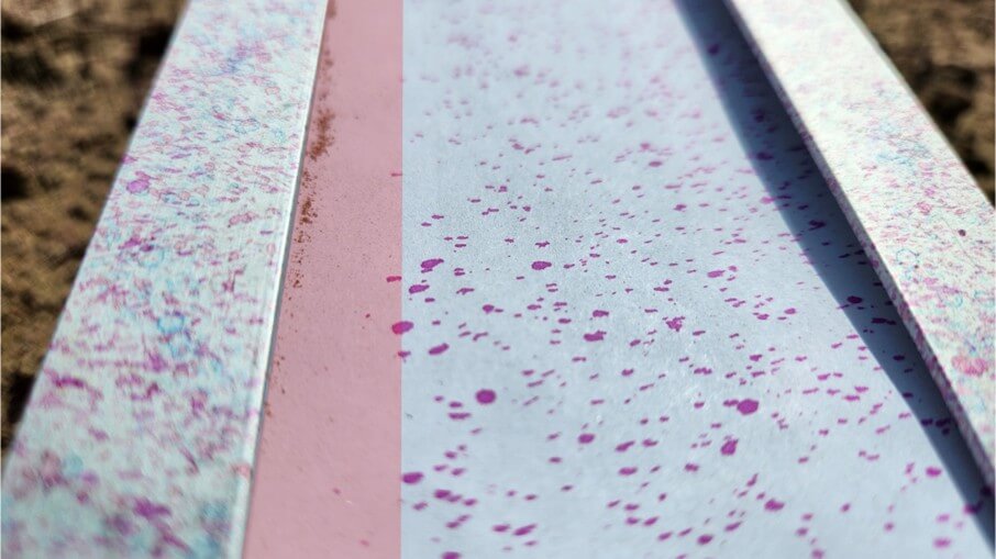
Further evidence of this dynamic was visible when examining the bond paper collector strips. In the lee of the track edge, deposits were scarce, indicating a predominant horizontal trajectory of the droplets (Figure 11).
Figure 10. Coverage on the Z-axis, with WSP faces oriented to face drone advance and retreat. The drone passed between the 7 and 8 meter marks.Figure 11. A shadowed region (highlighted in light red) that sometimes appeared along the retreat-edge of the Speed Track™.
ESW at 8 m/s flight speed
Only the upward- and retreat-facing WSP surfaces received consistent spray coverage. As a result, only these two orientations were individually used for ESW calculations. However, deposits from all six orientations were averaged for the combined ESW measurement.
Two analysis methods were compared. First, the ESW was calculated for each replicate run seprately, and the resulting ESW were then averaged. Second, the three replicate run deposits were first averaged, and then ESW was calculated from that average.
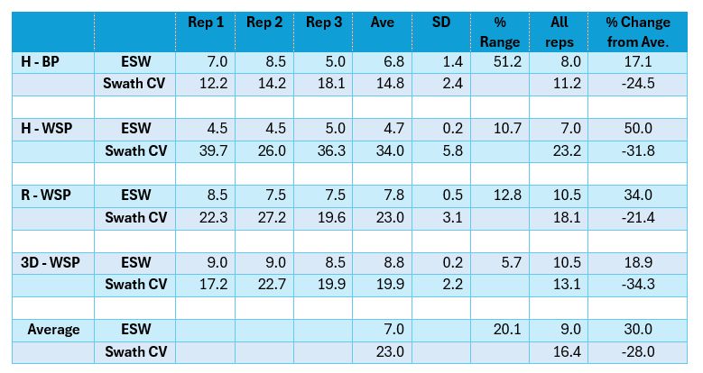
When ESW from the bond paper was calculated for each replicate and then averaged, the ESW was 6.8 ± 1.4 m (Table 1). The resulting average CV of those swaths in a racetrack pattern was 14.8%.
When ESW was calculated from the upward-facing WSP for each replicate, the ESW was 4.7 ± 0.2 m. This was narrower than the bond paper result oriented on the same plane. In addition, the average swath CV was now 34%, significantly higher than that from the bond paper collector.
The retreat-facing WSP resulted in the highest ESW so far, 7.8 ± 0.5 m.
To better simulate a plant’s cumulative deposit, reflecting the pesticide dose received on leaves and stems that might vary in location and orientation, all six orientations were combined for each pass. When ESW was then calculated for each replicate, it was 8.8 ± 0.2 m (CV = 20%).
The range of swath widths onserved within each of the three reps ranged from 6 to 51% of the mean ESW. Differences between replicates could be due to automatic, instantaneous adjustments in the flight path controlled by the drone, or it may be due to changes in environmental conditions in the two hours that elspsed between consecutive replications. It may be instructive to increase the replicate sampling to obtain better estimates of variability within any given treatment.
If reps were pooled before calculating ESW, ESW increased an average of 30% for all sampling methods (Table 1). The CV of multiple swath simulations also decreased an average of 28% with this approach. Pooling prior to analysis is, however, less accurate because it eliminates the variability one might observe between two dicrete locations, which is how product efficacy will be observed in a pest control situation.
Table 1. Calculated ESW (m) and CV (%) for 8 m/s flight speed based on deposit density (count/cm2). Range (% of mean) calculated for the averages. Change from Average is the % change in the ESW of a pooled sample compared to the averaged ESW from each replicate. H-BP: Horizontal Bond Paper, H-WSP: Horizontal water-sensitive paper, R-WSP: Retreat-facing water-sensitive paper, 3D-WSP: Sum of all six facets of water-sensitive paper.
ESW at 4 m/s flight speed
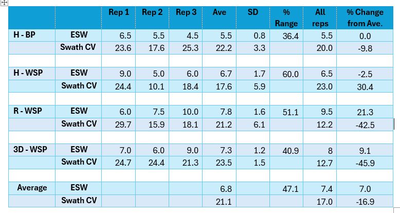
ESW were significantly narrower at the slower flight speed when measured on the bond paper, but of similar widths when measured using WSP (Table 2). The slower speed had much greater variability among replicate samples as well, ranging from 36 to 60% of the average ESW.
The retreat orientation showed the widest ESW, with the 3D orientations resulting in slightly narrower swaths. At the high speed treatment, the 3D analysis had produced the largest ESW.
Pooling the reps prior to analysis resulted in similar ESW for the bond paper and the upward-facing WSP, whereas the remaining orientations resulted in wider swaths when the reps were pooled.
In general, the swath CVs at the slower flight speed were similar to the fast RPAS speed, averaging in the low to mid 20s. Pooling the reps prior to analysis reduced swath CVs for the retreat orientation and the combined orientations, but not for the upward-facing collectors.
Table 2. Calculated ESW (m) for 4 m/s flight speed based on deposit density (count/cm2). Range (% of mean) calculated for the averages. Change from Average is the % change in the ESW of a pooled sample compared to the averaged ESW from each replicate. H-BP: Horizontal Bond Paper, H-WSP: Horizontal water-sensitive paper, R-WSP: Retreat-facing water-sensitive paper, 3D-WSP: Sum of all six facets of water-sensitive paper.
Comparing speeds
When ESW was calculated for each replicate, the slower flight speed resulted in ESW that were slightly smaller than the faster flight speed on average (6.8 vs 7.0 m). However, when reps were pooled, the slower flight speed resulted in significantly smaller ESW compared to the faster flight speed (7.4 vs 9 m). Pooling the reps prior to analysis also resulted in a lower coefficient of variation.
Generally, there was less variability among replicates for the faster flying speed. Whether this was the result of the speed itself or was an artifact of the specific conditions during which the flights occurred is unclear.
Comparing swath appearance from bond paper and optimal WSP orientations
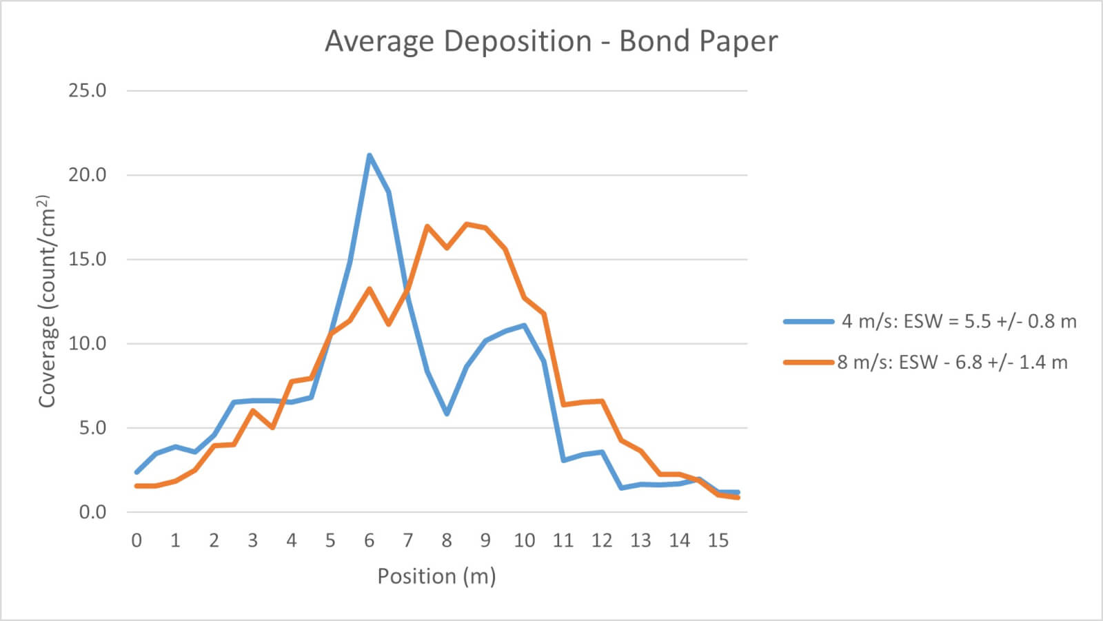
When the ESW from the bond paper was calculated for each replicate and then averaged, the following graph was produced (Figure 12). Note the bi-modal shape produced at the slower flight speed. This corresponds with the position of the atomizers and it’s possible the increased dwell time directed more spray in those positions compared to the faster flight speed, which increased ESW and dispersed the spray more evenly.
This could also be responsible for greater uniformity among the three replicate flights that was observed.
Figure 12. Average of three passes from bond paper at 4 m/s and 8 m/s speed.
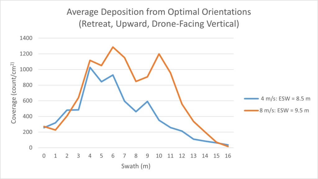
When we averaged coverage from the optimal 3D orientations (X-axis: inward-facing, Y-axis: upward-facing, and Z-axis: retreat-facing) and compared their swaths to the 2D, we are able to capture more droplets and eliminate the bi-modal pattern appearance of the lower speed, reducing CV and increasing the ESW (Figure 13). This may begin to explain why sprays that appear to have low coverage on horizontal collectors can produce better-than expected efficacy.
Figure 13. Average of three passes from optimal-facing WSP samplers at 4 m/s and 8 m/s speed.
Vector analysis
The sampler array permitted the generation of spray vectors that showed the inferred direction and intensity of the downwash movement.
To graph vectors for droplet movement at each position along the 16 m swath, we calculated net coverage as previously described (i.e. for each of the x, y, and z sampler orientations, the deposit density on one side was subtracted from the other). The magnitude of that value represented the relative dominance of that side of the orientation for spray deposition. We assumed that droplets were primarily carried by air movement to their collectors, therefore we inverted the sign on the coverage to express it as wind direction from the from the vantage of the drone. When these data were combined for the X-Y and the X-Z direction, we were able to estimate the origin and strength of the deposit vectors, and thus infer droplet-carrying airflow.
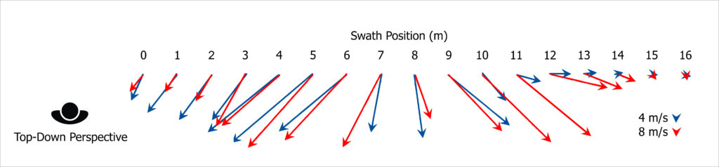
Plotting X by Z meant you are looking down from above (Figure 14). This created vectors that indicate lateral and rearward spray movement.
Figure 14. Plotting X by Z coverage creates vectors that indicate lateral and rearward forces that carry spray droplets released from the drone.
Note that the predominant direction of deposit in the X-Z plane was rearward, in the direction of the wind. The forward-tilt of the RPAS aso directed its downwash towards the rear, adding to the headwind effect. At the edge of the spray swath, the rearward vectors diminished, being solely under the influence of the headwind. The vectors were strongest at the locations corresponding to the RPAS rotors.
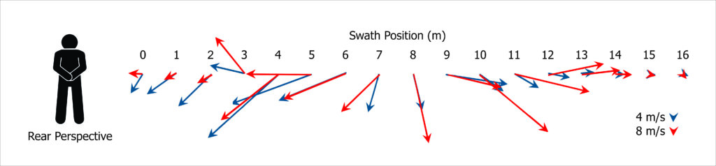
Plotting X by Y for each position means looking at the RPAS from ground level as it flies away from you. The resultant vectors indicated a combination of lateral and downward spray movement for the majority of the swath (Figure 15).
Figure 15. Plotting X by Y coverage creates vectors that indicate lateral and predominantly downward forces.
At two locations (3 m and 13 m) the net spray deposition was on the underside of the Y-samplers. This suggested that a special region in the downwash existed, where the high pressure air generated by the rotors dissipated, allowing droplet-laden air to move upwards, essentially re-bounding from the ground. At the same time, droplets moved laterally to escape the same high pressure region.
This region of high turbulence could be where plants in the canopy may see droplets arriving from a large number of directions, contributing to coverage that may not be similarly captured by a single flat collector.
Summary
ESW Measurement Method
There was significant variability in swath width and uniformity among three replicate measurements of the same drone configuration. We observed an average of 34%, and as much as 60%, variation in swath widths within replicate passes of the same speed treatment. Spray deposition cannot be assumed to be repeatable, and understanding deposit variability is likely more important than calculating its average.
Measurement techniques affected the observed swath widths. Generally, horizontal targets resulted in narrower swath width measurements than vertical targets facing into the wind and the direction of drone travel. A composite of various target orientations resulted in the widest and most uniform swath deposits.
Effect of Flight Speed
Faster drone flight speeds resulted in wider measured swath widths in all but one measurement technique. It is possible that the greater concentration of downwash energy at the lower flight speed prevented more of the droplets from moving laterally prior to impact with a collecting surface.
Measuring Downwash Turbulence
The direction of droplet movement varied with position under the drone. The majority of the droplets had a strong z-vector at deposition. This is the direction of the wind and of the retreating side of the drone. Both wind and backward-tilted downwash of the drone would contribute to this.
As the spray droplets neared the ground, the high air pressure under the drone rotors caused the downwash to move laterally away from the centreline. Droplets entrained in the downwash therefore moved strongly to the left and right of the centreline.
Of the dominant three collector orientations (retreat, lateral, and upwards), the lowest collection was achieved with horizontally oriented targets. Interestingly, at the rotor edge, vortices formed and these moved the droplets upwards, away from the ground. This effect was only observed in a narrow band at he outside edge of the rotors.
These effects were somewhat variable but consistent for all spray passes, and occurred at both travel speeds.
Overall Conclusions
A drone’s downwash results in spray droplets moving in many directions which cannot be accurately sampled with a single collector orientation.
If only a single plane can be sampled, it should be facing the retreat side of the spray pass.
Three-dimensional sampling may be required to better simulate the spray capture of an agricultural canopy.
Higher travel speeds resulted in slightly more uniform, wider, and repeatable deposition.
The variability of a drone’s deposition, both in ESW and CV, is considerable and remains a barrier for consistent efficacy.
Multiple replicate passes, analyzed discretely, are required to understand the variability of the drone’s spray deposit, both in ESW and in CV.
Author’s Note: Newer 3D deposition studies have revealed additional information that should be considered. Read more here
Thanks to Drone Spray Canada and Don Murdoch (University of Guelph) for their cooperation and in kind support of this study.
Alternate Row (aka Alternate Row Middle [ARM]) spraying is an application method where the air-assist sprayer does not pass down every alley during an application. The sprayer operator is relying on the spray to pass through one or more rows and provide acceptable coverage to the entire canopy (or canopies) on a single pass.
Some state agencies promote this spraying strategy to various degrees, and many sprayer operators (whether they admit it or not) have used this method of spraying. I have advised it myself for very young and/or very sparse vineyard and orchard plantings, but never without confirming coverage. When I tell operators that I have serious reservations about alternate row spraying, they defend it. Here are the most common justifications I’ve heard over the years, and my response:
Justification
Reply
“I do not have enough spray capacity to spray every row when time is short.”
You need more sprayer capacity. Get another sprayer so you can get spray on in time or invest in a multi-row sprayer is possible.
“ARM spraying saves money and reduces environmental impact because I use less pesticide.”
Technically, if you travel every second row with a sprayer calibrated to travel every row, you have indiscriminately reduced your carrier and chemical inputs by half (or more). Without close monitoring you may compromise your efficacy.
“I only perform ARM spraying early in the season when canopies are empty, or only on young plantings.”
I grudgingly grant this one as long as coverage is closely monitored. I’ve prescribed it myself in young or sparse plantings where I couldn’t get the sprayer output low enough to prevent drenching the targets.
“The spray plume in the alley beyond the target row must mean the spray is providing adequate coverage. More is better!”
If the spray is blowing through the canopy, it isn’t landing in the canopy. Further, if the air speed/volume is too high, droplets can ‘slipstream’ past the target without impinging on them. I’ve removed water-sensitive paper from canopies with barely any spray on them despite the plume in the downwind alleys. It looks like a magic trick, albeit an unhappy one.
“Uncooperative weather doesn’t always leave me enough time to spray the entire crop, and it is the lesser of two evils to spray alternate rows than not at all. I’ll make sure I come back to spray the other rows later.”
Choosing to do half a job requires an understanding of the products’ mode of action. If you are spraying an insect at a particular stage of development, there’s no “coming back later” to get that generation – if you missed, your window has closed. If it’s a protective fungicide that offers no kick-back, then once the disease has infected tissue, the damage is done. Get the spray on as best you can, but if it washes away before it has a chance to dry sufficiently, be prepared to reapply at the earliest opportunity as long as the label allows it.
“ARM has always worked in the past.”
Would you mind picking my lotto numbers for me? You’re a very lucky person!
My reservations about ARM spraying come from published research and personal experience that show that coverage is almost always compromised when spraying from one side of a canopy. The spray must pass through the canopy to reach the far side, and the canopy filters droplets from the air as it passes through. This reduces the number of droplets available to cover the far side. In addition, high velocity spray will create “shadows” where any targets on the immediate far side of a leaf or branch become shielded and receive little if any coverage. Further still, fine droplets slow quickly as they leave the nozzle and take a long time to settle. As the entraining air slows and becomes erratic, the droplets float and change course, making their behaviour hard to predict.
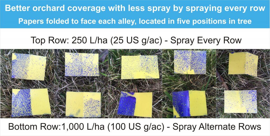
The cumulative impact can be seen in this infographic I built in 2016. The orchardist was a dyed-in-the-wool ARM applicator and he was resistant to driving every row because it took so much time. I wanted to show that he could claw back some of the lost time by spraying less pesticide every row versus his current volume every second row. He would need fewer refills, and save a LOT of unnecessary pesticide. The water sensitive paper does the talking, and while I’d like to think I’ve convinced him, I’ll bet he’s still out there dicing with fate.
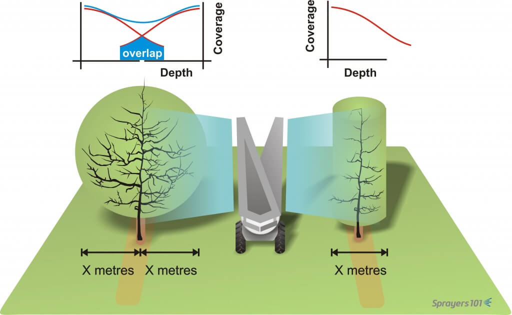
A very popular argument in favour of ARM spraying comes from orchardists that are shifting from semi dwarf to high-density plantings. They ask “How it is different to spray a four foot diameter tree from one side compared to an eight foot diameter tree from both sides”?
Well, we know coverage is reduced as a factor of distance. Spraying from one side gives a single opportunity to cover the middle and far side of a canopy, whereas spraying from both sides provides an opportunity for an overlap in coverage. Essentially, the centre of a canopy receives the cumulative benefit of two sprays. Coverage is therefore always improved when spraying from both sides, period.
Spraying from one side gives a single opportunity to cover the far side of a canopy. However, spraying from both sides provides an opportunity for an overlap in coverage. In other words, the centre of a canopy receives less spray than the outside, but is essentially sprayed twice resulting in a compounding effect.
Why, then, do some sprayer operators claim that alternate row applications work? Because sometimes, they do! Just because coverage is reduced doesn’t mean it isn’t sufficient to protect the crop. It simply means that the potential for poor coverage and reduced dose is dramatically increased by alternate row applications. A sprayer operator might perform alternate applications successfully for years before conditions conspire to defeat the application: unfavourable wind, poor timing, increased pest pressure, poor pruning practices, excessive ground speed, high temperatures, low humidity, insufficient spray volume, and several other factors might occur simultaneously and reduce coverage below a minimal threshold for control. This confluence of bad luck may not happen the first year, or the second, but eventually…
Product failure isn’t the only concern. Repeated reduced dosages may play a role in developing resistance. In those situations where the operator recognizes insufficient coverage, they may have to spray more often to compensate, negating any savings in time or product. Reduced dosage is a common error when a sprayer operator elects to use ARM.
If you still aren’t convinced, at least perform alternate row spraying the “right” way. Here are three situations that I’ve heard operators refer to as alternate row spraying. Situation 1 is most common, but to my mind only Situation 2 would be considered acceptable. Even then, confirming coverage is a must.
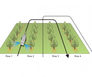
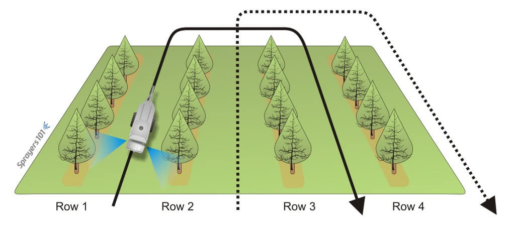
Situation 1:
The sprayer has a typical calibration for spraying every row, but only drives alternate rows. The first application (solid line) covers different rows from the second application (broken line). The operator will claim to spray more frequently, but generally does not perform the second application unless there is high pest pressure. The result is half-a-dose per hectare per application.
The sprayer has a typical calibration for spraying every row, but only drives alternate rows. The first application (solid line) covers different rows from the second application (broken line). The operator will claim to spray more frequently, but generally does not perform the second application unless there is high pest pressure. The result is half-a-dose per hectare per application.
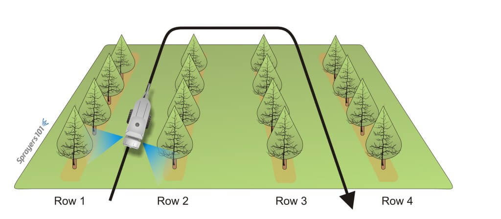
Situation 2:
The sprayer is calibrated for double output compared to a typical every-row situation, and the operator drives alternate rows. The result is that the hectare gets the whole dose per application, but coverage is always inconsistent.
The sprayer is calibrated for double output compared to a typical every-row situation, and the operator drives alternate rows. The result is that the hectare gets the whole dose per application, but coverage is always inconsistent.
Situation 3:
Since the sprayer will only drive alternate rows, the operator mistakenly sets the sprayer to emit half the output compared to a typical every-row situation. The first application (solid line) covers different rows from the second application (broken line). The result is a quarter-dose per application, and if the operator chooses to spray a second time, the hectare will only ever get half-a-dose. Yes, this happens.
The sprayer has a typical calibration for spraying every row, but only drives alternate rows. The first application (solid line) covers different rows from the second application (broken line). The operator will claim to spray more frequently, but generally does not perform the second application unless there is high pest pressure. The result is half-a-dose per hectare per application.
So, my final word on alternate row applications is that they should be performed with extreme caution. I’ve used them myself in early season applications in new plantings, but never without confirming coverage with water-sensitive paper, and never in conditions that might further compromise coverage to the point that the application does not give control.
Caveat Emptor!
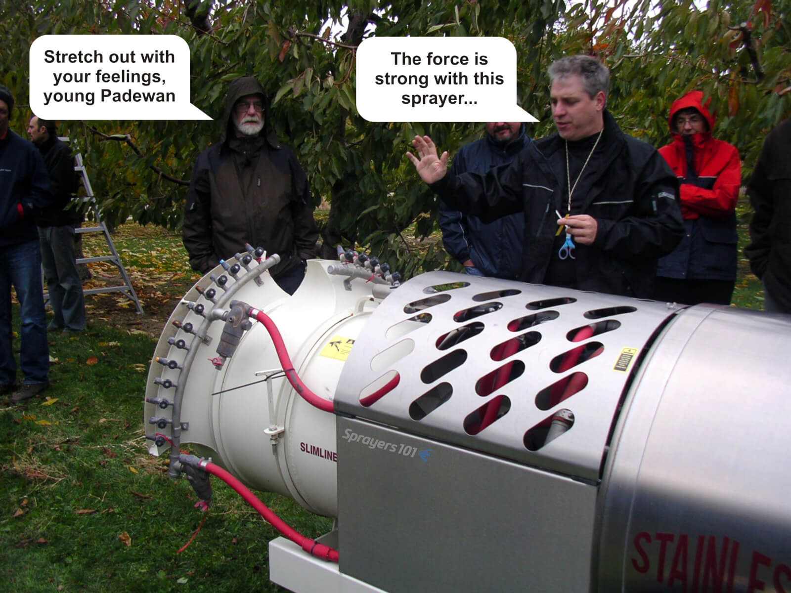
Well, I thought it was funny. My apologies to J. Luymes from British Columbia (pictured) and Obi Wan Kenobi (not pictured… or is he?)
In April 2025 we visited Cedarline Greenhouses to assess their spraying methods. Our hosts invited us to examine their practices and then graciously agreed to let us share the process (and the results) so others could learn from the experience. Every greenhouse is different, but with a little imagination the process we used should translate to most operations. I want to be clear that this operation was already doing a good job before we showed up. It’s just easier for someone from the outside to scrutinize and find little things that might need tweaking. Let’s go through the steps we took that day.
1. Measure the crop canopy and the planting architecture
The objective of any spray application is to achieve sufficient coverage of the target with as little waste as possible. Achieving this goal means understanding the interaction between the sprayer, the spray droplets, and the crop canopy.
Start by measuring the the planting architecture. These values allow us to calculate application rates and to calibrate the sprayer. Cedarline is a 16-acre pepper operation. The crops are strung vertically in double rows for a total canopy depth of about 1 m, leaving roughly 0.5 m clearance in the alleys. Spraying takes place while the crop is between 1.5 and 3.5 m high. Each row is 102 m long.
2. Consider the target from the droplet’s perspective
Stand between the rows and face the canopy. Where is your spray target relative to the nozzle? Is it in line-of-sight, or are there parts of the canopy in the way? In this case, our primary targets are sucking insects found predominately on the under-side (abaxial) surface of the leaves, and not the waxier, above-side (adaxial) faces.
As we look through the double row, we see the adaxial sides face out towards the alleys, and the abaxial sides face the canopy interior. Bad luck. But, as we peer through that first row to the second row, we can see the abaxial sides of those leaves. So, perhaps enough of the spray can penetrate past the first row to deposit on the abaxial surfaces of the far row? This is a tricky plan because of the physics of droplet behaviour.
We know that coarser droplets move ballistically (e.g. like cannon balls), so perhaps they could span the distance from the first row to the next. But they are prone to bouncing and running off surfaces, which means they’d likely drench the waxy adaxial side of the first row before any get to the abaxial side of the far row… and those that do might not stick to the target.
On the other hand, finer droplets are less prone to run off, so they’re much better at sticking to hard-to-wet surfaces like peppers and waxy leaves. Additionally, thanks to the cubic relationship between droplet size and volume, the smaller the average droplet size, the more droplets we have working for us. However, finer droplets don’t have a lot of mass, so they move erratically, and they are prone to evaporation. Maybe they won’t reach deeply enough into the row.
Fortunately, greenhouses are humid places, so finer droplets don’t evaporate quickly. Plus, greenhouses tend to spray at relatively high pressure (200 psi or more), which imparts momentum to finer droplets. Also, when enough tiny particles move in a single direction, they create air currents – essentially a light wind. This side-effect is sometimes enough to move leaves, creating holes in the canopy and exposing the abaxial sides of leaves as they twist. So, there’s hope. Now let’s look at the sprayer.
3. Examine the sprayer and the nozzles
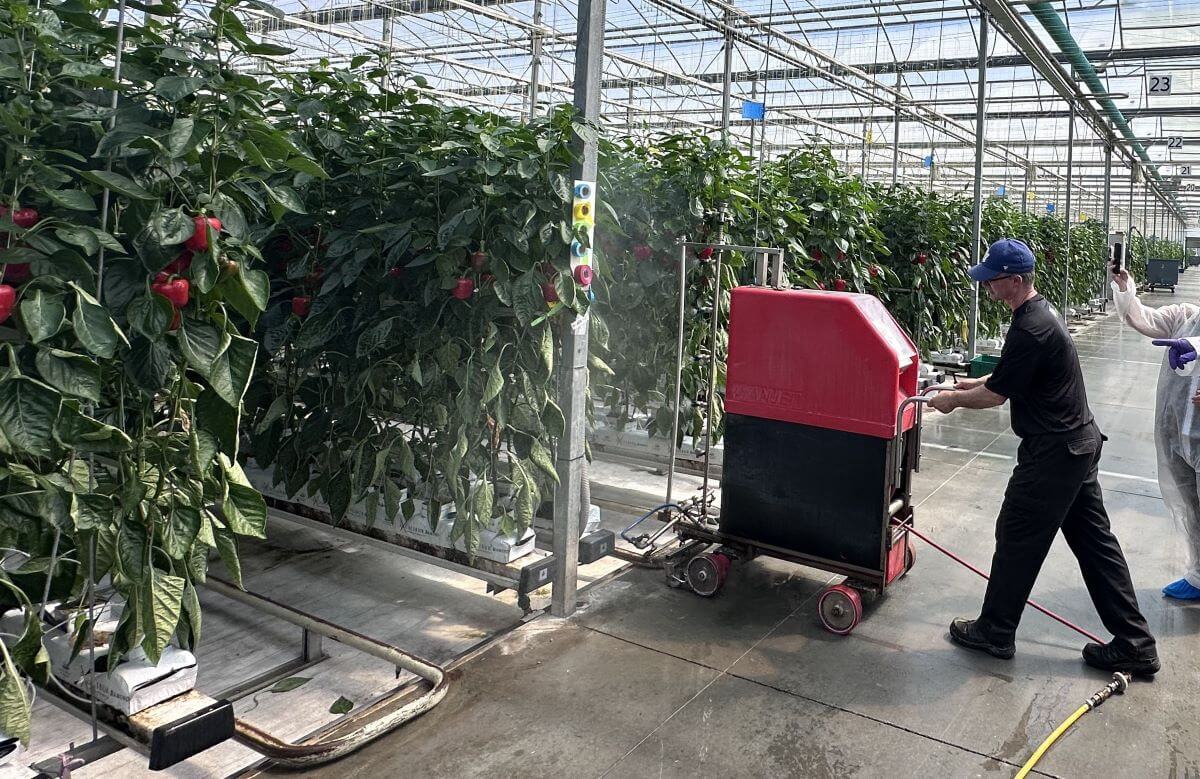
Cedarline uses semi-automatic “robot trees” (Wanjet model S55). This sprayer has a vertical, 2 m high boom with nozzle bodies spaced every 25 cm. When the crop grows higher than the boom, an extension is added to bring it to 4 m. Flange wheels allow the sprayer to ride the hot water pipes between the rows like a train on rails at a rate of 60 m/min.
The sprayer is manually placed in the row. Then it trundles along, spraying one side, until it reaches the end of the row. Then the vertical boom turns to spray the other side on the return trip, where it is retrieved and placed in the next row. The sprayer is fed from a portable tender unit via a 180 m auto-reeled hose at 200 psi. The question is, does this all work the way we assume?
4. Calibrating the sprayer
4a. Pressure
We started with pressure. If pressure is the force that causes a specific volume of spray mix to exit the nozzles at a specific rate and produces a specific droplet size and spray geometry (e.g. a cone or a fan), then it’s very important to know that it’s accurate.
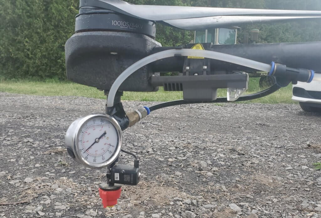
Remove the gauge with a wrench (never turn it by the face) and test it against a known gauge. You can build a test apparatus very easily. Alternately if the gauge is showing wear, such as the needle not sitting on the zero pin, or it’s opaque, or leaking, maybe just replace it without testing.
In our case, we discovered the gauge was off by 20%. Where the standard gauge read 150 psi, the working gauge read ~120 psi. Plus, the scale of the gauge was far too high. Best practice is to use a gauge rated to about double the operating pressure. This gives better resolution, and a quick glance shows if the needle is pointing straight up.
I prefer a tender system like this over a central spray tank in a header house. In systems where there is a central tank and the sprayer hoses plug in at intervals, the degree of pressure-drop increases with distance from the source. If this is you, install a regulator on your sprayer and adjust it accordingly to hold the pressure constant. In this case, the distance the spray solution travels is always constant, so the pressure doesn’t change. Best practice in either case is to install a pressure gauge on the sprayer at the end (or top) of the boom so you can confirm the operating pressure is correct.
4b. Sprayer speed
We were told the sprayer was set to travel 60 m/minute, but is that true? Certain chemistries will deposit a slick coat on the hot water pipes and the flanged wheels can slip (especially as they wear). There was obvious damage to the rubber surface of two of the flanged wheels that might have affected travel speed. We should have checked, but we didn’t. Use a timer and confirm how long it takes for the sprayer to travel to the end of the row. Don’t include turn time. If it doesn’t match your expectation, then adjust the speed until you get what you want.
4c. Boom and nozzles
Next, we explored the boom and the nozzles. The first thing we saw was that their alignment was wrong. Flat fans in ¼ turn nozzle caps will self-align on the lug to ensure each spray fan does not physically impact it’s neighbours. However, the nozzle bodies themselves can sometimes turn on the threaded boom, and they need to be realigned. We did that before removing a few tips for inspection.
Each nozzle should be oriented 10-15 degrees off vertical and parallel to one another. Here, the top one is correct, but the lower nozzle has twisted and will leave a gap in the swath.
I asked when the nozzles were last replaced and was told the sprayer arrived pre-nozzled with TeeJet visiflo 8002’s. They had never been inspected, other than when they plugged, and their rates had never been confirmed. Upon inspection we found some were physically damaged. This doesn’t mean the nozzle orifice was compromised, but it instilled doubt. You don’t always see obvious damage but know that the orifice is delicate and very precise. As it wears it gets larger (increasing flow), but more insidiously it also changes shape, altering the size of the spray droplets, which we’ve established are critical to our spray strategy.
Best practice is to test nozzle outputs at a known pressure and replace them when they are 5% off the expected rate. Unless a nozzle gets physically damaged, replace them as a set so they wear as a set. When do they wear out? It depends on the nozzle material, the nature of what you’re spraying, the pressure and the amount of time they spend spraying. Here’s a link to an article that suggests several methods for testing nozzle output. Some are cheap and slow, others are fast and expensive, but they all work.
If that’s not appealing, you can mark your tank and see how many rows you should be spraying versus how many you’re actually spraying. Ultimately, given the relatively minor expense of new tips versus the trouble of calibrating them annually, it’s often simpler to replace them at intervals. In this case it’s worth noting that the first 2 m of boom operates all season, while the extension is only added later, so they won’t all wear at the same time.
We examined and then returned the original tips to the boom for the next part of the calibration. We noticed that the gaskets were stretched (crushed). This made it hard to put the nozzles back on, so they would also need replacing.
We turned on the boom to ensure we had everything back in the right place, and noticed that when we stopped spraying, the boom slowly emptied through the lowest nozzles. That meant expensive products were left to dribble out every time the boom stopped spraying, which is wasteful. It hinted that the check valves, which are built into the nozzle bodies, were no longer working. Ideally, once the boom pressure drops below ~15 psi, each check valve diaphragm closes to prevent leaks. It also ensures the boom remains primed for the next pass. We advised that they should be replaced and to ensure the new bodies have the correct thread size. European sprayers rarely have the same thread as North American, so compatibility can sometimes be an issue.
5. Evaluating spray coverage
This is an iterative process, which means we test, evaluate, make a single corrective change, and repeat until we (hopefully) see what we want. Water sensitive paper (WSP) is a terrific tool for this process, but it has a few caveats:
It will react to any moisture, including a humid atmosphere, so handle it with gloves and don’t let it sit for too long.
The WSP surface is only a surrogate for a plant surface. Deposits tend to spread more on leaves, vegetables and fruits, but will always be smaller on the papers. So, only compare papers to other papers and infer that the actual crop coverage is better.
We really don’t know how much coverage is enough. It depends on pest pressure, product concentration and mode-of-action (e.g. contact or systemic). Generally, we like 10-15% of the surface covered with 85 deposits per cm2 on 80% of the targets. Sometimes it’s easier to imagine the pest on the paper – can it fit between the deposits?
5a. TeeJet visiflo 8002 at 200 psi
We started by establishing a baseline using their current nozzles and pressure. WSP was folded and clipped at the petiole so we could assess adaxial and abaxial surfaces. We placed them deep in the canopy so we were looking at the worst-case scenario, and then noted where we left them (use a ribbon or part of the greenhouse as a frame of reference or you’ll never find them again). We sprayed from one side, then examined them in situ, then sprayed from the other side so we could see the impact of cumulative coverage.
After spraying from both sides, we saw excessive coverage on adaxial surfaces and marginal coverage on abaxial. For those that have tools to digitally scan and assess WSP, it worked out to 31% coverage and 225 deposits/cm2 on the adaxial side, and 2% and 16 deposits/cm2 on the abaxial. In fact, the adaxial side was so saturated (>25% coverage) that I don’t trust the deposit counts because of overlaps, but there it is. This is when we brought out the nozzle manufacturer’s catalogue (which you can also find online). We found their nozzle and looked up the flow table, which shows the relationship between pressure, output rate and droplet size.
Those in greenhouses might find that their operating pressures are far higher than what is listed, but that’s no problem. Find the highest pressure and output rate listed in the table and call those “Known Output Rate” and “Known Pressure”. Now use the following calculation to extrapolate flow for a new pressure. It’s also worth knowing that higher pressure tends to mean a wider fan angle and finer spray droplets than are listed in the table:
Unknown Output Rate (gpm) = Known Output Rate (gpm) × (square root of New Pressure (psi) ÷ square root of Known Pressure (psi))
In this case, at 200 psi this nozzle should produce 0.45 gpm. If we go up one size from the yellow 02 tip to a larger blue 03 tip, we can produce a similar flow but using only 100 psi. This would put less strain on the system, but it would also make droplets larger, fewer and perhaps slower.
5b. TeeJet visiflo 8003 at 100 psi
We tried the 8003 at a lower pressure and saw that the deposits were obviously larger on the adaxial side, and not saturating, which is good. However, we saw insufficient deposit density on abaxial, which was a deal breaker.
5c. TeeJet visiflo 8003 at 200 psi
We left the blue 8003s and brought the pressure back up to 200 psi. Now the flow was increased to 0.67 gpm, and the droplets were finer, more plentiful and moved a lot faster. The adaxial surface went back to excessive coverage, but perhaps not as bad as with the 02s. The abaxial deposit density was improved, but still not sufficient. You can see the results of the three trials in the photo below. Go counter-clockwise from 1 (at bottom right) to 3 (at top).
5d. TeeJet twinjet TJ6011003 at 200 psi
It was time for a radical change. We replaced the single flat fan geometry with twinjet flat spray nozzles (TJ60-8003). We tried this because we’ve tried it in the past and it worked well. We retained a blue 03 rate, so we still produced 0.67 gpm at 200 psi. This nozzle also retained the 80° fan angle, but created two of them at 60° to one an other. This would change the spray trajectory, creating new opportunities for droplets to align with the targets. Perhaps most importantly, the twin fan nozzles would produce finer droplets than their single fan cousins, increasing the odds and perhaps and creating more “wind”.
We saw far less differential between abaxial and adaxial surfaces, with deposit density greatly improved on both surfaces. While the adaxial face showed larger deposit diameters, they were close enough to require close inspection to determine which side was which; Coverage was more uniform, with no drenches and no misses. By the numbers we saw 34% and 523 deposits/cm2 on the adaxial side (again, hard to trust the counts here because of overlaps arising from >25% coverage) and 19.5% and 400 deposits/cm2 on the abaxial. We had a winner.
It’s also worth noting that every time we sprayed, we observed the deposit on the fruit and leaves. None of the sprayer configurations caused run-off (e.g. drip points on the bottom of the fruit or tips of the leaves), which would suggest we were not using an excessive volume. Look closely at the following two pictures to see the beads of water and how they deposit. They look great.
We also watched to see if spray passed through the row into the next alley. A little puff here and there is fine, because it meant the spray was reaching the far side of the row. However, spray that blows through the row excessively is wasted becuase it misses the target row and ends up on the greenhouse floor.
Epilogue
We were pleased with the result of half-a-day’s effort. We left our hosts with some homework:
Change the pressure gauge to one that is accurate and spans to 400 psi.
Replace all nozzles and gaskets and ensure they are properly oriented.
Time the sprayer to confirm travel speed is what they assumed.
Using the known speed, pressure, and boom output, do the math to account for the fact that they would now be spraying a higher volume than they were. This will change how much product they put in the tank.
Watch the crop closely to ensure these changes do not compromise crop protection.
Everyone learned a lot from our day together. Cedarline said they would calibrate their other sprayers using this process. They are even going to try a set of yellow 02 TwinJets to see if they can achieve sufficient coverage at their current pressure, which would mean they can continue to mix product at the same concentration. Those are pretty small orifices, guys, so watch out for plugged tips and good luck!
Hopefully this inspired you to look critically at your own operation and to follow these steps to calibrate and optimize your crop protection practices. Happy Spraying.
Everyone here had helpful ideas during this process. Calibration is a team sport so make sure both your operators and managers are involved. Left to right: Ryan Bezaire – OMAFA Summer Student; Paul Brooks – IPM Specialist, Cedarline Greenhouses; Jason Deveau – Application Technology Specialist, OMAFA; Jimmy La Rosa – Operations Manager, Truly Green Farms / Cedarline Greenhouses; Richard Robbins – Technical Representative, Plant Products; Cara McCreary – Greenhouse Vegetable IPM Specialist, OMAFA
Calibration is a fundamental step in any spray application. To apply the correct product rate, we need to know how much liquid per unit land area is deposited under the sprayer.
To conduct the calculations, either manually or through the drone software, we need to know the width of the spray swath. This task requires the operation of the sprayer under typical conditions, some kind of sampler capture the spray deposit, and a means of quantifying that deposit so the spray pattern becomes apparent. Here’s how we do it:
1. Confirm the accuracy of the flow meter
Drones don’t typically report the spray pressure of the spray mix. Instead, they report the flow rate using a built-in flow meter. The drone maintains the desired application rate by using the flow rate to adjust pump speed and engage nozzles over a range of travel speeds. Because everything depends on the flow meter, its accuracy needs to be verified.
Fill the spray tank with clean water and flush all the lines.
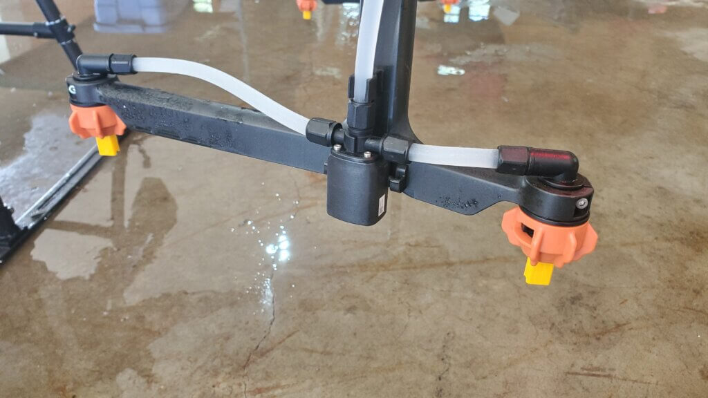
Install nozzles required for task, ensuring all nozzles are identical and in good working order.
Nozzles installed on DJI T20 drone.
Select the nozzle size you installed on the spray monitor.
Purge the air from the system.
Activate the spray and wait for the flow rate to stabilize on the spray monitor. This may take a few moments.
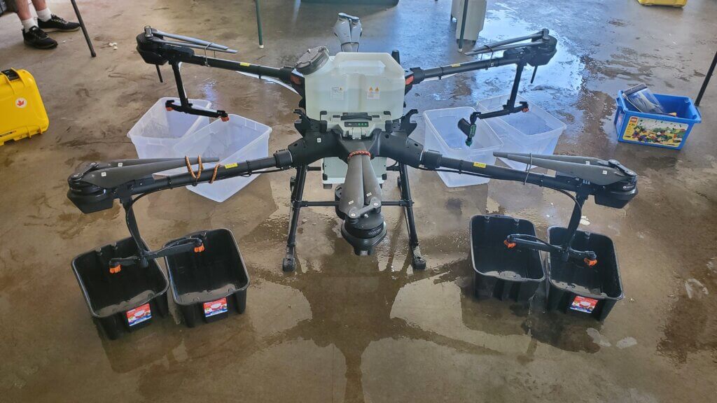
With the nozzles flowing, place collectors under each nozzle and collect the spray liquid for a fixed time, say one minute.
Capturing spray during flow meter calibration.
Ensure the collector catches all the spray. Buckets often create turbulence. Rotary atomizers make this more difficult.
When the time elapses, remove the collectors and then shut off the spray.
Unless the shutoff is very fast and positive, leaving the collectors in place during shutoff can introduce error as the flow diminishes.
Confirm that the volume collected from each nozzle was identical, and that the flow rate reported by the drone flow meter is accurate.
Repeat to ensure consistency.
Use of a Spot-On digital calibrating cup ensures that all spray is captured and it also reports the volume instantly.
2. Measure the swath width
Spray swath width is variable. For a measurement to be relevant we must evaluate spray deposition under environmental conditions that are similar to the planned spray operation, as well as use the same operational settings such as altitude, travel speed, nozzle choice, and application volume.
Spray samplers are positioned along the ground, perpendicular to the flight path. We use water-sensitive paper (WSP) because it’s readily available, fast and easy to use, and the deposits can be analyzed visually or using simple apps that calculate coverage. We create a sampling line of WSP positioned a 1 m intervals (or maybe 0.5 m for narrow swaths). The samplers should extend to twice the expected swath width to account for any swath displacement from sidewinds.
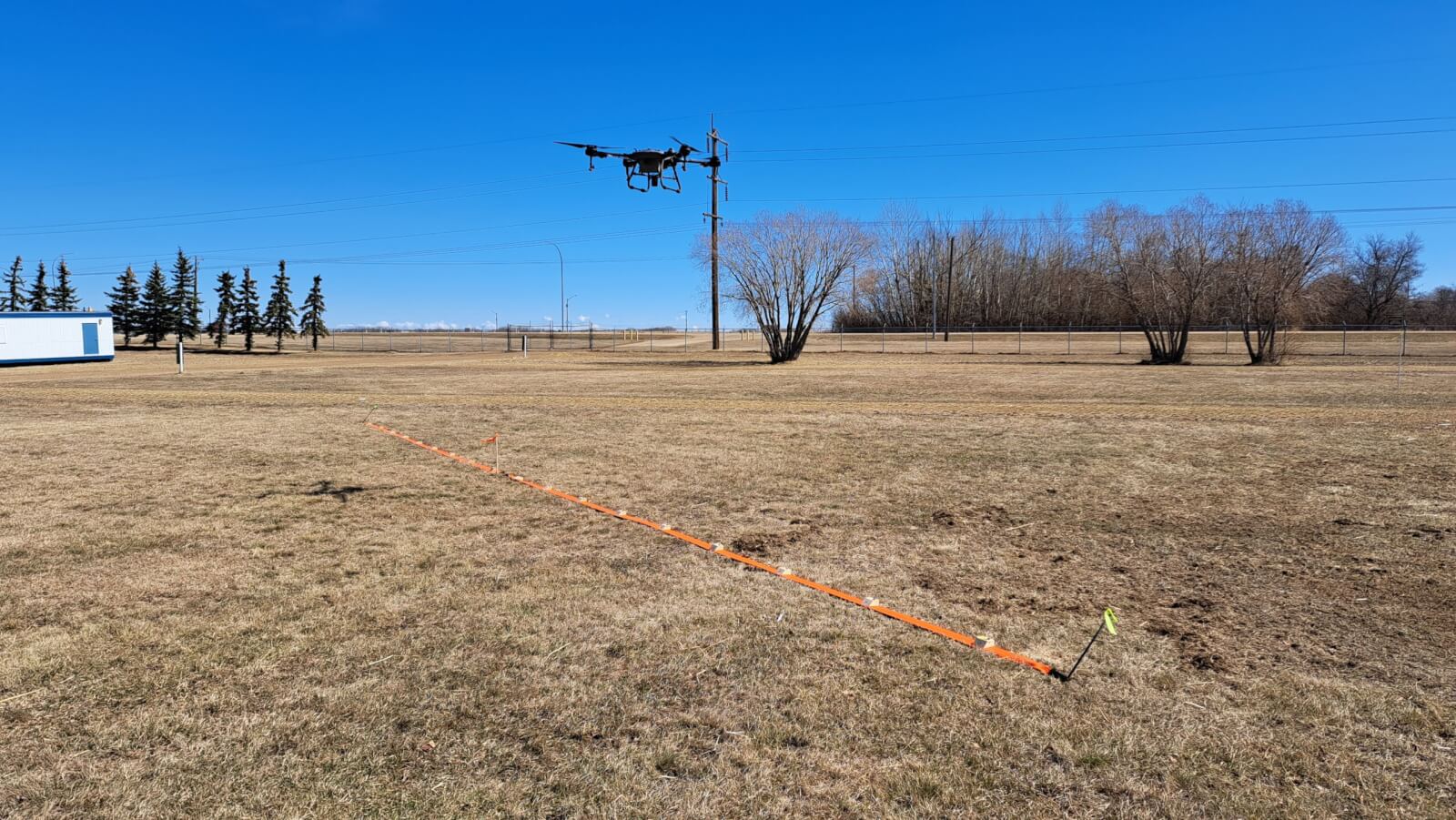
Choose a day with light, consistent winds.
Find an open space free of obstruction in the direction of the prevailing wind.
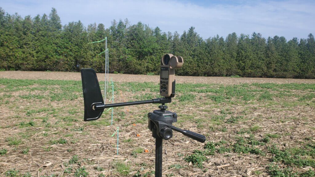
Install a weather station to document conditions during flight.
A Kestrel 3550AG or 5550AG wind meter can record weather data and download to a phone via Bluetooth.
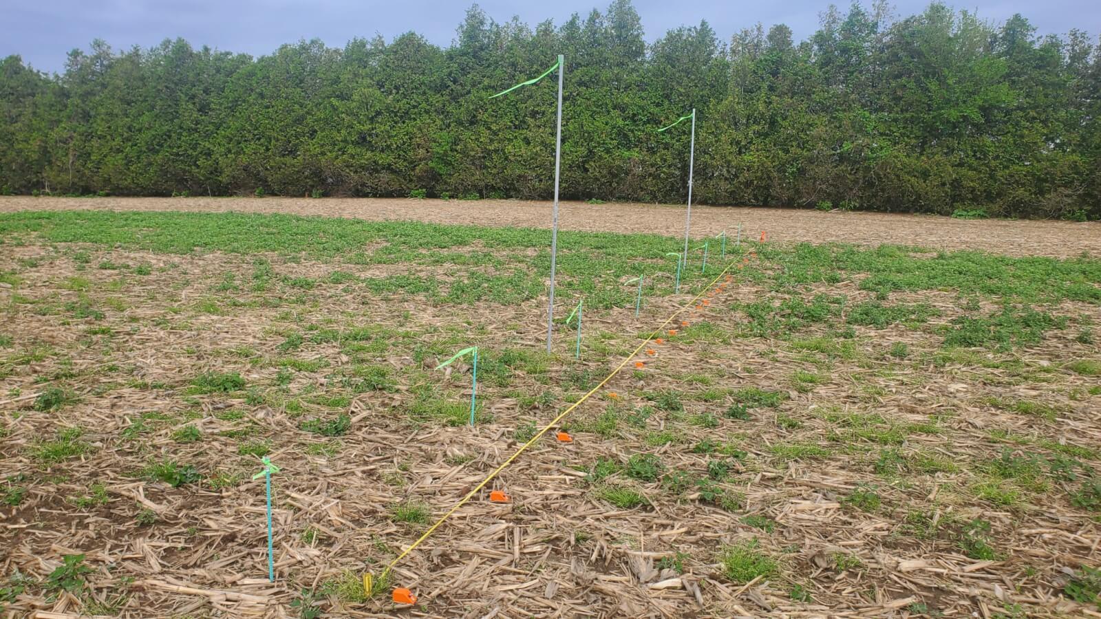
Mark an approximately 200 m long flight line into the prevailing wind direction by placing wire flags every 50 m.
At the 150 m mark, use wire flags to centre a sampler line perpendicular to the flight path. Sampler line length should be about twice the expected swath width.
Swath sampling line
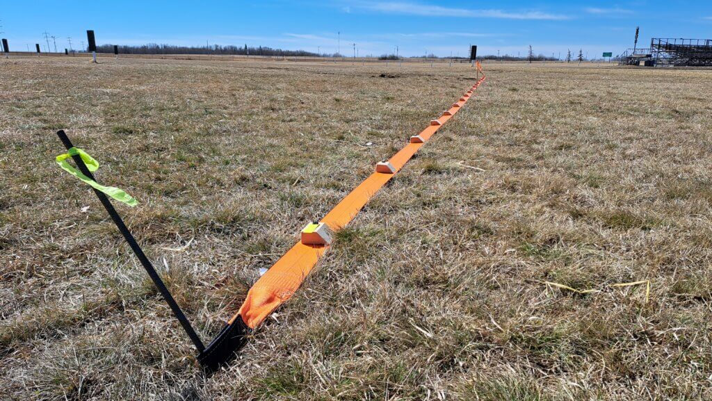
Wooden blocks with paper clips can be used to secure WSP at regular intervals along the sampler line.
Wooden blocks attached to a 4″ tow strap allows for easy setup and movement of sampling line.
Fill the drone 1/2 full.
Manually fly the drone along the entire flight line. The spray pressure, flow rate and altitude of the drone should be stable before it reaches the sampler line. This may take 25 meters or more depending on drone model, flight speed and drone weight.
Fly 50 m past the sampling line without any drone maneuvering to avoid affecting the deposit.
Land the drone and walk along the sampler line.
Note the deposits in the central region. Walk along line as the deposits taper off, looking for deposits that are approximately 50% of the average central deposits.
Water-sensitive paper following a drone application.
Estimate the distance between these deposits on both edges of the swath. This is the estimated swath width that can be entered for the second flight.
Replace the WSP with a fresh set, refill the drone to 1/2 full, and repeat the flight two more times.
Other methods perform a more advanced assessment by analyzing the entire swath, and not just intervals. These methods use dyes and dedicated hardware to quantify the deposits along strings or paper samplers.
The Swath Gobbler documents swaths at high resolution using lengths of 3″ bonded receipt paper, food grade dye, and a digital scanner.The Application Insight LLC Swath Gobbler scanner in action.
3. Analyze the Pattern
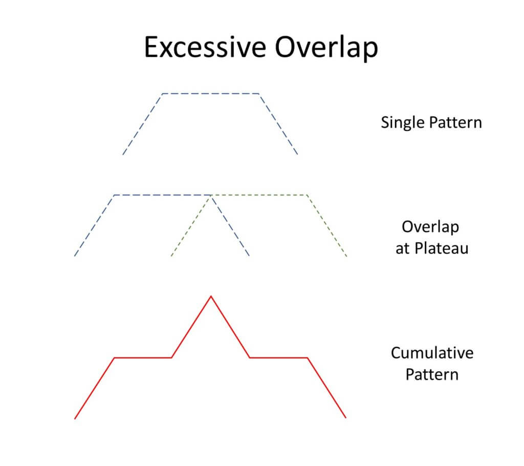
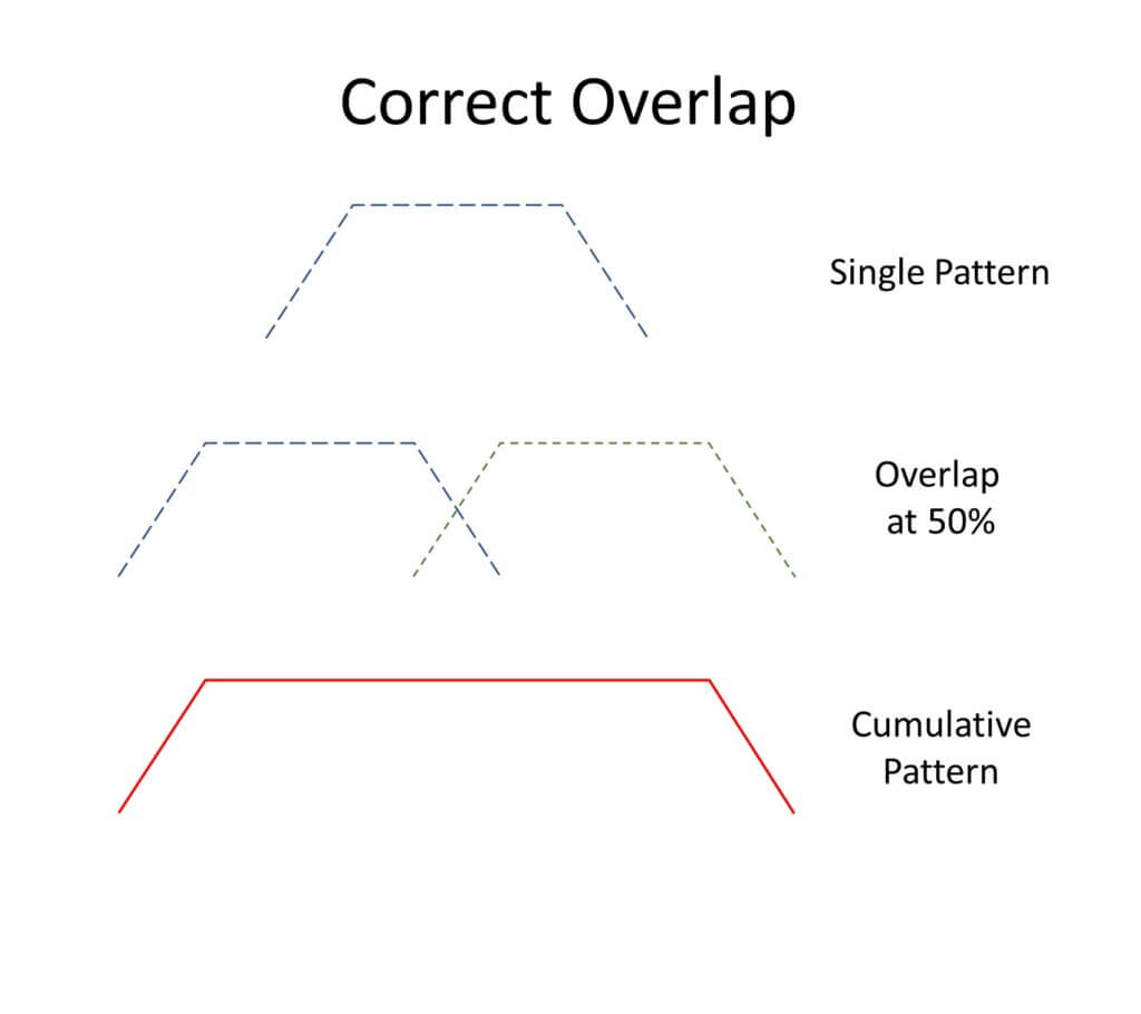
The nearest approximation for drone swathing is that of a manned aircraft. The spray pattern of an aircraft is tapered, meaning the highest deposition is near the centre of the swath, and the edges of the swath fade to zero deposit. In order to achieve consistent coverage, we need the edges of the spray swath to overlap so the cumulative coverage at the edges is closer to that in the centre. Too little overlap leaves gaps and too much overlap results in excessive deposit.
Insufficient overlap creates gaps in coverageExcessive overlap results in over-dosing and wasteCorrect overlap is necessary for efficient and effective application.
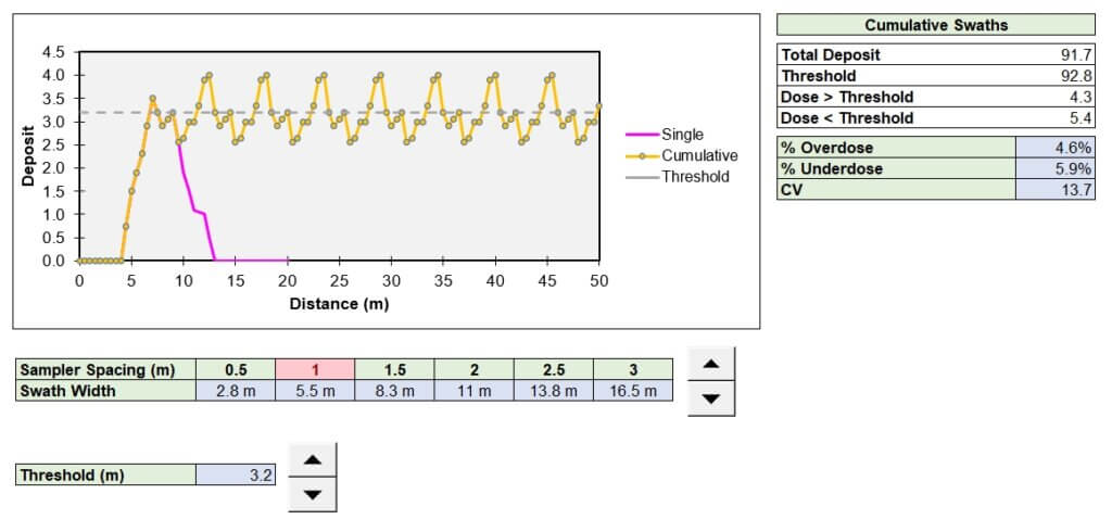
Deposits from drones can be highly variable. The challenge is to find an overlap distance that minimizes this variability, minimizes both over- and under-application, and maximizes swath width. Download a copy of our Excel spreadsheet to help you with this process.
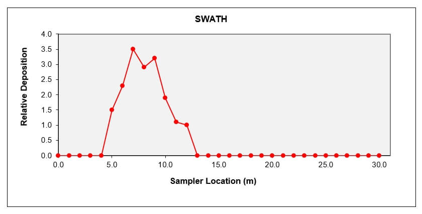
The first step is to estimate a reasonable average deposit, called “Threshold”. Graph the deposits from each sampler, and estimate a point on the Y axis (Relative Deposition) that represents the average maximum deposit. This could be the maximum value of the plateau, or a midpoint between the maximum and a nearby dip. This is the Threshold. We then take 50% of this estimated average deposit, and find the two distances on the X axis (Sampler Locations) that intersect the curve at these points. The distance between these two points is our first estimate of the swath width. If two adjacent swaths are spaced so the edge of one overlaps 50% with the next, the overall cumulative deposit should be relatively even.
The coverage information from each sampler location is graphed to create a deposit pattern.
We can alter the amount of overlap to improve the apparent uniformity, but be cautious. For example, even though we can often improve the uniformity by narrowing the swath width, this can add deposit to the area under the drone and raise the overall deposit amount. Plus, the narrower swath also lowers the productivity of the drone. Use the Excel model to establish a swath width that has the lowest variability (Coefficient of Variability or CV) AND results in a balance between over- and under-dosing.
The amount of overlap is adjusted to minimize variability (CV) and both equalize and minimize over- and under-dosing.
4. Recognize the factors that influence swath width
Operational use case affects swath width
Swath width is affected by altitude, speed, water volume and spray quality. Generally, higher altitudes, lower volumes, and finer sprays will result in a wider swath. Unfortunately, the same configuration also results in greater drift. It is recommended that swath widths be determined for each spray volume and nozzle arrangement that will be used.
Drones will be applying low water volumes and this requires a critical assessment of coverage to ensure the deposit density is sufficient to achieve the desired result. A low volume will require a finer spray for minimum coverage to be realized. Coarser sprays that reduce drift and evaporation will need higher water volumes and result in narrower swaths. Significant time may need to be invested to understand the effects of operational settings and environmental conditions on spray deposit uniformity and swath width.
Effective Swath Width and the Agronomic Use Case
The relatively sparse coverage at the extremes of the measured swath width may be insufficient to elicit the desired biological result. The Effective Swath Width (ESW) represents the segment of the total swath width that results in pesticide efficacy. In some use cases, the two widths can be similar, but typically the ESW is only a fraction.
The difference is influenced by the “Agronomic Use Case” which includes factors such as:
Spray mix rheology (i.e. the interaction of spray mix viscosity and atomizer design on droplet size)
Minimum effective dose: This is a complex relationship between coverage, spray mix concentration and pesticide mode-of-action that results in an effective result while minimizing the environmental impact.
Target location (e.g. a pest within a dense canopy or a weed on relatively bare ground)
Taken collectively, research has shown a 20-30% reduction in ESW for corn, wheat and soybean fungicide applications compared to swaths measured on open ground. Conversely, herbicides sprayed on bare earth or sparse vegetation can produce an efficacious response 20% wider than the measured swath width. The impact of agronomic use case on ESW must be considered during mission planning.
Additional pointers
Here are a few tips and tricks to help you be successful when calibrating your drone.
Drone patterns will have deposit peaks and valleys in the central region. Repeated runs are needed to confirm that these are real and persistent. If so, then adjustments in flying height, spray quality, or water volume may be needed to eliminate them.
The absence of pressure gauges on drones can be corrected by installing an analog gauge in-line with one of the spray nozzles. If may be necessary to mount an auxiliary camera on the drone to record this gauge. We have observed strong fluctuations in spray pressure, particularly on starting a spray swath, that were not reflected in the reported flow rate.
A pressure gauge can be plumbed into a drone without affecting flight behaviour. A camera is trained on it to read pressure during a flight.
Many drones have the option of recording the flight screen during a mission. This will provide a record of the performance of the drone, and can be valuable should performance problems arise.
Although swath width calibration is done by flying into a headwind, the actual spray application should be done with a side wind. Start at the downwind edge of the field and turn into the wind. The drone is symmetrical and the tapered spray patterns should equalize the deposits. Alternately, flying into a headwind and returning with a tailwind can alter the aerodynamics of the spray deposition process, alternating between a wider and more narrow swath width, respectively.
Drone spraying will walk a razor’s edge of sorts – there is little room for error when using scant water and fine droplets. Getting the basics right has never been more important.