North American product labels may or may not include carrier volume recommendations. When they do, it could be based on a two-dimensional value like the planted area, or perhaps on row length which is more appropriate for trellised crops that form contiguous hedge-like canopy walls. Volume may also be tied to product concentration, which sets minimum and maximum volumes based on product rates. Or, more commonly, volume recommendations take the form of vague guidelines such as “Spray to drip” or “Use enough volume to achieve good coverage”.
In all cases, spray efficacy and efficiency can be greatly improved by dialing-in the carrier volume to optimize coverage uniformity and reduce off-target spraying. This is easier said than done because the optimal spray volume is case-specific. It depends on a complicated relationship between:
- Weather conditions (E.g. temperature, humidity, wind speed and direction)
- Sprayer design (E.g. air handling, droplet size and flow distribution over the boom)
- Traffic pattern (E.g. every row or alternate row)
- Product chemistry (E.g. mode of action and formulation).
- Target (E.g. Crop morphology, planting architecture)
It is the final variable, the nature of the target, which is the focus of this article. To learn more about the other variables, grab a copy of Airblast101.
The plant canopy and planting architecture dictate volume
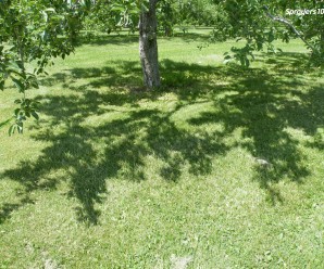
Quite often, the target in airblast applications is the plant canopy. The plant canopy is the collective structure containing all plant surfaces. This could be the foliar portion of a single pecan tree, a panel of grapes, or a bay of container crops. The planting architecture describes how those canopies are arranged on the planted area. If we consider the canopy and architecture geometrically, we can make relative statements about the volume required when all other variables are equal.

| Geometric Characteristic | Relationship to Carrier Volume (per unit planted area) |
| Row Spacing | The greater the row spacing, the less volume needed. |
| Plant Spacing | The greater the plant spacing, the less volume needed. This assumes gaps between the canopies (I.e. not a contiguous hedgerow). |
| *Canopy Depth | The greater the canopy depth, the more volume needed. |
| *Canopy Width | The greater the canopy width, the more volume needed. |
| *Canopy Height | The higher the canopy, the more volume needed. |
| Canopy Density | The denser the canopy, the more volume needed. |
Canopy density
Let’s focus on a single plant canopy. Research has demonstrated that with the possible exception of canopy height, canopy density has the greatest influence on optimal sprayer settings.
Density describes the amount of matter inside a canopy relative to the volume of space it occupies. The denser the canopy, the more surface area there is to cover and the more difficult it is for spray to penetrate.
While air handling plays a significant role in improving coverage, a denser canopy will almost always require a greater carrier volume.
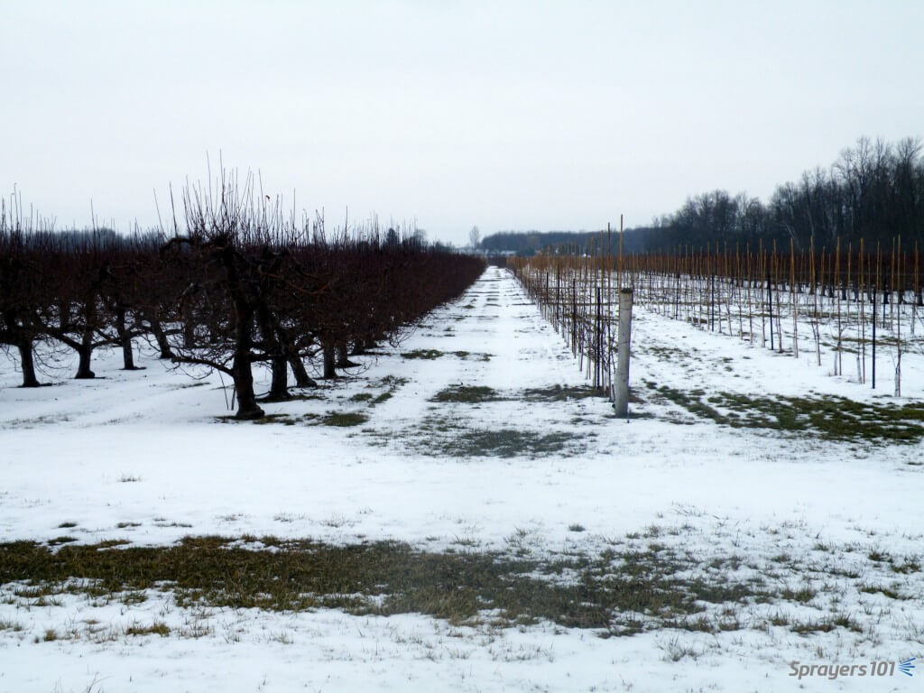
For most perennial crops, canopy density changes over the growing season. The influence of age and staging on canopy size and density will depend on the crop variety, plant health and canopy management practices. The practical implication is that as the canopy grows and fills it typically warrants an increase in spray volume.
As illustrated in the figure below, the volume used should reflect the current stage of canopy development. If a volume suitable for the densest and largest stage of development is used all season, it will create a great deal of waste early in the season. However, if volume is increased incrementally to reflect canopy growth, a better fit between coverage and volume will minimize waste.
Note that volume is increased around petal fall, but the fit could be improved with more increments. Caution is advised to ensure the volume is raised (if required) prior to immediate need, particularly during key developmental stages like bud break or bloom where fungicide coverage is critical.

There are exceptions to this rule. Many nursery crops and mature evergreens often do not require changes to volume. High density apple orchards may or may not require an increase in volume. Early in the season, sparse canopies have low profiles that result in very low catch efficiencies. In other words, a great deal of spray misses the target.
The amount of waste is a function of the application equipment design and the weather conditions. Most low-profile axial airblast systems envelop the target in spray with limited means of reducing air energy sufficiently, or to turn off the spray between trees.
Further, sparse canopies do not restrict wind, which means ambient wind speed tends to be higher early in the season compared to when the trees become wind breaks. This creates a drift-prone situation and higher volumes are often used to compensate for the loss. The collective result is that excess spray volume is inevitable early season.
As the canopies fill, the wind is reduced and catch efficiency increases, so trees intercept more spray without having to raise volumes. This balance eventually tips, however, and an increase in volume may be advisable.
Watch the following video to see the impact of using excessive spray volume (and poor air adjustment settings) in a young cherry orchard. The waste becomes particularly apparent at ~43 seconds when the sprayer passes in front of the woods and the plume can be seen with higher contrast.
While some loss is inevitable in such a sparse canopy wall, this situation could be improved by using less carrier volume, larger droplets, the correct air settings, canopy-sensing optics and/or a tower or wrap-around sprayer design.
Adjusting spray volume sprayer settings to reflect the canopy can save money and reduce environmental impact during early-season applications and in young plantings. Mix the tank as you normally would to maintain the pesticide concentration on the label, but adjust the sprayer output to match the plant size.
Performed correctly, you will be able to go further on a tank without compromising efficacy. This crop-adapted spraying method and the relationship between spray volume, concentration and dose are described further in this article and this article.
Estimating volume from canopy geometry
It is challenging to decide on an appropriate spray volume. Many operators resort to historical or regional practices and do not make adjustments to reflect their specific situation. Others refer to models such as Tree Row Volume (a.k.a. Canopy Row Volume) which relates canopy volume per planted area to spray volume.
In this case, catch efficacy is expressed as a coverage factor, which is determined through experimentation specific to the crop, environment and sprayer.
Tree Row Volume = (Avg. Canopy Height × Avg. Canopy Spread × Planted Area) ÷ Row Spacing
Spray Volume = Tree Row Volume × Coverage Factor
In New Zealand, coverage factors for dilute applications to deciduous canopies range from 0.07 to 0.1 L/m3 (0.00052 to 0.00075 US gal/ft3) or 71 to 100 ml/m3 (0.067 to 0.096 US oz/ft3). The range captures variation in canopy density and any product-specific coverage requirements. Oil sprays, for example, require more surface coverage than most products. While closer to “the truth”, the Tree Row Volume method is still only an estimate.
If the operator has no prior experience with the crop or the sprayer and wants a sanity-check on their estimated spray volume, we propose the following guidelines for full canopy dilute application to mature crops using every-row traffic patterns. The volumes may seem high, but recognize we have selected a very challenging scenario.
- Small canopies (E.g. bush, vine, cane, high-density fruiting wall): 500 L/ha (55 US gal./ac.) to 1,000 L/ha (110 US gal./ac.).
- Medium canopies (E.g. tender fruit, pome): 750 L/ha (80 US gal./ac.) to 1,250 L/ha (135 US gal./ac.).
- Large canopies (E.g. tree nut, citrus): >2,000 L/ha (214 gal./ac.) and up tp 7,000 L/ha (748 US gal./ac.).
- For sprayer operators that think in 100 m row lengths, consider 20 L volume per 100 m row length per 1 m canopy height.
Further Resources
No matter the approach to determining spray volume, it is imperative that coverage is assessed. It is amazing what we ask of airblast sprayers. Read this short article for some perspective on the coverage we hope to achieve from a given spray volume.
We propose the use of water-sensitive paper to assess spray coverage. We describe its use and evaluation in detail in this article, this article and in this article.
Dialing-in an optimal spray volume is an iterative process that requires careful observation and keeping records on what works and what doesn’t for your specific operation.
Jon Clements (University of Massachusetts) has noted special considerations when it comes to establishing effective volumes for plant growth regulators that go beyond this article. You can explore the concepts in this 2021 factsheet (Spray Mixing Instructions – Considering Tree Row Volume) by Terence Robinson and Poliana Francescatto (Cornell University) and Win Cowgill (Professor Emeritus, Rutgers University).
Finally, if you really want to get lost the weeds, check out this video recorded in 2021. I had an opportunity to learn from pros like Dr. Terence Bradshaw (University of Vermont) and participants from the Great Lakes region. They’ll tell you all you ever wanted to know about Tree Row Volume. Settle in!
Thanks to Mark Ledebuhr of Application Insight LLC for his contributions to this article.