The scuttlebut on coffee row is that acidifying a spray mixture improves its efficacy. There are also claims that pesticides break down in the sprayer tank if the pH is too high.
But it’s not that simple. Low pH has a strong impact on pesticide solubility, and that means mixing and cleanout are affected. Acidifying the mixture can have profound negative effects for many products.
It’s important to know what you’re doing.
What is pH?
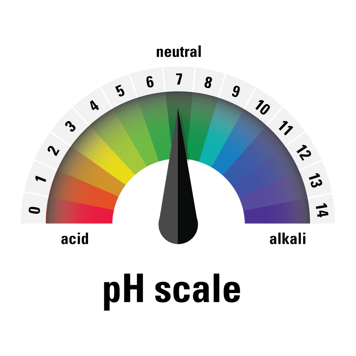
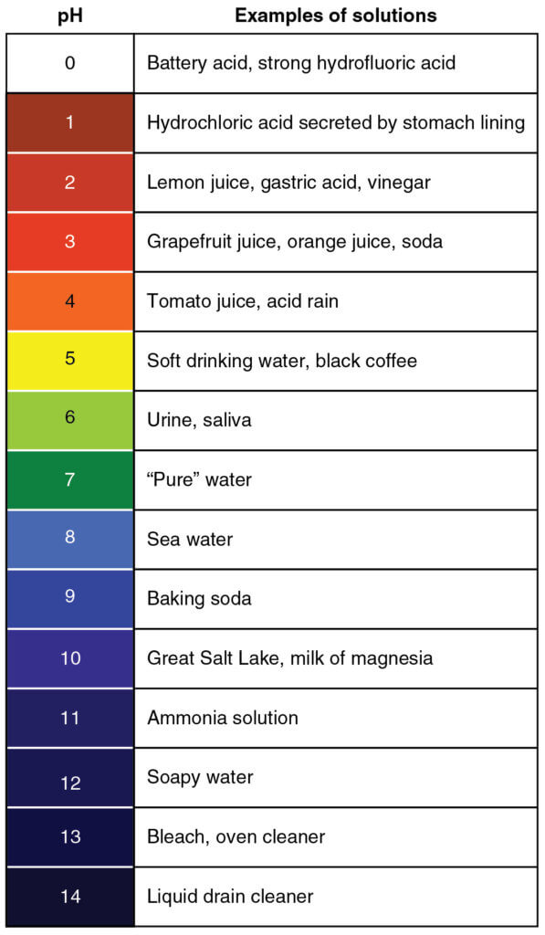
pH is defined as the negative log of the molar concentration of hydrogen ions in a water-based solution. The more abundant the hydrogen, the lower the pH. It’s a log scale, so every unit of pH refers to a 10-fold change in the concentration of hydrogen ions.
Both very low (acidic) or very high (basic) pH can be caustic. But having a low or high pH doesn’t mean it will burn your skin or clothes right away, it might just be a bit unpleasant. But at the extreme ends, protection is needed.
Why is pH Important in Spray Mixtures?
In spraying, the main effect of pH is on the pesticide’s solubility. Solubility matters when mixing and becomes important during cleanout as well.
A minor effect on pH, at least for herbicides, is on chemical breakdown, usually through hydrolysis, when the pH is too high. The effect on breakdown is rarely meaningful during any given spray day, but may play a role if a spray mix is stored overnight or longer.
The Basics: Strong vs Weak Acids
Strong acids like hydrochloric acid (HCl) ionize completely in solution. When added to water, only H+ and Cl– are present, there is no HCl. The water’s pH does not affect solubility of a strong acid.
But weak acids do not completely ionize. The water pH affects the degree of ionization and therefore solubility.
Most herbicides are weak acids. A weak acid is one that does not dissociate completely in solution. A typical example of a weak acid functional group is carboxylic acid (-COOH). In solution, compounds with a carboxylic moiety exist in an equilibrium, with some as -COOH (containing the hydrogen, also called “protonated”) and others as -COO– and H+. In the dissociated form, the acid is more water soluble than in its protonated form due to the negative charge that makes it ionic.
Weak acids have a dissociation constant known as the pKa. When the solution is at the molecule’s pKa, the acid is 50% dissociated. When the solution has a lower pH than the pKa, there is less dissociation and the protonated forms of the molecule dominate. That has two important implications for herbicides.
- the molecule becomes less water-soluble at lower pH
- the molecule has fewer opportunities to interact with positively charged items
pH Dependent Solubility
Water-solubility is a two-edged sword. On the one hand, having a highly water soluble product makes it easier to dissolve in water. This pays dividends when mixing a batch or cleaning a sprayer because a product formulated as a solution will easily go into a true solution and will stay mixed. Examples are glyphosate, glufosinate, and salts of 2,4-D, MCPA, and dicamba.
On the other hand, most pesticides need to enter a plant to reach their site of action. And a plant cell, with its waxy cuticle and oily membranes, creates an effective barrier for water, and for water-loving molecules dissolved in it. As a result, a formulation that allows the water-soluble product to interact with an oily barrier is needed.
The products that can do this are surfactants. Acting like detergents, surfactants have regions in their structure that are oil-loving (lipophilic) and other regions that are water-loving (hydrophilic). Surfactants can therefore bind to both oil and water and provide a bridge for water-soluble products across oily barriers.
That’s also one of the reason that the most water-soluble products such as glyphosate and glufosinate contain a lot of surfactants in their formulation, reducing the concentration of active ingredient in the jug and possibly leading to foaming with agitation.
Pesticides have a wide range of solubilities, and for some, water pH will play an important role. Below is a table of some water solubilities of selected herbicides.
| Solubility (ppm) | |||||
| Trade Name | Active Ingredient | Mode of Action Group | pH ~ 5 | pH ~ 7 | pH ~ 9 |
| Select | clethodim | 1 | 53 | 5,450 | 58,900 |
| Ally 2 | metsulfuron | 2 | 550 | 2,800 | 313,000 |
| Express | tribenuron | 2 | 48 | 2,040 | 18,300 |
| Pinnacle | thifensulfuron | 2 | 223 | 2,240 | 8,830 |
| Everest | flucarbazone | 2 | 44,000 | 44,000 | 44,000 |
| Simplicity | pyroxsulam | 2 | 16 | 32,000 | 13,700 |
| Frontline | florasulam | 2 | 0.1 | 6 | 94 |
| Varro | thiencarbazone | 2 | 172 | 436 | 417 |
| Raptor | imazamox | 2 | 116,000 | >626,000 | >628,000 |
| Pursuit | imazethapyr | 2 | 2,570 | 12,870 | 7,500 |
| 2,4-D | 2,4-D salt | 4 | 29,934 | 44,558 | 43,134 |
| dicamba | dicamba salt | 4 | >250,000 | >250,000 | >250,000 |
| Roundup | glyphosate | 9 | >500,000 | >500,000 | >500,000 |
| Liberty | glufosinate | 10 | >500,000 | >500,000 | >500,000 |
| Heat | saflufenacil | 14 | 30 | 2,100 | >5000 |
| Distinct | diflufenzopyr | 19 | 63 | 5,900 | 10,550 |
| Infinity | pyrasulfatole | 27 | 4,200 | 69,100 | 49,000 |
Compare the solubility at pH 7 to that at pH 5. For most of these herbicides, water solubility is worse at lower pH. That is because they are more protonated and become more lipophilic.
I’ve placed a lot of Group 2 products in this table because those products are most often implicated in tank cleanout issues. All Group 2 products in this table, with the exception of Everest (flucarbazone-sodium) have lower solubility at pH 5 than they do at pH 7. For some, like pyroxsulam and floarsulam, it’s a big change. Those products, when acifified, are prime candidates for poor mixability and poor cleanout.
When it comes to dicamba, low pH has another side-effect. It makes the molecule more volatile, increasing danger to sensitive plants nearby. For that reason, acidification of dicamba in its Xtendimax and Engenia formulations is not permitted.
Note that the Group 4 examples, 2,4-D salt and dicamba salt, as well as glyphosate and glufosinate, are highly water-soluble and pH has very little effect on that.
Particularly for glyphosate, the claim that it becomes more oily at low pH and will therefore be taken up more easily, is not supported by these data. Considering that the most acidic pKa for glyphosate (it has four acidic groups) is 0.8, pH would need to be much lower for any noticeable impact on oilyness.
Tank Mixability
Given today’s environment of herbicide resistance, applications with multiple mode of action tank mixes are very common. Acidifying a spray mix to benefit one herbicide may create problems for its tank mix partners.
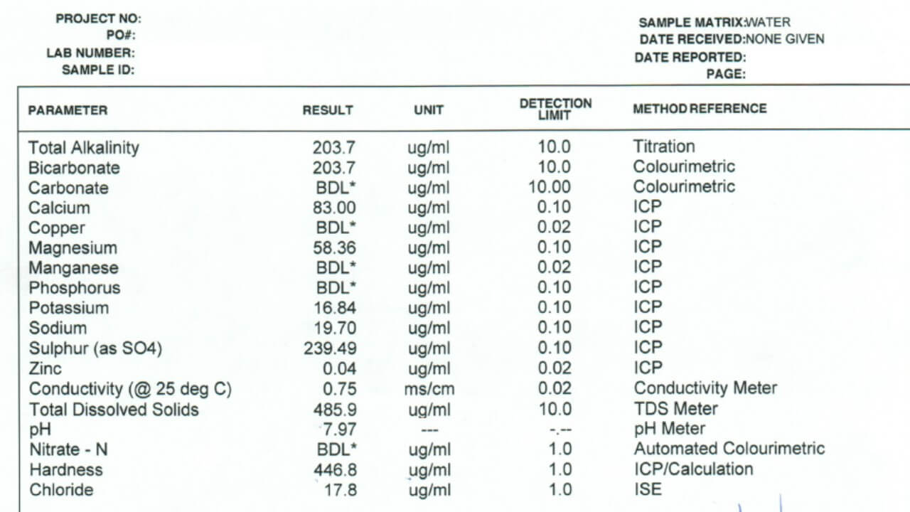
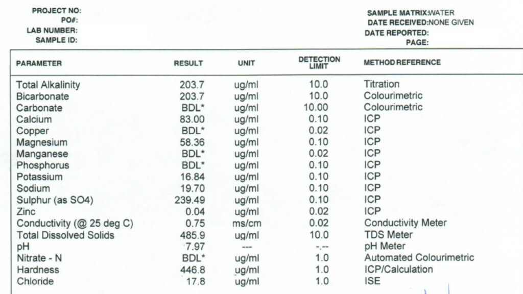
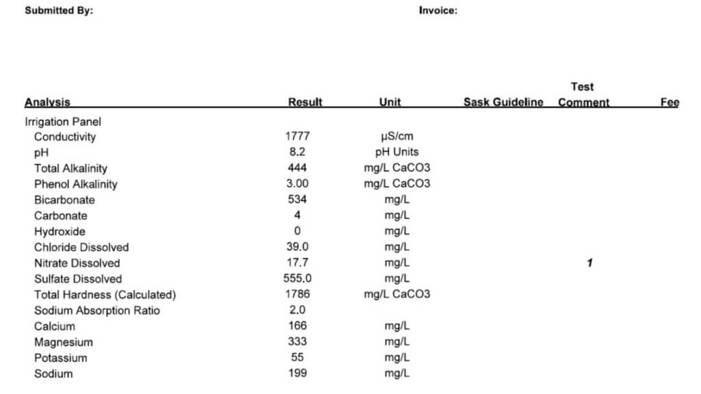
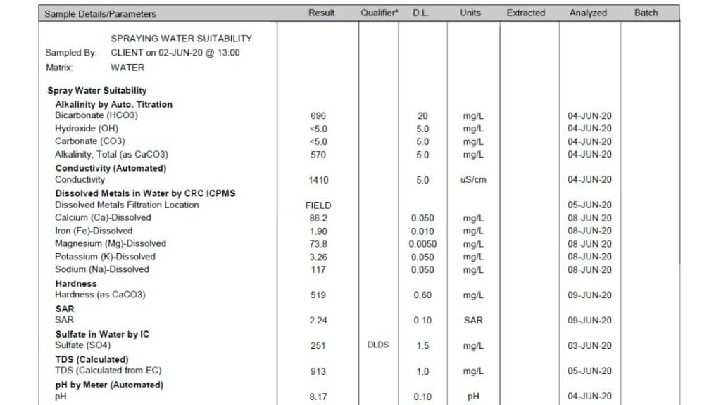
If there is a concern that spray water is too alkaline, it is recommended that the pH of the finished spray mix be measured. Since many herbicides are weak acids, they will lower the pH of the mixture by themselves. For example, the addition of glyphosate to water with pH 7.5 will drop the pH to about 5 or so, depending on the water’s buffering capacity.
As a result, glyphosate tank mix partners that are pH sensitive may suffer in the presence of glyphosate, and pH may actually need to be raised.
pH Dependent Half-life
Herbicides
There are a lot of claims that pesticides break down rapidly in alkaline spray water. And yet, in my career working primarily with herbicides, I do not recall this ever being a problem in practice.
Below is a table of herbicides for which I could find half-life information, with the help of this comprehensive list produced by Michigan State University.
| Product | Active ingredient | Half Life |
| Atrazine | atrazine | More stable at high pH |
| Banvel | dicamba | Stable at pH 5 – 6 |
| Bromoxynil | bromoxynil | pH 5 = 34 d; pH 9 = 1.7 d |
| Fusilade | fluazifop-p-butyl | pH 4.5 = 455 d; pH 9 = 17 d |
| Liberty | glufosinate-ammonium | Stable over wide range of pH |
| Gramoxone | paraquat | Not stable at pH above 7 |
| Reglone | diquat | pH 5 = 178 d; pH 7 = 158 d; pH 9 = 34 d |
| MCPA | MCPA | pH 9 = < 5 days |
| Poast | sethoxydim | Stable at pH 4.0 to 10 |
| Princep | simazine | pH 4.5 = 20 d; pH 5 = 96 d; pH 9 = 24 d |
| Prowl | pendimethalin | Stable over a wide range of pH values |
| Roundup | glyphosate | Stable over a wide range of pH values |
| Treflan | triflularin | Stable over a wide range of pH values |
| 2,4-D | 2,4-D | Stable at pH 4.5 to 7 |
Note that all of the herbicides are relatively stable. Some are a bit less stable at high pH, but none of the listed herbicides is in danger of breaking down on the day it is being applied. Only one is actually unstable at high pH – paraquat, a herbicide no longer registered in Canada and resticted in many other countries. Those with short half-lives experience them at quite high pH which are rarely seen in practice.
Insecticides
Insecticides are a different story. Several are very sensitive to pH. This table is again adapted from a comprehensive list published by Michigan State University, here.
| Trade Name | Active Ingredient | Half-life |
| Admire | Imidacloprid | Greater than 31 days at pH 5 – 9 |
| Agri-Mek | Avermectin | Stable at pH 5 – 9 |
| Ambush | Permethrin | Stable at pH 6 – 8 |
| Assail | acetamiprid | Unstable at pH below 4 and above 7 |
| Avaunt | indoxacarb | Stable for 3 days at pH 5 – 10 |
| Cygon/Lagon | dimethoate | pH 4 = 20 hrs; pH 6 = 12 hrs; pH 9 = 48 min |
| Cymbush | cypermethrin | pH 9 = 39 hours |
| Diazinon | phosphorothioate | pH 5 = 2 wks; pH 7 = 10 wks; pH 8 = 3 wks; pH 9 = 29 days |
| Dipel/Foray | b. thuringiensis | Unstable at pH above 8 |
| Dylox | trichlorfon | pH 6 = 3.7 days; pH 7 = 6.5 hrs; pH 8 = 63 min |
| Endosulfan | endosulfan | 70% loss after 7 days at pH 7.3 – 8 |
| Furadan | carbofuran | pH 6 = 8 days; pH 9 = 78 hrs |
| Guthion | azinphos-methyl | pH 5 = 17 days; pH 7 = 10 days; pH 9 = 12 hrs |
| Kelthane | dicofol | pH 5 = 20 days; pH 7 = 5 days; pH 9 = 1hr |
| Lannate | methomyl | Stable at pH below 7 |
| Lorsban | chlorpyrifos | pH 5 = 63 days; pH 7 = 35 days; pH 8 = 1.5 days |
| Malathion | dimethyl dithiophosphate | pH 6 = 8 days; pH 7 = 3 days; pH 8 = 19 hrs; pH 9 = 5 hrs |
| Matador | lambda-cyhalothrin | Stable at pH 5 – 9 |
| Mavrik | tau-fluvalinate | pH 6 = 30 days; pH 9 = 1 – 2 days |
| Mitac | amitraz | pH 5 = 35 hrs; pH 7 = 15 hrs; pH 9 = 1.5 hrs |
| Omite | propargite | Effectiveness reduced at pH above 7 |
| Orthene | acephate | pH 5 = 55 days; pH 7 = 17 days; pH 9 = 3 days |
| Pounce | permethrin | pH 5.7 to 7.7 is optimal |
| Pyramite | pyridaben | Stable at pH 4 – 9 |
| Sevin XLR | carbaryl | pH 6 = 100 days; pH 7 = 24 days; pH 8 = 2.5 days; pH 9 = 1 day |
| SpinTor | spinosad | Stable at pH 5 – 7; pH 9 = 200 days |
| Thiodan | endosulfan | 70% loss after 7 days at pH 7.3 to 8 |
| Zolone | phosalone | Stable at pH 5 – 7; pH 9 = 9 days |
Among insecticides, dimethoate, amitraz, and malathion stand out as breaking down rapidly in alkaline water. For these products in particular, it may be important to acifify the spray mix if there is any delay in spraying.
Recommendations
I’ve never been a fan of messing with solution pH unless recommended on the product label. Even when there is evidence that lower pH improves efficacy, consider the impact on tank mix partners.
We’ve seen improvements in solubility and tank cleranout of Group 2 products with raised pH, and ammonia is the most cost-effective way to achieve that. But again, following label recommendations is strongly recommended. The consequences of changes in pH, particularly acifification, can be very detrimental. To be safe, consider doing a jar test before committing to a whole tank to a pH adjustment.