Category: Rates and Calibration

For basics category

  • How to Calibrate a Drone – Swath Width Calculation

    How to Calibrate a Drone – Swath Width Calculation

    Calibration is a fundamental step in any spray application. To apply the correct product rate, we need to know how much liquid per unit land area is deposited under the sprayer.

    To conduct the calculations, either manually or through the drone software, we need to know the width of the spray swath. This task requires the operation of the sprayer under typical conditions, some kind of sampler capture the spray deposit, and a means of quantifying that deposit so the spray pattern becomes apparent. Here’s how we do it:

    1. Confirm the accuracy of the flow meter

    Drones don’t typically report the spray pressure of the spray mix. Instead, they report the flow rate using a built-in flow meter. The drone maintains the desired application rate by using the flow rate to adjust pump speed and engage nozzles over a range of travel speeds. Because everything depends on the flow meter, its accuracy needs to be verified.

    • Fill the spray tank with clean water and flush all the lines.
    • Install nozzles required for task, ensuring all nozzles are identical and in good working order.
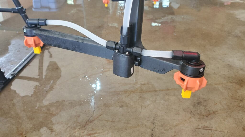
    Nozzles installed on DJI T20 drone.
    • Select the nozzle size you installed on the spray monitor.
    • Purge the air from the system.
    • Activate the spray and wait for the flow rate to stabilize on the spray monitor. This may take a few moments.
    • With the nozzles flowing, place collectors under each nozzle and collect the spray liquid for a fixed time, say one minute.
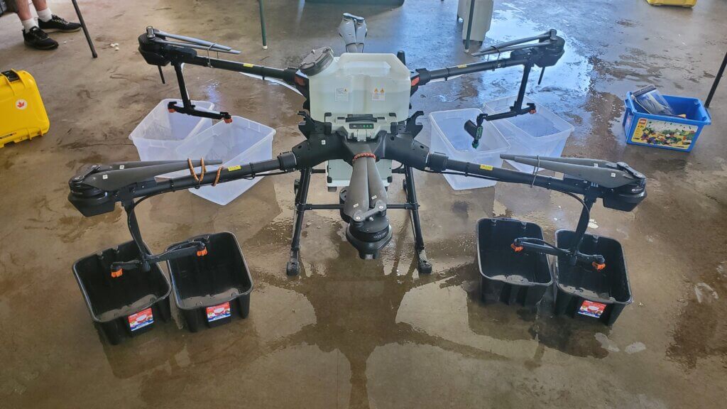
    Capturing spray during flow meter calibration.
    • Ensure the collector catches all the spray. Buckets often create turbulence. Rotary atomizers make this more difficult.
    • When the time elapses, remove the collectors and then shut off the spray.
    • Unless the shutoff is very fast and positive, leaving the collectors in place during shutoff can introduce error as the flow diminishes.
    • Confirm that the volume collected from each nozzle was identical, and that the flow rate reported by the drone flow meter is accurate.
    • Repeat to ensure consistency.
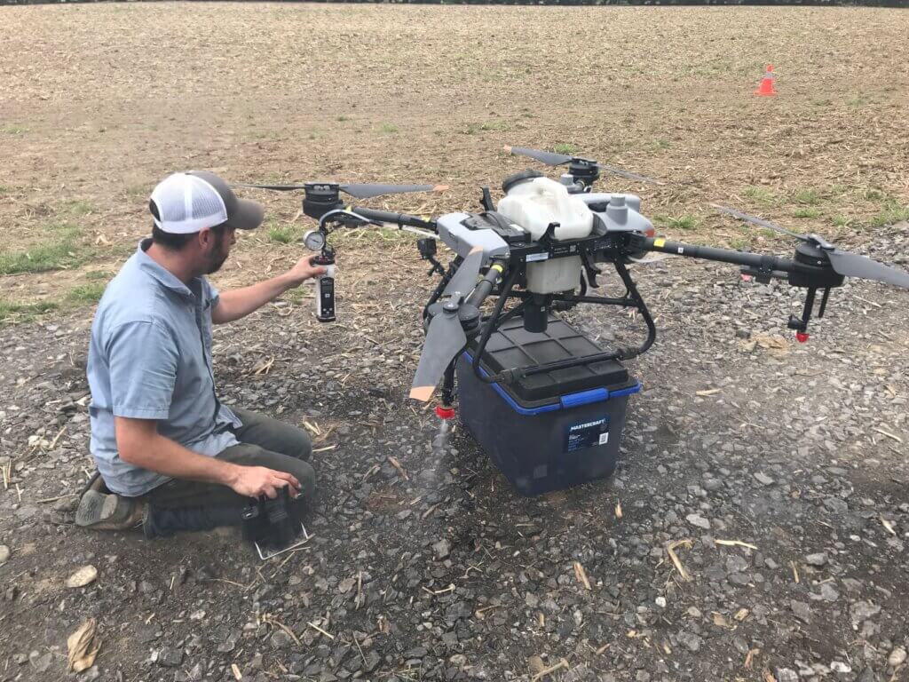
    Use of a Spot-On digital calibrating cup ensures that all spray is captured and it also reports the volume instantly.

    2. Measure the swath width

    Spray swath width is variable. For a measurement to be relevant we must evaluate spray deposition under environmental conditions that are similar to the planned spray operation, as well as use the same operational settings such as altitude, travel speed, nozzle choice, and application volume.

    Spray samplers are positioned along the ground, perpendicular to the flight path. We use water-sensitive paper (WSP) because it’s readily available, fast and easy to use, and the deposits can be analyzed visually or using simple apps that calculate coverage. We create a sampling line of WSP positioned a 1 m intervals (or maybe 0.5 m for narrow swaths). The samplers should extend to twice the expected swath width to account for any swath displacement from sidewinds.

    • Choose a day with light, consistent winds.
    • Find an open space free of obstruction in the direction of the prevailing wind.
    • Install a weather station to document conditions during flight.
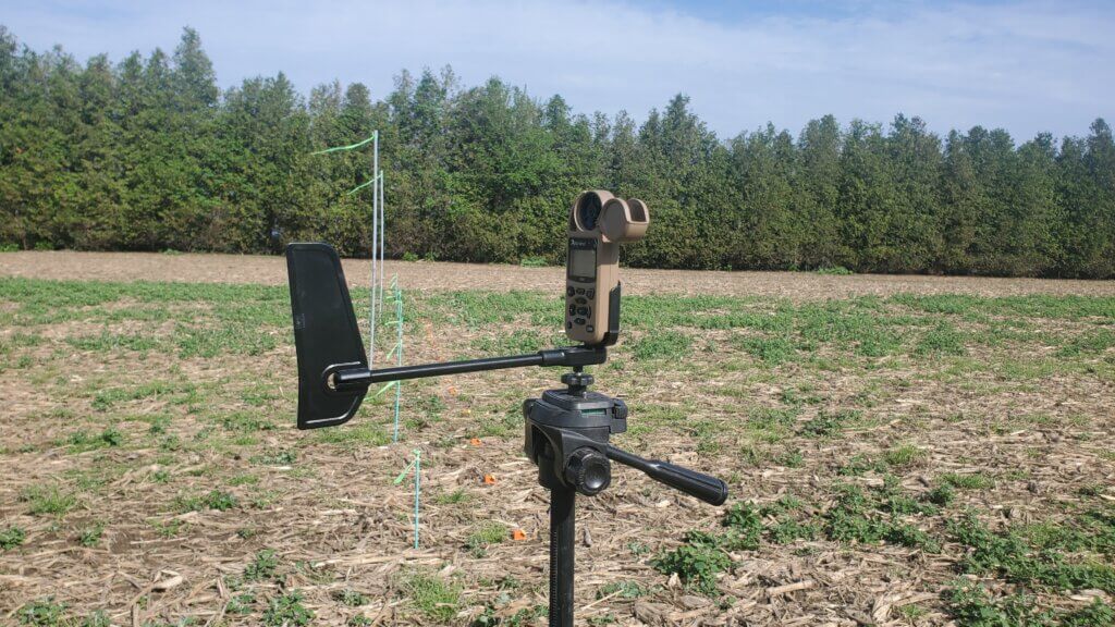
    A Kestrel 3550AG or 5550AG wind meter can record weather data and download to a phone via Bluetooth.
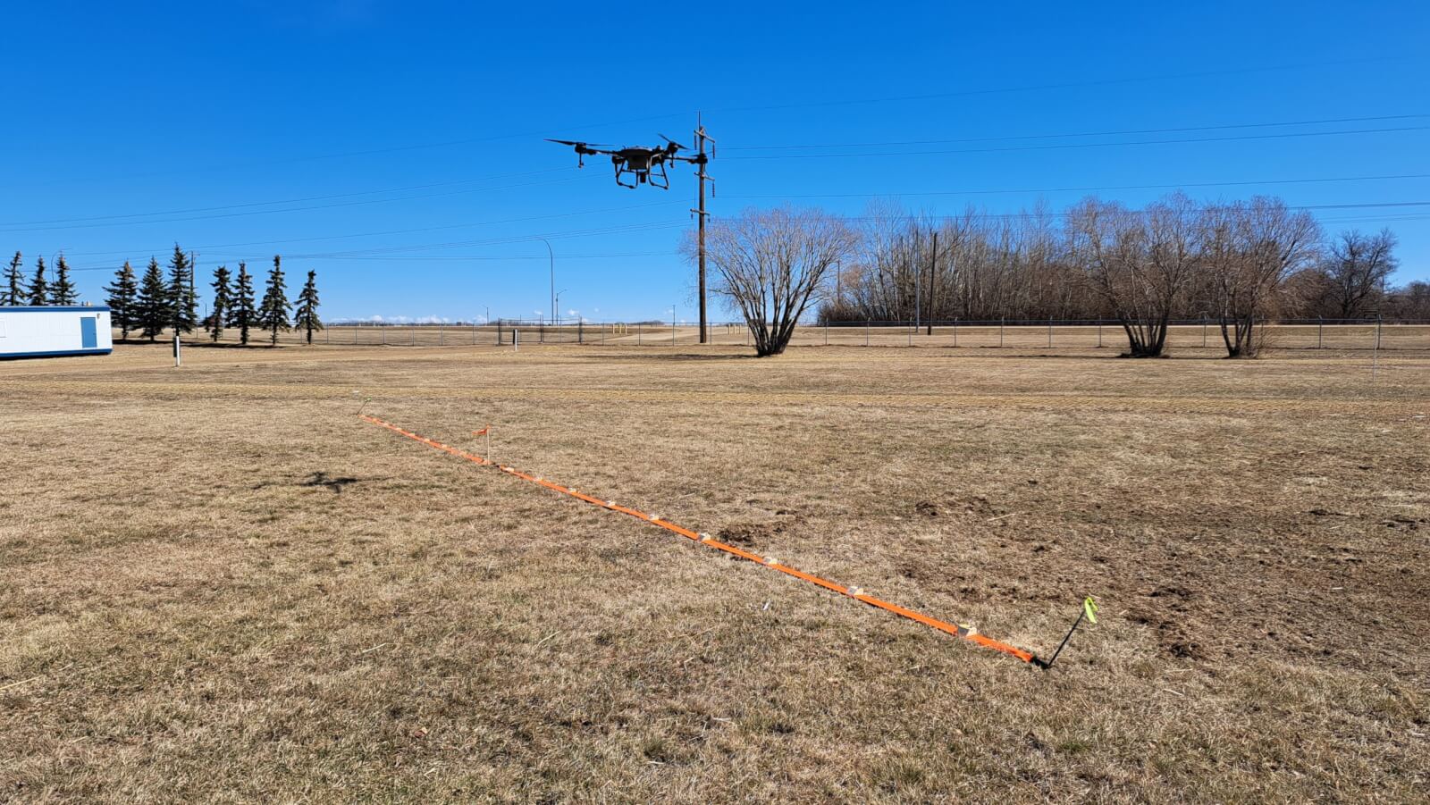
    • Mark an approximately 200 m long flight line into the prevailing wind direction by placing wire flags every 50 m.
    • At the 150 m mark, use wire flags to centre a sampler line perpendicular to the flight path. Sampler line length should be about twice the expected swath width.
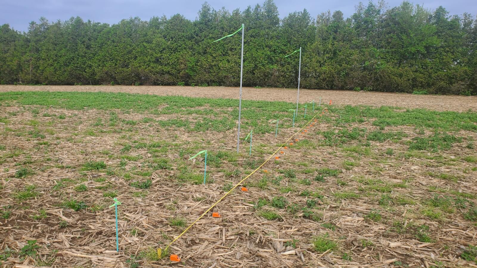
    Swath sampling line
    • Wooden blocks with paper clips can be used to secure WSP at regular intervals along the sampler line.
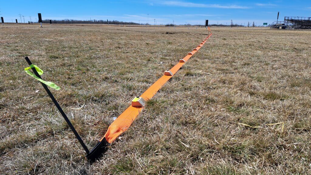
    Wooden blocks attached to a 4″ tow strap allows for easy setup and movement of sampling line.
    • Fill the drone 1/2 full.
    • Manually fly the drone along the entire flight line. The spray pressure, flow rate and altitude of the drone should be stable before it reaches the sampler line. This may take 25 meters or more depending on drone model, flight speed and drone weight.
    • Fly 50 m past the sampling line without any drone maneuvering to avoid affecting the deposit.
    • Land the drone and walk along the sampler line.
    • Note the deposits in the central region. Walk along line as the deposits taper off, looking for deposits that are approximately 50% of the average central deposits.
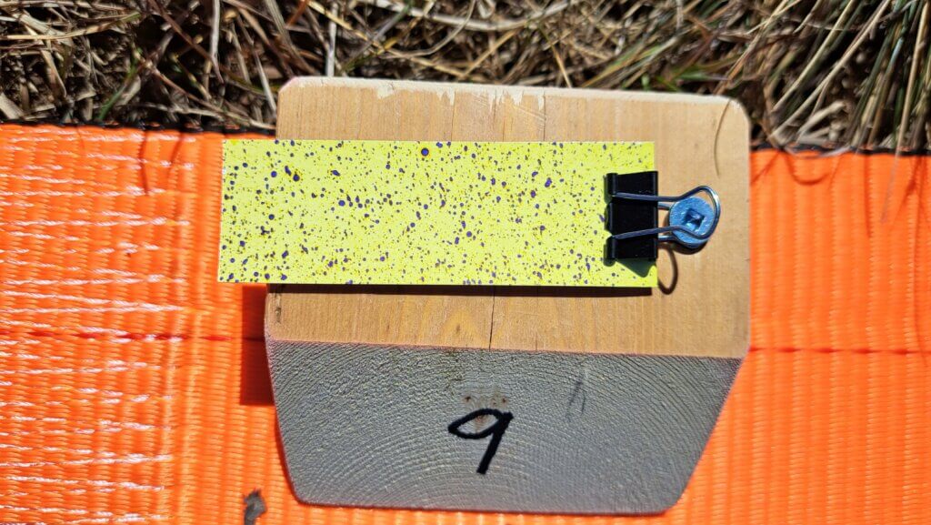
    Water-sensitive paper following a drone application.
    • Estimate the distance between these deposits on both edges of the swath. This is the estimated swath width that can be entered for the second flight.
    • Replace the WSP with a fresh set, refill the drone to 1/2 full, and repeat the flight two more times.

    Other methods perform a more advanced assessment by analyzing the entire swath, and not just intervals. These methods use dyes and dedicated hardware to quantify the deposits along strings or paper samplers.
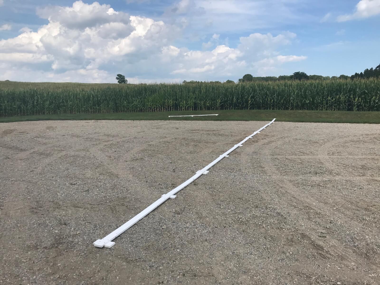
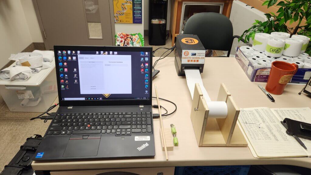
    The Swath Gobbler documents swaths at high resolution using lengths of 3″ bonded receipt paper, food grade dye, and a digital scanner.
    The Application Insight LLC Swath Gobbler scanner in action.

    3. Analyze the Pattern

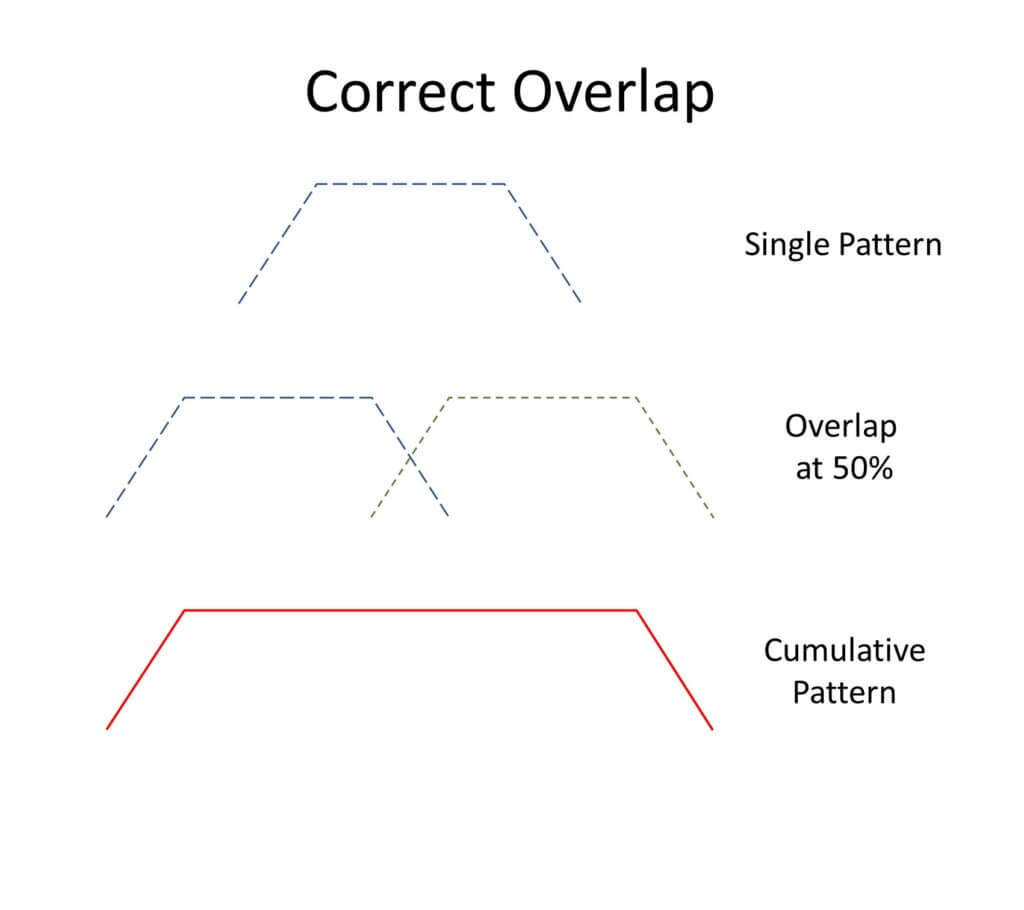
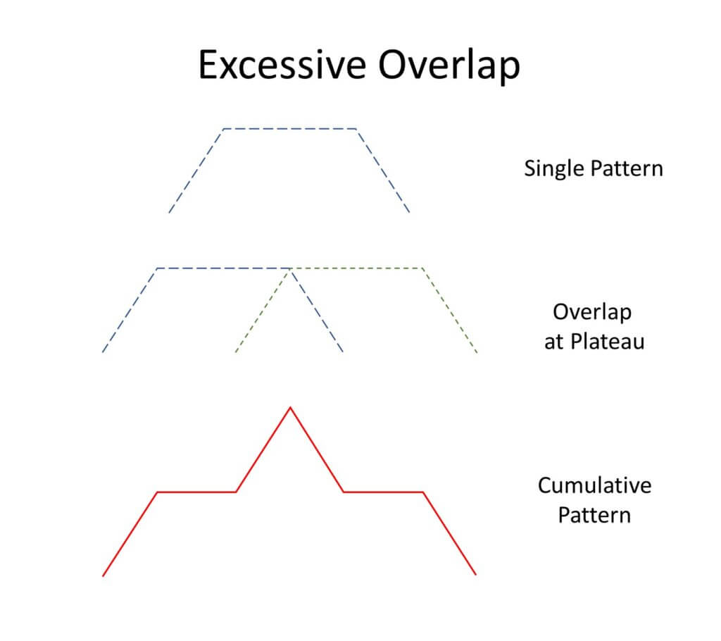
    The nearest approximation for drone swathing is that of a manned aircraft. The spray pattern of an aircraft is tapered, meaning the highest deposition is near the centre of the swath, and the edges of the swath fade to zero deposit. In order to achieve consistent coverage, we need the edges of the spray swath to overlap so the cumulative coverage at the edges is closer to that in the centre. Too little overlap leaves gaps and too much overlap results in excessive deposit.
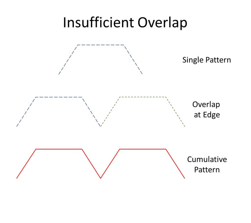
    Insufficient overlap creates gaps in coverage
    Excessive overlap results in over-dosing and waste
    Correct overlap is necessary for efficient and effective application.

    Deposits from drones can be highly variable. The challenge is to find an overlap distance that minimizes this variability, minimizes both over- and under-application, and maximizes swath width. Download a copy of an app we’ve developed to help you with this process.

    The first step is to estimate a reasonable average deposit, called “Threshold”. The app graphs the deposits from each sampler, and the user estimates a point on the Y axis (Relative Deposition) that represents the average maximum deposit. This could be the maximum value of the plateau, or a midpoint between the maximum and a nearby dip. The app assumes a value that is 90% of the maximum, to start.

    We then take 50% of this estimated average deposit, and find the two distances on the X axis (Sampler Locations) that intersect the curve at these points. The distance between these two points is our first estimate of the swath width. If two adjacent swaths are spaced so the edge of one overlaps 50% with the next, the overall cumulative deposit should be relatively even.
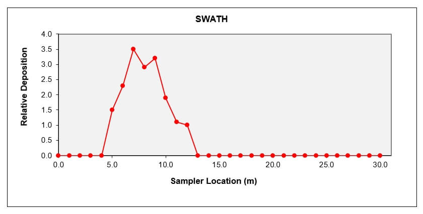
    The coverage information from each sampler location is graphed to create a deposit pattern.

    We can alter the amount of overlap to improve the apparent uniformity, but be cautious. For example, even though we can often improve the uniformity by narrowing the swath width, this can add deposit to the area under the drone and raise the overall deposit amount. That would be waste. Plus, the narrower swath also lowers the productivity of the drone. Use the app to establish a swath width that has the lowest variability (Coefficient of Variability or CV) AND results in a balance between over- and under-dosing. The app has an “Optimize” button that can do this for you.

    It’s possible to select a racetrack or a back and forth pattern. We’ve been using the racetrack pattern even though in real life the drone will frly back and forth, for the following reason: We expect a field to be sprayed in a sidewind. The tail of the deposit will always be on the same side of the pattern even with a back and forth flight path. In essence, the wwind creates a racetrack pattern for us.
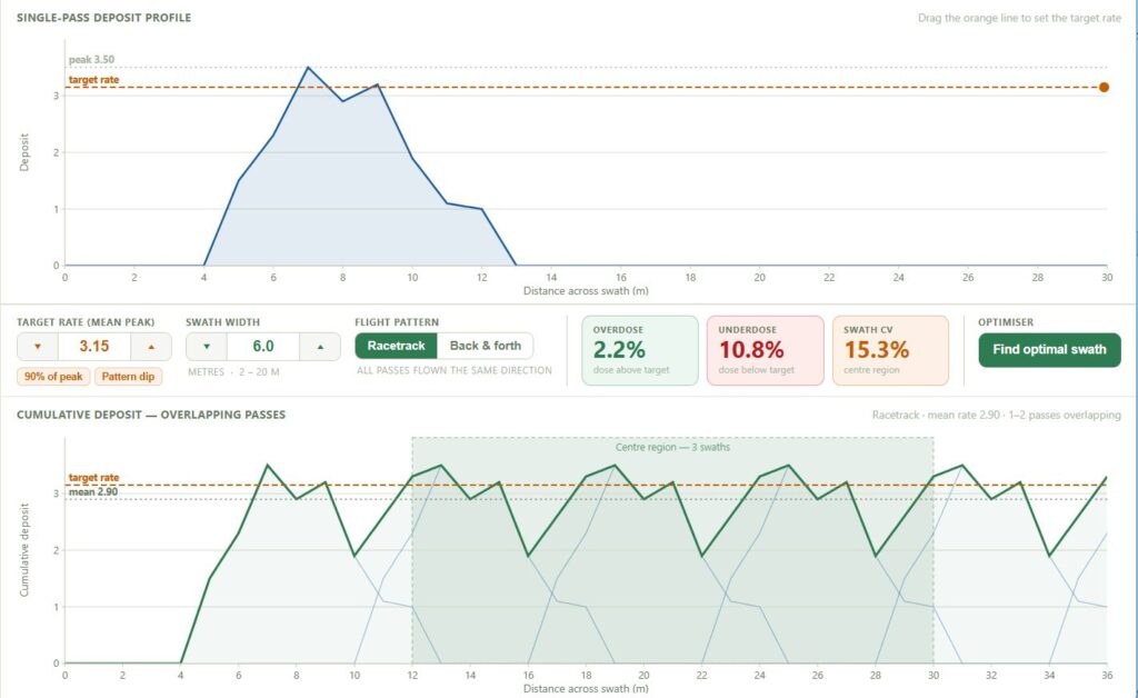
    The amount of overlap is adjusted to minimize variability (CV) and both equalize and minimize over- and under-dosing.

    The app allows you to import your data using an Excel file. If the file has multiple data column, the user can select the column to be analyzed. From that point, other columns can be selected as the analysis proceeds. Each analysis can be saved and exported as a pdf file.

    4. Recognize the factors that influence swath width

    Operational use case affects swath width

    Swath width is affected by altitude, speed, water volume and spray quality. Generally, higher altitudes, lower volumes, and finer sprays will result in a wider swath. Unfortunately, the same configuration also results in greater drift. It is recommended that swath widths be determined for each spray volume and nozzle arrangement that will be used.

    Drones will be applying low water volumes and this requires a critical assessment of coverage to ensure the deposit density is sufficient to achieve the desired result. A low volume will require a finer spray for minimum coverage to be realized. Coarser sprays that reduce drift and evaporation will need higher water volumes and result in narrower swaths. Significant time may need to be invested to understand the effects of operational settings and environmental conditions on spray deposit uniformity and swath width.

    Effective Swath Width and the Agronomic Use Case

    The relatively sparse coverage at the extremes of the measured swath width may be insufficient to elicit the desired biological result. The Effective Swath Width (ESW) represents the segment of the total swath width that results in pesticide efficacy. In some use cases, the two widths can be similar, but typically the ESW is only a fraction.

    The difference is influenced by the “Agronomic Use Case” which includes factors such as:

    • Spray mix rheology (i.e. the interaction of spray mix viscosity and atomizer design on droplet size)
    • Minimum effective dose: This is a complex relationship between coverage, spray mix concentration and pesticide mode-of-action that results in an effective result while minimizing the environmental impact.
    • Target location (e.g. a pest within a dense canopy or a weed on relatively bare ground)

    Taken collectively, research has shown a 20-30% reduction in ESW for corn, wheat and soybean fungicide applications compared to swaths measured on open ground. Conversely, herbicides sprayed on bare earth or sparse vegetation can produce an efficacious response 20% wider than the measured swath width. The impact of agronomic use case on ESW must be considered during mission planning.

    Additional pointers

    Here are a few tips and tricks to help you be successful when calibrating your drone.

    • Drone patterns will have deposit peaks and valleys in the central region. Repeated runs are needed to confirm that these are real and persistent. If so, then adjustments in flying height, spray quality, or water volume may be needed to eliminate them.
    • The absence of pressure gauges on drones can be corrected by installing an analog gauge in-line with one of the spray nozzles. If may be necessary to mount an auxiliary camera on the drone to record this gauge. We have observed strong fluctuations in spray pressure, particularly on starting a spray swath, that were not reflected in the reported flow rate.
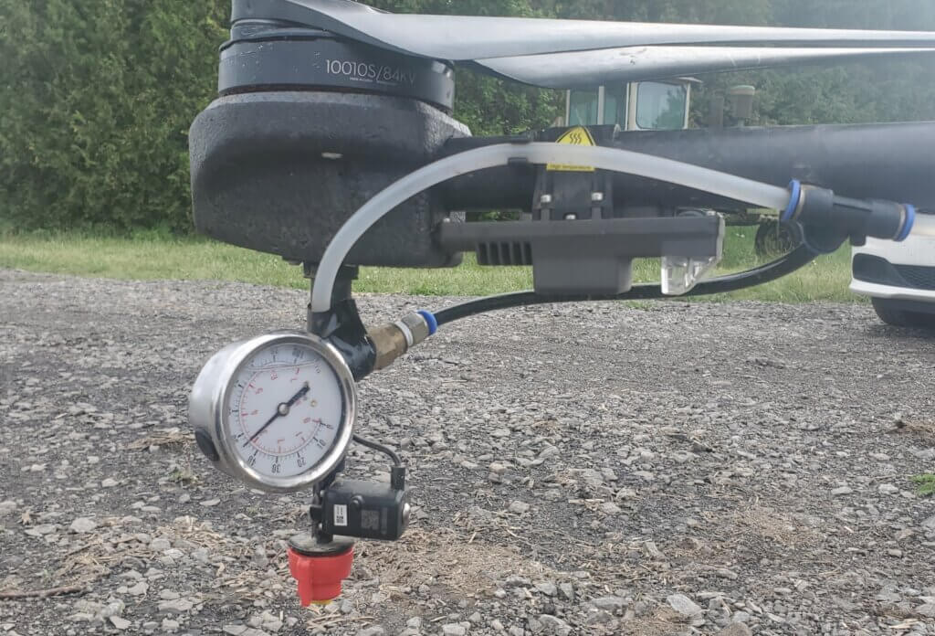
    A pressure gauge can be plumbed into a drone without affecting flight behaviour. A camera is trained on it to read pressure during a flight.
    • Many drones have the option of recording the flight screen during a mission. This will provide a record of the performance of the drone, and can be valuable should performance problems arise.
    • Although swath width calibration is done by flying into a headwind, the actual spray application should be done with a side wind. Start at the downwind edge of the field and turn into the wind. The drone is symmetrical and the tapered spray patterns should equalize the deposits. Alternately, flying into a headwind and returning with a tailwind can alter the aerodynamics of the spray deposition process, alternating between a wider and more narrow swath width, respectively.

    Drone spraying will walk a razor’s edge of sorts – there is little room for error when using scant water and fine droplets. Getting the basics right has never been more important.


  • How Much Pesticide in the Tank?

    How Much Pesticide in the Tank?

    Sprayer math can be intimidating, but the effort gives solid value. When combined with a calibrated sprayer you reap the following benefits:

    • Determine how much spray mix is required to apply the intended rate.
    • Estimate how much crop protection product must be ordered for the season.
    • Populate spray records which allow you to review practices, respond to enquiries and satisfy traceability requirements.

    There are many ways to perform sprayer math, and you need only look to local pesticide safety courses, industrial catalogues, and extension resource centres for examples. If you’re already comfortable with your current method, don’t mix and match with others. Sprayer math is a series of related calculations that employ constants to keep the units straight. It’s all or none.

    Walkthrough

    Let’s start with the classic, US Imperial formula for calculating the sprayer output. We’ll weave in Metric, later. This base formula can be adjusted to allow you to solve for any factor, as long as you’re only missing one piece of information. Turns out your high school teacher was right – you DO need algebra.

    GPM = [GPA x MPH x W] ÷ 5,940

    In this case, you can determine an output rate (GPM – gallons per minute). You’ll need to know your target volume (GPA – gallons per acre), your average travel speed (MPH – miles per hour) and your nozzle spacing (W – which is width in inches). The number “5,940” is a constant that handles all the unit conversions. If you divide the GPM by the number of nozzles on your sprayer (assuming they are all the same rate), you can hone in on the ideal nozzle size.

    But, as we noted earlier, you can do a lot more with sprayer math than just pick the ideal nozzle size. The rest of this article includes examples of both Metric and US Imperial formulae, but watch out for unit conversions. If at any time you don’t see the units you’re looking for, you can consult our unit conversion tool.

    Grab your calculator – it’s math time!

    Don’t be intimidated. With a little practice, sprayer math gets easier and it’s always worthwhile. The real trick is navigating unit conversions.

    Step 1 – How large is the area you need to spray?

    Multiply the length of the area you plan to spray times the width. If you are using metres, then divide the product by 10,000, which is the number of m2 in a hectare (ha). For feet and acres, divide by 43,560 which is the number of ft2 in an acre (ac):

    Step 2 – How much product is needed to spray the area?

    Consult the rate(s) shown on the label. In Canada, rates are often based on planted area (E.g. hectares). In Australia and New Zealand, they may be based on row length (not covered in this article). If you measure your area in acres, you’ll have to convert the rate by multiplying by a constant: 0.4.

    product-per-area

    Now multiply the area you want to spray (step 1) by the rate (step 2).

    product-per-area2

    Step 3 – How far can you go on a full tank?

    You know your sprayer output (determined through calibration) so you divide that into your tank size. Watch your units:

    full-tank-distance

    Step 4 – How much pesticide per tank? 

    Multiply the area that can be sprayed per tank (Step 3) by the pesticide rate (Step 2). Again, watch your units:

    pesticide-per-tank

    Step 5 – How much area is left to spray?

    Just subtract what you’ve already sprayed from the total area.

    area-left-to-spray

    Step 6 – How much pesticide in the last, partially-full tank?

    Multiply the area you have left to spray (Step 5) by the pesticide rate (Step 2). Yes, watch your units:

    pesticide-partially-full-tank

    Step 7 – How much spray mix will I need for the partial tank to finish spraying the total area?

    Multiply the area you have left to spray (Step 5) by the sprayer output (determined through calibration). Guess what? Watch your units:

    spray-mix-for-total-area

    Sample problems

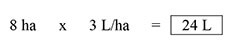
    Time to test your knowledge. Let’s suppose you want to apply a product rate of 3 L/ha to your blueberries. You calibrate your sprayer and determine your output to be 50 L/ha. Your tank holds 400 L of spray mix. Your planting is 500 m long and 200 m wide.

    Q1 – How large is the area you need to spray?

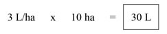
    area-to-spray

    Q2 – How much product is needed to spray the area?

    product-to-spray-the-area

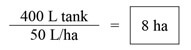
    Q3- How much area can be sprayed on one tank?

    area-on-full-tank

    Q4 – How much product should be added to a full tank?

    product-needed-full-tank

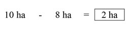
    Q5 – After the tank is empty, how much area is left to spray?

    area-left

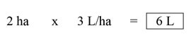
    Q6 – How much product to add to the last, partially full tank?

    product-partially-full-tank

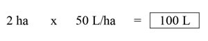
    Q7 – How much spray mix will be needed to finish spraying?

    spray-mix-to-finish-spraying

    Tank mix calculator

    You might feel we buried the lead by adding this calculator to the end of the article. It’s important for a sprayer operator to understand the math required to interpret labels and calculate tank mixes, so hopefully you read and understood the process before you got here. And now that you have, this is a very helpful tool. Try it online, or download a standalone version.

    Notable exceptions

    Certain situations aren’t covered in this article. If you are spraying a greenhouse, the math is different. If you are performing a banded application, the math is different. And, if you’re an airblast operator trying to reconcile why a pesticide label uses planted area rather than canopy volume for its rates, you’re in for some additional reading.

  • The Ultimate Sprayer Calibration and Unit Conversion Tool

    The Ultimate Sprayer Calibration and Unit Conversion Tool

    Canada, like most of the world, is officially Metric. America operates using the US Imperial system. It sounds very cut and dried, doesn’t it?

    However, anyone that’s tried to calibrate a sprayer in Canada quickly discovers that we’re really an amalgam of the two systems. We like to call it “Mock-tric“. By way of evidence, some operators still adhere to the dreaded L/ac. You know who you are. To be fair, some of our sprayers and nozzles originate from the states, meaning nozzle tables and rarely, sprayer indicators, can be in US Imperial.

    This leads to mind-bending questions such as:

    I drive 12 mph, spraying 150 L/ha and my pressure is about 40 psi. How many ml/min should my 72 nozzles emit for a product that wants a 6 oz/acre acid equivalent?

    Cue the quiet sobbing…

    Frustrated back in 2017, we created a set of conversion tables to help operators with almost any Imperial/Metric emergency. Admittedly, they were in 4-point font and therefore too cumbersome for practical use. We’ll keep one here for posterity.

    The good old days of “look-up tables”. RIP.

    Happily time has marched on and we now have a better way. Explore our new Sprayer Calibration and Unit Conversion Tool, below. While it doesn’t do it all, it certainly does a lot! You can:

    • Convert between common (and some uncommon) agriculturally-relevant units.
    • Calibrate a field sprayer for both broad acre or banded applications.
    • Calibrate an airblast sprayer for almost every traffic pattern and swath width.
    • Calibrate a plot sprayer, either for a handheld boom (any number of nozzles) or for a backpack sprayer mist/wand in 3D rows.
    • Calibrate a fogger for common closed environment structures

    To use this suite of calculators correctly, the user needs some agronomic understanding of what these variables mean and how to obtain them. In order to provide context, and reduce the friction, we’ve added a link to relevant articles at the top of each calculator.

    Grab an offline version here, or try it out below. We’ve tried to validate every path, but if you find a bug, please let us know. Once you know your calibration settings, go here to determine how much goes in the sprayer tank.

  • Determining Airblast Travel Speed – The “Air Displacements” Method

    Determining Airblast Travel Speed – The “Air Displacements” Method

    What is the “right” speed to drive when spraying?

    Airblast sprayer operators must know their average travel speed to calculate how much pesticide and time is required to complete a spray job. Note that it’s an average, not a constant, because travel speed is significantly affected by ground surface conditions (e.g. slippage), grade (e.g. hills) and the weight of the rig (e.g. as spray mix is depleted).

    The pursuit of productivity and the unchallenged status quo of traditional spray volumes, blinds many operators to the fact that travel speed is a critical factor in focusing air energy on the target canopy. As long as droplets are small enough to be entrained and directed by the air, we believe that optimizing the fit between air energy and the target canopy leads to the most frugal and effective use of spray mix and should therefore dictate travel speed. If that speed proves to be painfully slow, or terrifyingly fast, then a mismatch is revealed between the sprayer design and the operational conditions and the overall spraying strategy should be reconsidered.

    This article describes a method for modelling an ideal travel speed. It can be used as a sanity check for existing operations or for those seeking to evaluate the fit of a new airblast sprayer. However, this method can only approximate travel speed. A true optimization of sprayer settings will require fine tuning using the ribbon method and, ultimately, coverage feedback from water sensitive paper (see here and an older article here). We’ll begin with how to measure average travel speed.

    How to measure average travel speed

    Beware the tractor speedometer or rate controller that monitors wheel rotations; both can be fooled by changes in wheel size, tire wear or slippage. GPS or radar-based speed sensors are the most accurate method.

    Those that prefer a manual method can follow this classic protocol for determining average travel speed:

    1. Go to a row that is representative of the terrain in your planting. Measure out a distance of 50 m (150 ft) and mark the start and finish positions with wire marker flags.
    2. Fill the sprayer tank half full of water.
    3. Select the gear and engine speed in which you intend to spray. If using a pull-behind sprayer, ensure the PTO is running or you could introduce errors.
    4. Bring the sprayer up to speed for a running start and begin timing as the front wheel passes the first flag. This is far easier when there are two people.
    5. Stop the timer as the front wheel passes the second flag.
    6. Stay out of any ruts and run the course two more times.
    7. Determine the average drive time for the three runs (i.e. the sum of all three times in seconds divided by three).
    8. Finally, calculate travel speed using one of the following formulae, depending on preferred units:

    Ground Speed (km/h) = Average drive time for 50 m (s) ÷ 13.9 (a constant)

    Those that prefer a less accurate but convenient hack can download any smartphone speedometer app that can calculate an average (similar to a runner’s GPS wristwatch). Fill the sprayer tank half full and drive a representative section of your operation with the fan on and the spray off. Consult the phone for your average speed for each pass. Take a screen shot and email it to yourself as a time-stamped component of your spray records.

    The “Air Displacements” method

    Dwell time

    Airblast sprayers use fans to move a volume of air at a certain speed, often measured in m3/hr or ft3/min. Imagine that volume of air as a three dimensional shape extending from the air outlet over a distance. Likewise, imagine the void between the sprayer outlet and the target canopy as a three dimensional shape penetrating roughly halfway into that canopy (assuming we intend to spray every row).

    How long must the sprayer dwell in one spot before it pushes all the intervening air out of the way and replaces it with spray-laden air? If the sprayer drives too slowly, it will wastefully push spray through and beyond the target (i.e. blow-through). If the sprayer moves too quickly, the spray will not have an opportunity to penetrate the target canopy and most certainly not reach the highest point. This concept of focusing air energy using travel speed is called Dwell Time.

    We want to calculate the volume of air the sprayer generates, compare that to the volume we want displaced, and then determine how fast we must drive to optimize the fit. We can do all this with a tape measure, an anemometer, and a partner to record the data and do a little math.

    1. Measure air outlet area

    With the sprayer safely off, measure the area of the air outlet(s) on one side of the sprayer. We’ll use a Turbomist 30P Low Drift Tower (below) as an example. There are two air outlets that are 5 cm wide by 150 cm high for a total area of 0.075 m2 on each side. Be sure to look inside the outlet for any irregularities like baffles or obstructions intended to block air. Subtract those areas from the total. Don’t worry about small things like nozzle bodies.

    For rectilinear outlets: Height (m) x width (m) = Area (m2)

    For circular outlets: 3.14 x radius2 (m) = Area (m2)

    The air outlet on this Turbomist 30P Low Drift tower sprayer is 5 cm wide by 150 cm tall for a total area of 0.075 m2.

    2. Measure air speed

    First, a few safety warnings: High speed air is loud and can carry debris, so always wear ear and eye protection and respect the hazards inherent to working with air-assist sprayers. Only use an anemometer rated for at least 160 km/h (100 mph) (e.g. here). Do not use a handheld weather meter such as a Kestrel because the impellor could be destroyed and become dangerous shrapnel.

    Use an anemometer rated for at least 160 km/h (100 mph) (e.g. here). Do not use a handheld weather meter such as a Kestrel because the impellor could be destroyed and become dangerous shrapnel.

    Bring the fan up to speed and holding the meter about 25 cm (10 in.) from the outlet, measure the air speed at several locations along the air outlet both vertically and horizontally. We calculate an average speed because many air outlets do not produce uniform air speed or volume along their outlets. For this example, we measured four locations along the air outlet on both sides of the sprayer and saw significant differences. We did this both in low and high gear (see table below).

    High GearHigh GearLow GearLow Gear
    Location Along OutletLeft Side (m/s)Right Side (m/s)Left Side (m/s)Right Side (m/s)
    Top 1/441.180.342.924.6
    Upper34.932.226.430.8
    Lower30.830.024.026.4
    Bottom 1/433.540.226.831.3
    Average35.145.730.028.3
    Anemometer readings from the low drift tower sprayer outlets, on left and right side, in high and low fan gear. Four readings from bottom to top to determine the average. Readings taken 25 cm from edge of outlet and PTO set to 540 rpm.

    Multiple air outlets

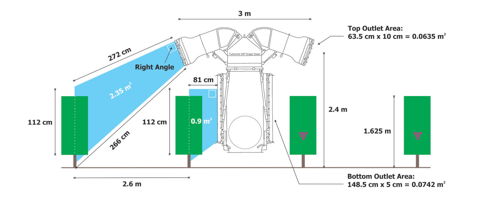
    Before we continue with the method, let’s change sprayers to this Turbomist 30P Grape Tower (below). The design is intended to spray adjacent rows from the vertical outlets (5 cm x 150 cm = 0.075 m2) along the tower. The upper, inverted outlets (10 cm x 63.5 cm = 0.0635m2) throw spray over the adjacent rows and cover the outside rows. The intention is to improve productivity by covering four rows of grape (or possibly three) per pass.

    The Turbomist 30P Grape Tower Sprayer is a multirow system intended to drive every third or fourth row.
    Lower, vertical ducts are 5 cm x 150 cm = 0.075 m2
    Upper, inverted ducts are 10 cm x 63.5 cm = 0.0635m2

    However, when we consider this design through the Air Displacement lens, it’s almost like having two sprayers performing two jobs simultaneously. The vertical outlets and the upper, inverted outlets are different shapes. Further, their position (distance and angle, as the top outlets are angled back more aggressively) relative to their respective target canopies are significantly different. How fast must this sprayer drive to optimize the fit? Do we have to compromise coverage and incur drift and waste from one set of outlets to accommodate the other set? The manufacturer has worked to address this potential issue by partitioning the majority of the air energy to the top outlets, but let’s see how that affects travel speed.

    3. Total volumetric flow

    Having already measured the outlet area, we then measured average air speed (see table below).

    High GearHigh GearLow GearLow Gear
    Location Along OutletLeft Side (m/s)Right Side (m/s)Left Side (m/s)Right Side (m/s)
    Top Outlet27.026.527.026.0
    Bottom Outlet12.013.010.512.5
    Average anemometer readings (n=4) for top and bottom outlets, on left and right side, in high and low fan gear. Readings taken 25 cm from edge of outlet and PTO set to 540 rpm.

    Now we can use these two values to determine how much air the sprayer generates by calculating total volumetric flow. We first have to convert air speed from m/s to m/h to make the units work, so just multiply it by 3,600. Then we multiply that by the outlet area and we get the table below.

    Average air speed (m/s) x 3,600 (a constant) = Average air speed (m/h)

    Average air speed (m/h) x Outlet area (m2) = Total volumetric flow (m3/h)

    High GearHigh GearLow GearLow Gear
    Location Along OutletLeft Side (m3/h)Right Side (m3/h)Left Side (m3/h)Right Side (m3/h)
    Top Outlet6,172.06,058.06,172.05,944.0
    Bottom Outlet3,240.03,510.02,835.03,375.0
    Total volumetric flow for top and bottom outlets, on left and right side, in high and low fan gear, with PTO at 540 rpm.

    4. Target volume to displace

    Now that we know the volume of air the sprayer generates, let’s determine the volume of air we need to replace with that spray laden air. This is really the only tricky bit because you have to picture a cross section and then measure the shape. See the illustration below.

    For the bottom outlet, it’s simple. The outlet is 81 cm from the grape panel and the grape panel is 112 cm high. We calculate the area of a rectangle by multiplying length by width, so:

    Length (cm) x Width (cm) = Area (cm2)

    However, the sprayer design makes the top outlet’s job trickier to figure out. This isn’t a rectangle, it’s a “quadrilateral”. We get this odd shape when either the sprayer outlet or the target canopy are significantly taller than the other. Fortunately this one has a right angle so we don’t have to brush off our high school trigonometry textbooks. Instead, we can lean on the internet using this link and plug in the values. As we can see below, the cross sectional areas spanning from the outlets and the middle of the target canopies are 0.9 m2 for the bottom outlet, and 2.35 m2 for the upper outlets.

    This gives us a cross sectional area, but we need to convert that to a volume so we can compare the air generated to the air needed. To do that, we multiply the cross sectional area by 100 m, representing how much air would be needed over 100 m of row length. The formula and the results are presented below.

    Cross sectional area (m2) x 100 m of row length = Target displacement volume (m3)

    OutletTarget Displacement Volume (m3)
    Top Outlet235.0
    Bottom Outlet90.0
    Target displacement volume for each outlet over 100 m of canopy row.

    5. Displacement rate

    We see the target displacement volumes for each outlet are significantly different. Assuming the air from the upper outlet maintains its integrity and reaches its target canopy without being blown off course, it must produce enough air energy to fill more than twice the displacement volume of the lower outlet. We can see from the earlier calculations that it does produce almost twice the total volumetric flow. But is it enough? To know we must calculate the Displacement Rate for each outlet. Let’s just focus on the left side of the sprayer in high gear.

    Total volumetric flow (m3/h) ÷ Target Volume (m3) = Displacement Rate ( displacements/h)

    OutletDisplacement Rate (displacements/h) for left side of sprayer in high gear
    Top Outlet26.25
    Bottom Outlet36.0
    Displacement rates for the outlets on the left side of the sprayer in high gear.

    So we see that the outlets at the top of the sprayer, if stationary, could displace the target volume of air 26.25 times an hour. However, the lower outlet would displace its target volume 36 times in that same hour. We see that we might have a problem. But this is for a stationary sprayer and not a sprayer in motion. The last step gives us what we came here for.

    6. Ideal travel speed

    We can now determine the ideal travel speed for this sprayer using that same 100 m row length.

    [Displacement rate (displacements/h) x 100 m of row length] ÷ 1,000 (a constant) = Ideal travel speed (km/h)

    OutletIdeal travel speed (km/h) based on left side of sprayer
    Top Outlet2.6
    Bottom Outlet3.6
    Ideal travel speed for each outlet on the left side of the sprayer in high gear.

    As we stated at the beginning of this article, this is only a model. It doesn’t account for canopy density and assumes the spray laden volume of air produced by the sprayer can reach the target intact over a given distance. However it does indicate that there is a potential issue that will lead to either over spraying the adjacent row (slower travel speed) or under spraying the distant rows (faster travel speed) which could lead to waste, drift and poor coverage.

    In the image below, we chose to drive close to 2.6 km/h in high gear. No effort was made to adjust the liquid flow (i.e. change the nozzles) so there was too much spray volume here, but we can see the losses on the left (upwind) side, and the blow-through three rows over on the right (downwind) side. Leaving aside the excessive liquid volume, we could drive faster or reduce the fan gear to reduce the blow-through on the adjacent rows, but we may go too fast (or reduce the rate of air displacement) for the upper outlets to reach the target. We can already see the integrity of the upper-left outlet breaking down as it sprays into the wind.

    Testing a travel speed. No effort was made to adjust liquid flow, which is excessive here. Cross wind was from the left to the right in the image. Photo by Corey Parker (Instagram: _parkerproductions)

    Take home

    An ideal travel speed for an airblast sprayer is more than just being productive. The spray must reach and penetrate the target. If this requires dangerously high speeds, or if you simply can’t move slowly enough, it suggests a problem with the spraying strategy. Changes will have to be made to the sprayer, the target canopy, or even the weather conditions you’re willing to spray in. Getting the job done quickly should not compromise the quality of the job. Use this method to re-evaluate your practices, or to assess the capabilities of candidate sprayers if you’re considering a new purchase. Be sure to confirm what this model is telling you using some coverage indicator, such as water sensitive paper.

    Calculator

    Now that you’ve read through the process, you can try this online calculator designed to make the process a little easier. The embedded illustrations are there for general guidance, and may not reflect the sprayer design, but the calculations work. Recognize that while this calculator will provide an idealized travel speed based on the data entered, it cannot judge whether the outcome is realistic. Obviously a recommendation to drive 25 km/h is unrealistic, but it does alert the user to the fact that the sprayer is overpowered. Try it out!

    Dr. David Manktelow, Applied Research and Technologies Ltd., is gratefully acknowledged for patiently explaining the concept of “Air Displacements” to the author.

  • Airblast Nozzles – Distributing Flow

    Airblast Nozzles – Distributing Flow

    There’s a certain deer-in-headlights expression that creeps onto a sprayer operator’s face when we discuss nozzle selection. We sympathize with our field sprayer clients given the variety of brands, styles, flow rates and spray qualities they must choose from. And PWM has made the process even more complex. However, airblast operators face an additional challenge; Unlike horizontal booms, vertical booms often distribute the flow unevenly to reflect relative differences in the distance-to-target and the density of the corresponding portion of target canopy. We discuss the broader, iterative process of nozzling an airblast boom here, but in this article we focus on the topic of flow distribution.

    An overwhelmed operator trying to nozzle a boom.

    The question of “which rate goes where” is still debated. It’s led to diagnostic devices called Vertical Patternators which show the profile of the spray. Operators can use these to visualize their distribution… but they are few and far between. For the rest of us, deciding on the best distribution begins with understanding how the practice evolved.

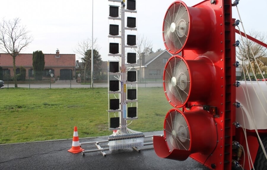
    The AAMS vertical patternator. The mast moves back and forth across the swath of a parked sprayer. Each black collector intercepts the spray at different heights. The fractions collect in the tubes at the bottom to show relative volume.
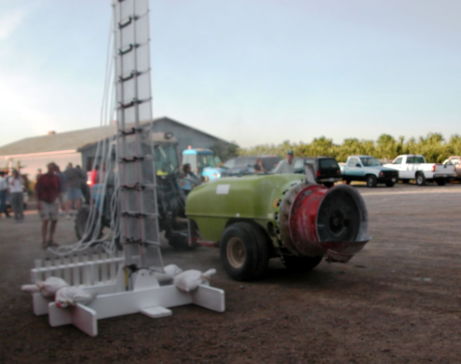
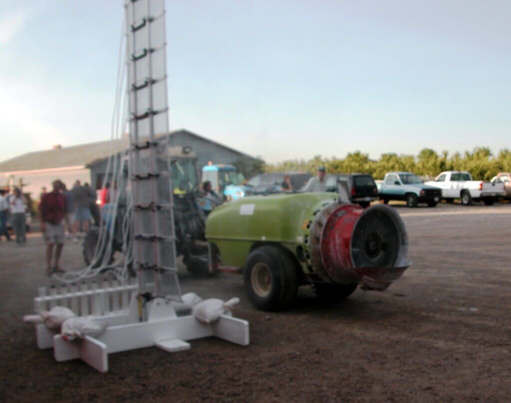
    A blurry shot of an OMAFA-built vertical patternator. The sprayer parks in front of the screens, which intercept spray. It’s collected in troughs and runs into columns that show relative volume.

    1950s

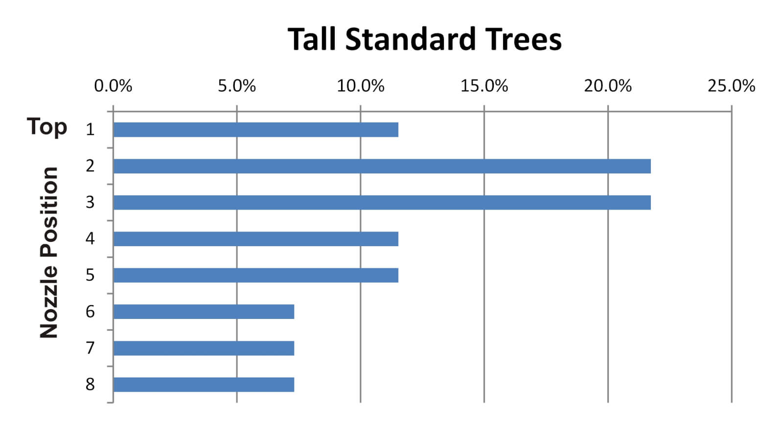
    In the 1950s, the mantra was to blow as much as you could, as hard as you could, and hope something stuck. At the time, John Bean promoted a method called “The 70% Rule” whereby operators used full-cone, high volume disc-core nozzles to emit the vast majority of the spray from the top boom positions. John Bean provided a slide-rule calculator to help operators configure booms to align the top nozzles with the deepest, densest portion of the 20-25 foot standard trees they were trying to protect. Back then, most airblast sprayers were engine-driven low-profile radial monsters capable of blowing to the tops of those trees. The practice persisted into the 60s and was encouraged by Cornell University (Brann, J.L. Jr. 1965. Factors affecting the thoroughness of spray application. N.Y. State. Arg. Exp. Sta. J. paper no. 1429).

    The profile of the spray would have looked something like the following graph:

    1970s

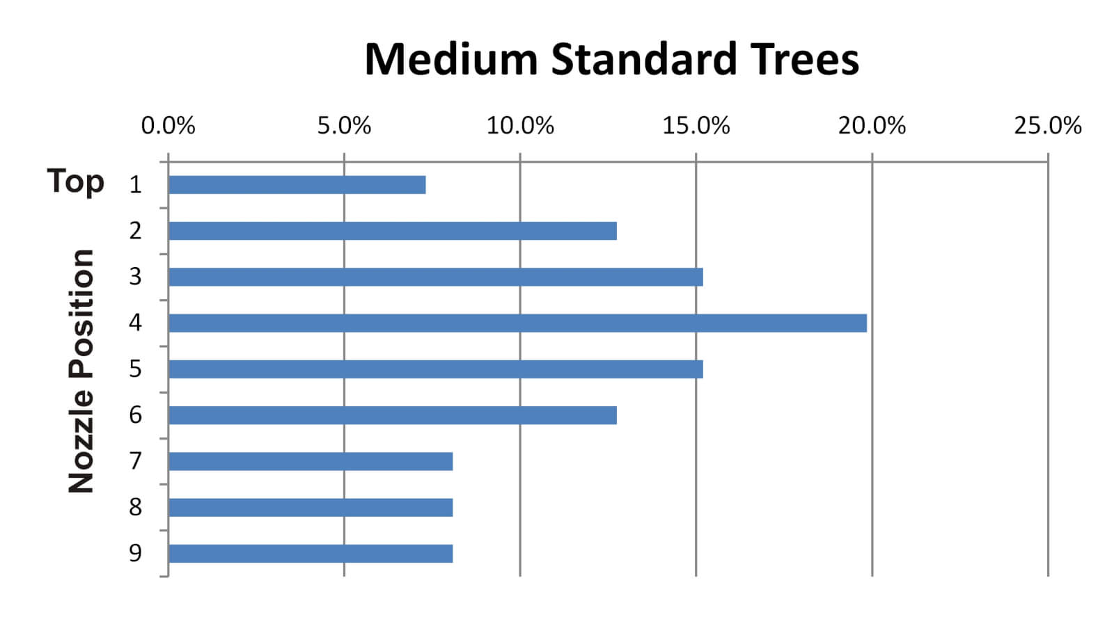
    In the 70s, extension specialists began advising operators to tailor the distribution to match the orchard spacing, tree architecture, canopy density and weather conditions. we reached deep into our archives for the Ontario Ministry of Agriculture and Food’s 1976 publication entitled “Orchard Sprayers” to see what we used to tell airblast operators.

    The 1976 update of Ontario’s 1971 “Orchard Sprayers” guide. A trove of hard-earned knowledge that still has relevance today. I love that the Minister’s name, and not the author’s, is on the cover. Let’s set the record straight: R. W. Fisher, D. R. Menzies and A. Hikichi, based in Vineland and Simcoe, Ontario.

    Here’s a synopsis of what was advised:

    1. Choose a tree size and shape that is typical of your orchard and park the sprayer at the normal spraying distance from it.
    2. Find one or two middle nozzle position(s) and air deflector or vane settings that direct the spray up through the top-inside of the tree. This is called the “middle volume zone”.
    3. Find rates that will give a large output in this middle volume zone, and smaller outputs for positions above and below.
    4. The total output must still add up to the target volume.

    It seemed operators were getting away from high rates in the top positions and instead shifting the distribution to match the canopy shape and density. If we were to follow these recommendations, the spray profile would look something like this:

    Later, Agriculture Canada’s 1977 publication entitled “Air-Blast Orchard Sprayers – A Operation and Maintenance Manual” had similar advice. Here we find the “2/3 boom rule” as the authors state: “To ensure good distribution through the trees, about two-thirds of the spray should be emitted from the upper half of the manifold.”

    1980s

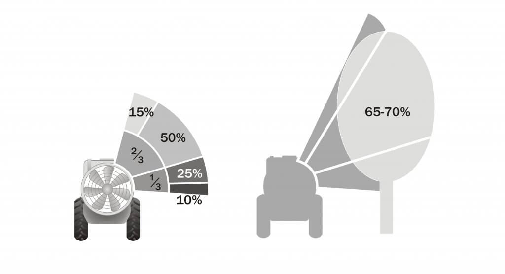
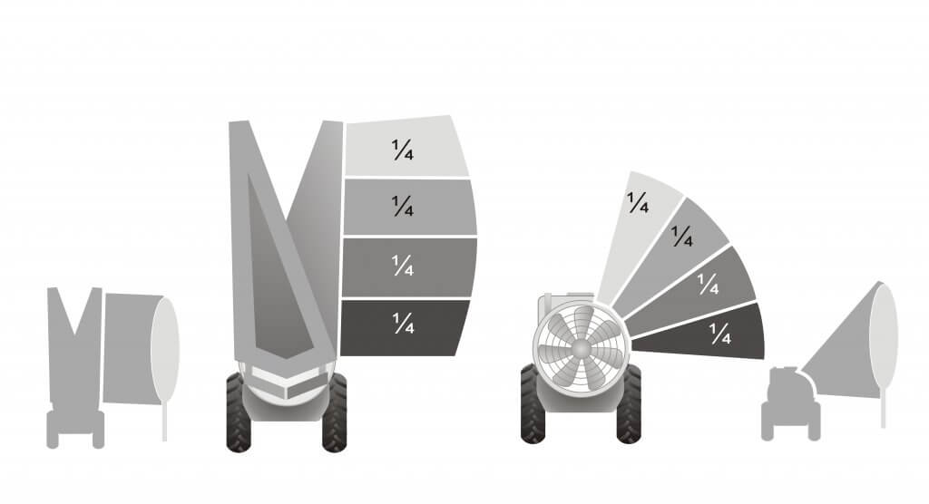
    Operators followed this approach well into the 80s, as they endeavored to aim the majority of the spray into the densest part of the canopy. Many can relate to the following illustration that divides the boom, which I modified from an array of period factsheets. The fractions represent the portion of the available boom. The percentages indicate the relative volume. Of course, it matters how large and how far away the target is for either the 2/3-boom or 70% rule to make sense (the middle volume zone is shown receiving 65-70% in the silhouette).

    1990s-2000s

    The 2/3 or 70% rules still work for standard nut and citrus trees, and perhaps for large cherry trees, but pome and tender fruit orchard architecture is densifying at this point in time. In the 90s and 00s we started transitioning from semi-dwarf into trellised, high density orchards.

    Leaping to 2005, Ohio’s Dr. Heping Zhu et al., found that a high density orchard is effectively sprayed by the same rate in each nozzle position. They wrote: “[Historical] recommendations are to use a larger nozzle at the top of each side, with the capacity of the top nozzle at least three times greater than other individual nozzles. However, results in this study with three different spray techniques showed that spray deposit was uniform across the tree canopy from top to bottom with the equal capacity nozzles on the air blast sprayer.”

    What a pleasant surprise to simplify our lives! If we can use an even distribution for dense, nearby trees, it follows that any vertical crop with the same width and density located close to the sprayer (e.g. cane fruit, trellised vines, etc.) would benefit from even distribution:

    Today (2020s)

    So, how do we do it today? There is still no simple answer; Conditions change, not all sprayers are the same, and not all applications have the same target. Let’s build on what history has taught us and establish a process to achieve better coverage uniformity and reduce waste.

    No matter the crop, the operator must first adjust air settings. Air volume and direction play the most critical role in transporting a droplet to (and into) a target canopy. Too high an air speed will cause spray to blow through the target, rather than allowing it to deposit within. Aim the air just over, and just under, the average canopy. Ensure there’s enough air to overcome ambient wind and to push the spray just past the middle of the target canopy.

    It should be noted that we assume the operator is spraying every row. With certain exceptions, alternate row middle spraying is not generally recommended. Not only can it compromise coverage on the far side of the target, it makes it far harder to match the nozzling on a single-row sprayer and is a sure-fire way to increase drift.

    Next, determine which nozzles are not needed (e.g. spraying the ground or excessively higher than the top of the canopy). Remember: hollow cones overlap very close to the boom and spread as much as 80°. Airblast sprayers rarely if ever need the lowest positions and unless spraying overhead trellises they may not need the highest either. Turning off the highest, and most drift-prone, nozzle positions in high density orchards is illustrated in the logo I was asked to create for Washington’s short-lived Pound the Plume awareness campaign in 2017.

    Then, finally, we decide on distribution. If the crop is nearby and relatively narrow, you can try even distribution. If you elect to distribute the spray unevenly to better match the variable-width target, or compensate for distance, aim half the overall output at the densest part of the canopy (the middle volume zone). Consider how the following factors might influence your choices:

    1. High humidity means more spray will reach the target, and vice versa. This is because all droplets are prone to evaporation. We have heard it said in hot, dry conditions (described by Delta T), a droplet can lose ½ its diameter every 10 feet. As they evaporate they get lighter, meaning they are less subject to their original vector and the pull of gravity, and more subject to deflection by wind. The use or coarser droplets, and/or humectants, can help, but higher volumes can help too – they increase the odds of some droplets hitting the target and actually humidify the air to slow evaporation.
    2. Windspeed increases with elevation, so spray is most likely to deflect at the top of canopies where they have already lost size (and momentum and direction). Early in the season when there is little if any foliage, wind speeds are higher overall. This is why we advise adjusting air settings using a ribbon test before considering boom distribution – you need enough air volume, aimed correctly, to get the spray to the top.
    3. The denser and deeper a canopy, the more spray is filtered and unavailable for coverage. This is why you will always achieve more coverage on the adjacent, outer portion of a canopy versus the interior. In semi dwarf apple orchards we have seen the coverage drop by half for every meter of canopy. Finer spray can penetrate more deeply because there are more droplets and they move erratically, whereas coarser droplets move in straight lines and impact on the first thing they encounter. Higher volumes will improve penetration and overall coverage, but there is a diminishing return and runoff will occur more quickly leading to more waste.
    4. Further to the last point, remember that it’s the air that propels the spray, not the pressure. Higher liquid pressure can propel coarser droplets further, but has little effect on finer droplets. imagine throwing a golf ball and a ping pong ball into a light headwind and envision how they fly. Plus, the higher the pressure, the finer the mean droplet diameter.

    Confirm Your Work

    To know how all these factors play out, you must use water sensitive paper (or some other form of coverage indicator) to diagnose the results. Remember, the goal is uniform coverage and for most foliar products, we want to achieve a minimum coverage threshold of 10-15% and a droplet density of 85 deposits per cm2 on at least 80% of the targets.

    Taking the time to match your output to the target has the potential to greatly improve coverage and reduce waste. Nozzle body flips and quick-change nozzle caps make the process of switching nozzles between blocks fast and easy. It’s worth it.

    Grateful thanks to Mark Ledebuhr, Gail Amos and Heping Zhu who edited, corrected and contributed to this article.