For those on the fly, hit play to hear a shortened, narrated version.
I have far too many photos and videos of airblast sprayers blowing straight up through treetops, or downwind through the last row, during spring applications. I chose not to include any in this article to avoid people recognizing the operations. If you haven’t seen anyone doing it, maybe it’s you!
I recognize that it can be a tricky balance to adjust a sprayer for spring applications. It’s counterintuitive, but a bare tree can be difficult to spray. Young and/or bare trees represent small targets which have a very low catch efficiency, so a lot of spray will miss. Switching nozzles to adjust rates doesn’t help much in this regard – it’s far better to adjust travel speed and air settings, and we’ll get to that in a moment.
That lack of foliage also means wind moves through the orchard unabated, so the sprayer may have to blow a little harder into the wind to compensate. In the case of a low-profile axial sprayer, which blows laterally and upward, that means creating greater risk for blowing too high, and blowing through downwind rows.
That off-target deposition represents a huge loss of materials and potential for drift incidents. To add insult to injury, many of those early season applications often have oil components, which require a drench (higher volume) and are more easily seen by bystanders (opaque droplets). All in all, it’s a bad time of year for crop protection PR. Learn more about drift and drift prevention here: BeDriftAware.
Air Adjustments
So, let’s start with air. Air carries spray droplets, so perform a ribbon test to ensure the air outlets are oriented correctly. This is achieved by adjusting deflectors (e.g. low-profile axial), the air outlets on a tower, or the entire head on a wrap-around design with individual fan/nozzle combinations.
Spray height should always exceed the canopy height by a small degree. This compensates for the increase in wind speed with elevation, the potential loss of spray height with faster travel speeds, and uneven alleys that cause the sprayer to rock, which changes the spray angle.
It is less critical that spray align with the lower portion of the canopy. As air energy wanes, or as droplets begin to lose momentum, finer droplets will slowly fall, depositing on random surfaces. Coarser droplets will quickly fall towards the bottom of the canopy, settling primarily on upward-facing surfaces. This secondary deposition can also occur from the cumulative impact of blow-through from upwind rows.
Nozzle Adjustments
Now pay particular attention to which nozzles are on or off. Park the sprayer in an alley. Stand behind the sprayer and extrapolate a direct line from each nozzle to target canopy. Nozzles that point at the canopy should be left on. Nozzles that point above or below can be blocked, or turned off, via valves or rotating roll-overs.
Some roll-over nozzle bodies can be swiveled up or down 15 degrees to fine tune the spray angle. An alternative would be to permanently rotate the nozzle body fitting in the boom line. When aiming nozzles using a roll-over nozzle body, be careful not to swivel them too far or the valve will partially close and compromise the spray pattern.
When extrapolating, remember that the centre of a nozzle only indicates the centre of the spray pattern. Cone and fan angles can span 60 to 110 degrees, depending on the influence of air. Therefore, even though the centre of the lower-most nozzle intersects the bottom of the target canopy, you may still be able to turn it off because the nozzle above has that portion covered.
Travel Speed, Wind, and Coverage Assessment
Now let’s consider travel speed. If the wind is blowing hard through the orchard, you can increase the air speed or slow down the sprayer to focus longer. However, in both cases, you run the risk of overblowing the downwind rows by a considerable margin. Easily three rows in a high-density orchard.
This downwind coverage is cumulative, so when you assess your coverage (preferably using water sensitive paper), don’t do so until you’ve made a few upwind passes. So much of that spray ends up on the orchard floor, and still more evaporates or blows up, but some of it will hit and it adds up.
Downwind Boundary
Finally, pay attention to where you are in the block. It may be necessary to turn off the downwind bank of nozzles on the final downwind three (or more) rows. That means you’ll be performing the dreaded alternate row (one-sided) application, and I’ll be the first to say that’s not ideal. However, in this case, the spray will blow back and help cover the unsprayed side. Again, use water sensitive paper to confirm the job you’re doing.
Final Thoughts
And, of course, seriously consider when it’s time to wait for better conditions. No one likes to do that, especially when rain is imminent and the ground stays soft, but the alternative is a lot of waste and a poor application. If this always seems to be the fight you’re having, maybe it’s time to consider the return on investment of a tower sprayer, or a shrouded sprayer. Towers improve matters since they more easily reach the treetop without having to blow as hard, and without angling air upward. Shrouded recycling-style sprayers (if they fit the architecture) help even more.
Plan to do all of this (especially the capital investment number crunching) before the season starts and be prepared to change sprayer settings on the fly, as required. Don’t be the subject of my next spring drift photo.
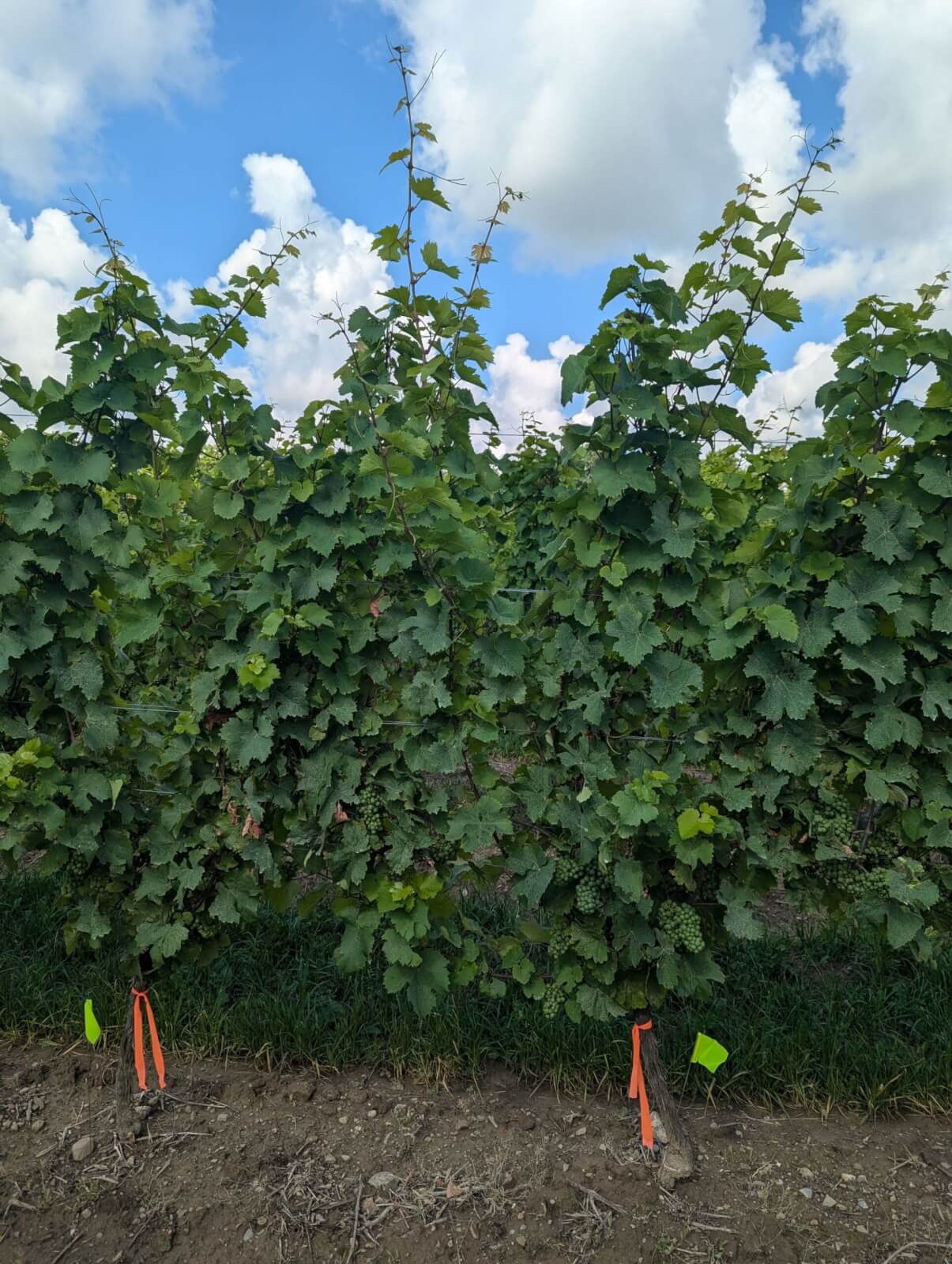
In the summer of 2024, six Ontario vineyards participated in an authorized herbicide trial. The objective was to assess efficacy as well as determine if the product fit the timing for seasonal weed and sucker management. If successful, it could replace the expensive and time-consuming manual labour required to remove suckers.
Each vineyard applied the same rate, at similar times, employing optimal sprayer settings. A few weeks after application, the researchers and registrant toured the vineyards. They were pleased with how quickly and effectively the product worked on both targets at all six locations. However, one vineyard reported visual injury on a sloped region of their operation.
This raised two questions:
Assuming the cause was drift, and not direct overspray, why did it only happen in a specific region of a single vineyard?
Whether drift or overspray, what is the potential for the applied rate to cause injury?
The vineyard manager and sprayer operator investigated the application equipment and found no problems with how the sprayer was calibrated or operated. Further, the nearby weather stations recorded reasonable environmental conditions. So, that seemed to discount accidental overspray and wind-borne drift.
Then we considered the topography. The level portion of the vineyard appeared undamaged, but as it began to slope downhill, we saw damage on leaves and shoots in the bottom half of the canopy. It was almost as if a stratum of herbicide stayed level as the ground fell away. We discussed temperature inversions, volatility, and sprayer wake, but nothing fit.
Then we stepped back and found ourselves looking up at the Niagara Escarpment. The Escarpment is a long cliff formed by erosion, separating the higher, level ground from where we stood below. And then we had an idea: Could the product have been lifted into contact with the canopy by a Katabatic wind?
The theory
On clear nights with calm winds, the ground cools rapidly. Air in contact with the colder ground cools by conducting heat to the ground and by radiating upwards. When this cooling process occurs along mountain slopes, or on top of a plateau, the cooling air becomes colder and denser, causing it flow downslope like water. Perhaps a layer of relatively cool Katabatic wind off the escarpment slid under the warmer layer of air in the downslope portion of the vineyard. And, perhaps, any product still suspended in the air was lifted upwards into contact with the grape canopy.
Cold air (blue) slides under a warmer layer of air (orange) that carries traces of herbicide in the form of Very Fine, suspended droplets. It is lifted into contact with the lower portions of the grape panels.
Even the coarsest hydraulic nozzle produces a population of driftable fines. These fines take a long time to fall, and some are essentially buoyant. In the following histograms, we see actual data from a nozzle rated between Medium and Coarse. The operators actually used an air-induction nozzle with a much coarser spray quality, but we’re using this data set as a worst-case scenario example. If we divide the volume produced into its constituent droplet sizes, we see that most of the volume is comprised of droplets between 150 and 250 microns.
However, droplet diameter shares a cubic relationship with volume. If we plot that same volume by number of droplets, we see the majority are between 18 and 74 microns in diameter. These very small droplets would fall so slowly that any atmospheric disturbance would displace them. Depending on the crop’s sensitivity to the herbicide, they might carry sufficient active ingredient to cause injury, assuming they didn’t evaporate to the point that they were no longer biologically active.
There are a lot of assumptions in this theory, and perhaps it’s far fetched, but it was the best we could figure. So, if those droplets were lifted into contact with the canopy, were they capable of causing injury? To find out, we conducted a simple, non-replicated bioassay.
The bioassay
On the morning of July 12, we filled a spray bottle with 50% of the field-rate (including 1% v/v MSO) and set the nozzle to the finest setting. We applied a single spritz about mid-way up the canopy of the same Riesling grapes on a VSP flat cane training system. We did this on the upwind side on both older (lower canopy) and newer growth (upper canopy). Then we performed a series of serial dilutions, halving the concentration each time, and repeating the application.
Our hope was to see a subtle response curve when we plotted concentration against tissue damage. Perhaps we’d even see a different curve for older versus newer tissue.
The vineyard manager photographed and recorded observations on an approximately weekly schedule, with a gap in observations between weeks three and six. The following images show the results of a ½ dose treatment, and a 1/16 dose treatment tracked during that period.
The results
We observed the following:
Fruit, foliage, and shoots were injured at all doses by three days after application.
Initial injury remained stable; no secondary injury was observed.
The degree of injury at the lowest dose was significantly more severe than the injury observed following the original May 31st application.
Regular vineyard operations, such as mechanical leaf removal in the fruiting zone and hedging, removed some of the damaged leaves and shoots.
The study did not include an assessment of harvest quality.
This was severe injury, even at the lowest rate. When compared to another herbicide commonly used for perennial weed control (e.g. Ignite SN – glufosinate ammonium) the injury we saw manifested very quickly.
Recently, researchers at Cornell have been exploring the herbicide we used in this study in perennial weed and sucker control in apple orchards. They did not experience any drift issues and found it to be effective between 90-180 ml/ha (0.5-1 oz/ac) (personal communication). That’s ~4x less than the rate proposed for registration in Canada, and it suggests the herbicide in question was certainly capable of causing the damage at very low concentrations.
Ultimately, we can’t be certain how the initial off-target damage occurred, but we were able to evaluate damage potential using a rough-and-simple bioassay that any grower can try. In unusual cases of drift it’s important to know if the product we suspect is even capable of causing the damage. A simple evaluation using serial dilution and a squirt bottle can tell us if we need to look more closely, or look somewhere else to explain injury.
Thanks to Kristen Obeid, OMAFA Weed Specialist (Horticulture) and Josh Aitken, Vineyard Manager of Cave Spring Vineyard for their contributions to this work.
This work was performed with Mark Ledebuhr (Application Insight LLC.), Adrian Rivard (Drone Spray Canada) and Adam Pfeffer (Bayer Crop Science – funding partner). Amy Shi is gratefully acknowledged for her assistance with statistical analysis.
Introduction
In June 2017, Transport Canada cleared the general use of drones. In 2018, Health Canada clarified that the use of Remote Piloted Aircraft Systems (RPAS) for pesticide application is not permitted under the Pest Control Products Act without sufficient data to characterize any associated risk. Currently, there are no liquid pest control products registered for application by drone in Canada.
Stakeholders want to use drones to apply pest control products in Canada. To that end, several research trials have been approved by Health Canada. However, multi-rotor drones represent a unique application technology more akin to air-assisted ground sprayers than manned aircraft. As such, conventional models for drift, exposure and efficacy may not apply. Fundamental questions surrounding the utility of drones must be addressed before efficacy and residue can be considered in any relevant context.
Research and user experience has identified, and is beginning to understand the relative influence of, external factors such as crop morphology, planting architecture, topography, and environmental conditions. Considered with the product mode of action, these factors inform operational settings such as altitude, travel speed, nozzle choice, and application volume to optimize applications. This collective “Use Case” depends on drone design, which is highly variable and rapidly evolving.
Having performed preliminary work characterizing effective swath width, and recognizing its popularity in North America, we used DJI’s Agras T10 in this study. Our objective was to evaluate fungicide efficacy on Northern Corn Leaf Blight, Tar Spot, Grey Spot and Common Rust in field corn, as applied using the T10. Drift and coverage would be characterized to provide context for the efficacy analysis, but also to develop data to inform best practices and possibly regulatory decisions surrounding risk. Aspects of the study would be repeated using conventional ground sprayer technologies to form a basis for comparison.
Objectives
Quantify spray coverage in field corn at three canopy depths, on adaxial and abaxial surfaces, as recovered tracer dye (indexed to % of applied rate ac-1), area covered (%) and deposit density (deposits cm-2).
Quantify drift as recovered tracer dye (indexed to % applied rate ac-1) collected using the horizontal flux method up to eight meters high on the immediate downwind edge of the application.
Evaluate the fungicide efficacy, applied using the T10, at 2 and 5 gpa as compared to a conventional overhead broadcast treatment at 16.7 gpa.
Material and Methods
Design
Trials were conducted between July and August of 2022 in three Ontario corn fields. The locations, the application methods and data collected are detailed in Table 1.
Field
Location
Corn Variety
Application Method
Rate (gpa)
Data Collected
1
Jaffa (42°45’56.6″N 81°02’06.5″W)
DKC45-65RIB
Agras T10
2 and 5
Drift, Coverage, Efficacy
Overhead Broadcast
16.7
Coverage, Efficacy
2
Fingal (42°42’17.9″N 81°15’15.3″W)
DKC49-09RIB
Agras T10
2 and 5
Drift, Coverage, Efficacy
Overhead Broadcast
16.7
Efficacy
3
Port Rowan (42°35’53.6″N 80°30’43.2″W)
P0720AM
Directed (Drop hoses)
20
Coverage
Table 1 – Trial sites by application method and data collected
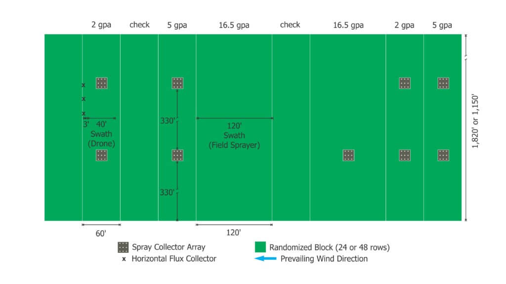
Treatments were arranged in a randomized complete block design (Figure 1). Corn was planted on 30″ centres, with about 6” in-row spacing between stalks. We targeted spray for the R1 stage of development (approx. 8’ high). Fields 1 and 2 each hosted two replicated treatments of 2 gpa, 5 gpa, and 16.7 gpa, as well as two unsprayed checks. In field 1, blocks were 60’ (24 rows) wide by 1,150’ long for the T10, and 120’ (48 rows wide) by 1,150’ long for the broadcast field sprayers. A single, 120’ swath was applied using the field sprayers, and four 10’ (4 row) swaths were required to spray the centre 40’ (16 rows) of corn using the T10. This was based on a 10’ effective swath width determined in previous research. Field 2 had a similar layout but was 1,820’ long.
Figure 1- Sample experimental layout for Field 2. In this example, horizontal flux collectors are positioned 3’ downwind to intercept any off-target drift from the edge of the adjacent 2 gpa treated area.
Coverage Analysis
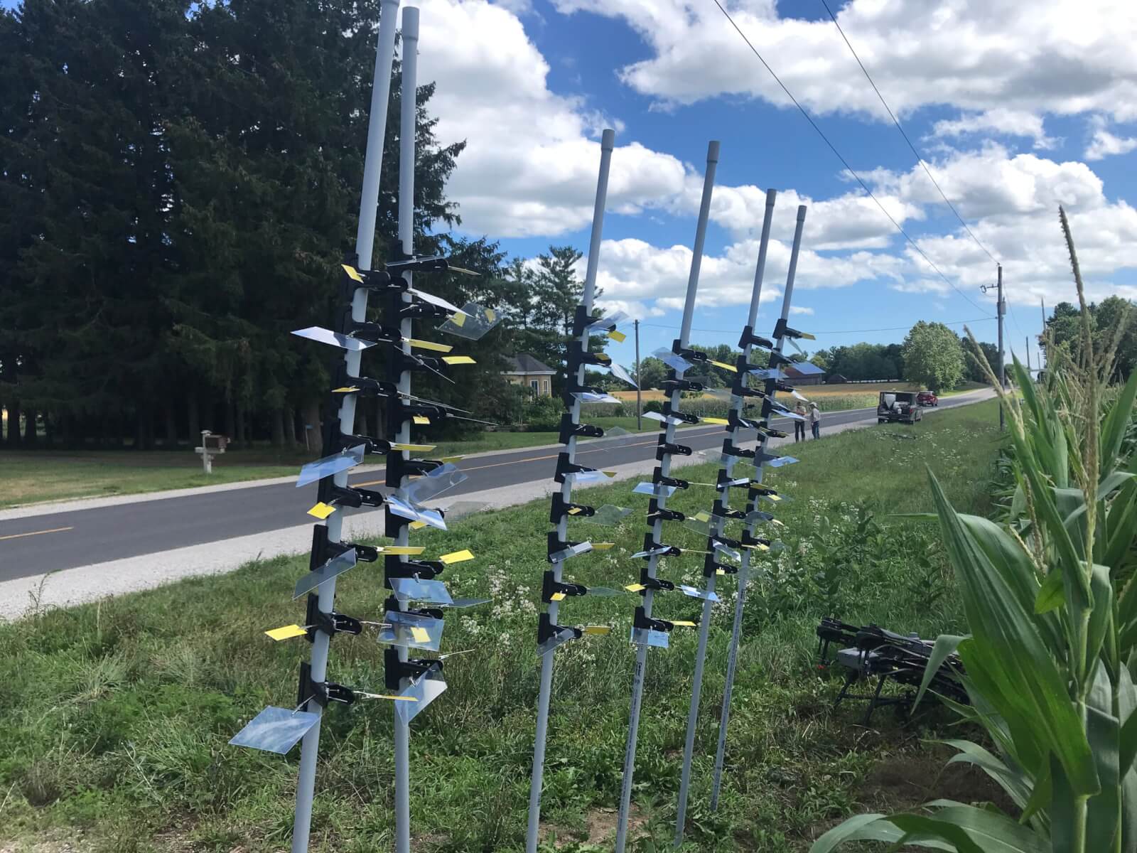
To account for variability, each treatment block was subdivided into two regions, each containing an array of nine spray collectors. Each spray collector (Figure 2) consisted of a vertical, 8’ pole in-row between corn plants. Samplers were attached at three depths to span the silking region: Top: 1.5’-2’ below the tassel. Bottom: 1.5’-2’ from the ground. Middle: halfway between them. Samplers were parallel with the ground to ensure the highest degree of spray interception. On one side, two 1”x3” water sensitive papers (WSP; Innoquest Inc.) were clipped back-to-back with a sensitive side positioned up (adaxial) and facing down (abaxial). The other clip held two 4” square sheets of Mylar in the same orientation. Sampler type was alternated vertically (e.g. Mylar – WSP – Mylar or WSP – Mylar – WSP).
Figure 2- Spray collectors temporarily loaded with WSP and Mylar samplers. These were held above the tassels as they were carried to the collection sites in each block. Three clips were positioned per pole, alternating Mylar and WSP samplers on each side, on two arrays of nine poles, as previously described.
This study used 864 WSP and 864 Mylar samplers for the RPAS treatments, and 162 WSP for the overhead broadcast and directed applications. Following the application, samplers were retrieved as soon as they were dry enough to handle (about 30 minutes) and individually placed into pre-labeled sealable plastic bags, each uniquely coded to the exact position and orientation of the collector.
Operational Use Cases
5 gpa: DJI Agras T10 was operated at 3.3 m/s, 2 m above tassels. TeeJet 11002 AIXR nozzles equipped with 50 mesh filters were operated at 70 psi.
2 gpa: DJI Agras T10 was operated at 7.0 m/s, 2 m above tassels. TeeJet 11002 AIXR nozzles equipped with 50 mesh filters were operated at 45 psi.
16.7 gpa: Overhead broadcast condition. Field 1 ran a John Deere 4038R operated at approx. 10 mph with TeeJet XR11006 nozzles on 20” spacing. Pulse width modulation (ExactApply) was engaged. Field 2 ran a New Holland 345 front-mounted boom sprayer with TeeJet XR11006 nozzles on 20” spacing.
20 gpa: Directed condition. John Deere R4038 operated at approx. 4.5 mph with Beluga drop hoses suspended on 30” centres to correspond with alley spacing. Two nozzle bodies were positioned 15″ apart equipped with Greenleaf Spray Max 110015 nozzles to span the silking area.
Drift Analysis
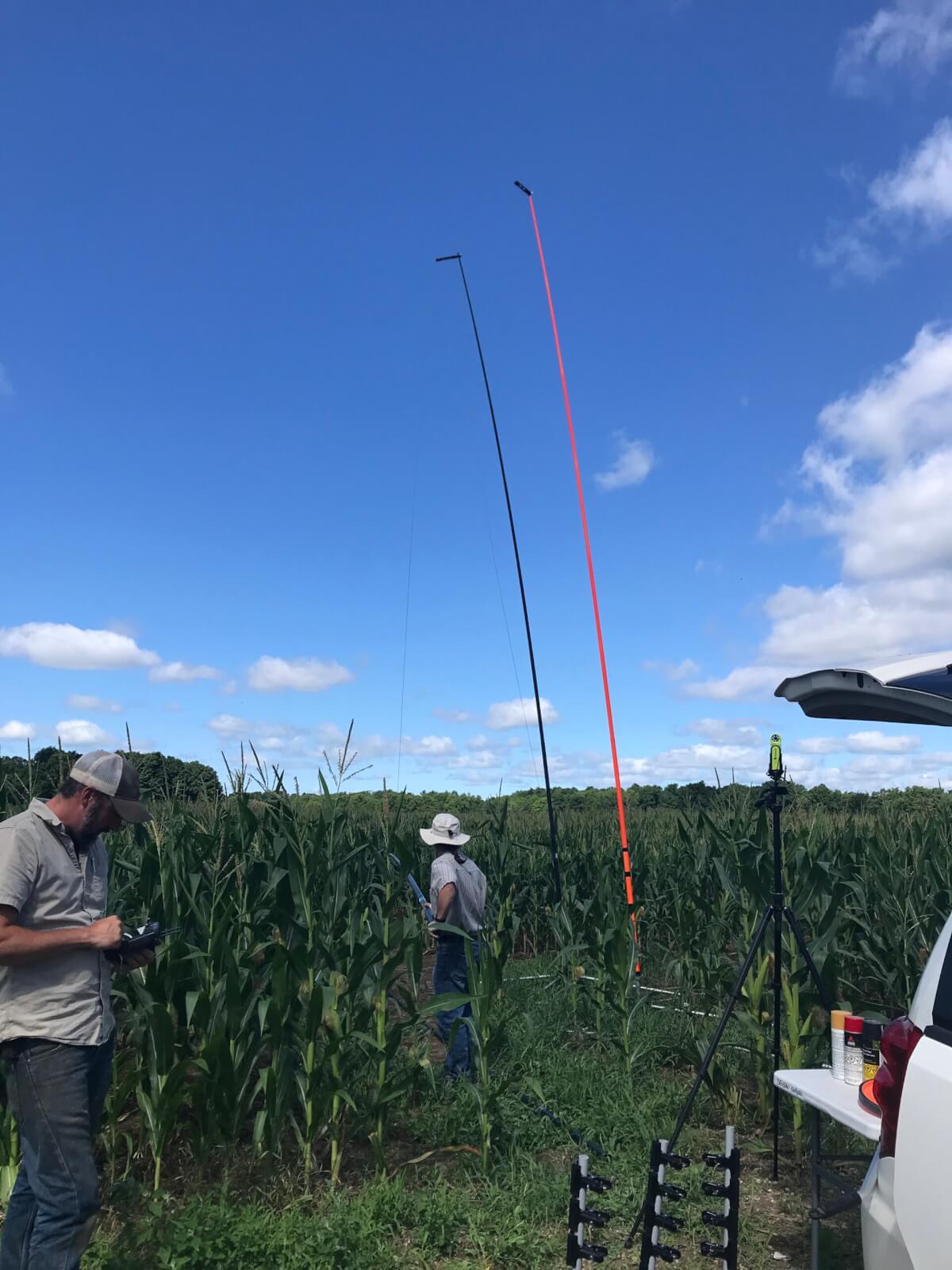
Three free-standing 26’ (8 m) horizontal flux collectors were positioned in the corn field approximately 3’, or 1.5 rows from the downwind edge of the spray plot downwind of the area treated by drone (Figure 3). The sampling poles were positioned about 30’ apart parallel to the treatment block. Sterilized, 1.8 mm braided polyethylene collector line was run up the poles on pulleys just prior to application. Following applications, the line was collected in 1 m lengths into sealed bags.
The assumption was that by placing the horizontal flux samplers as close to the “zero” downwind edge position as possible, nearly the entire off-swath movement of drift would be captured. A compromise of placing the samplers in the middle of the first row past the downwind swath edge was made due to the scale of the sample and the relative low swath precision of the drone. Placing the samplers closer to the zero downwind line was deemed to be too high a risk of inadvertently sampling in-swath.
Figure 3- Moving horizontal flux poles into the field prior to positioning them for trials. String collectors were run up the poles just before spray application and retrieved immediately afterwards.
Spray Solution (Formulated Product plus Tracer)
Fungicide was applied at field rates (8 oz/ac or 586 mL/ha). The field sprayer applied this at 16.7 gpa. The drone applied it at 2 or 5 gpa but also included tracer solution at 0.2% (20 ml/10L solution) vol./vol. of a 20% mass/mass solution of PTSA in dH2O. PTSA residue data assumes 100% recovery and 0% degradation of the tracer. Tests of PTSA with fungicide prior to the study showed no physical antagonism and >98% tracer recovery. Prior testing of PTSA showed an acceptable 1-2% solar degradation in the timeframe required to collect samplers. Tank samples were drawn from the drone at the beginning and end of each trial and used to confirm tank concentration and to establish fluorescence curves.
Weather Conditions
Weather data was collected using a Kestrel 3550AG weather meter (Kestrel Instruments) in a vane mount positioned 1 m above the tassel (approximately 1 m below drone altitude). Data was logged every 5 seconds. Issues with data loss required us to supplement local data with Field Level Weather Summary data (Table 2).
Date (2022)
Field
Vol. (gpa)
Avg. Temp. (°C)
Avg. Windspeed (km/h)
Start Time
Duration (min.)
Jul 25
1
5*
22.3
6.2
13:00
35
Jul 25
1
5
21.4
7.5
18:45
35
Jul 26
1
16.7
18.8
5.4
10:00
45
Jul 26
1
2
23.9
7.7
15:30
25
Jul 29
2
5**
n/a
16.4
11:00
35
Jul 29
2
2***
23.6
21.0
14:00
25
Aug 12
3
20****
25.4
6.3
13:30
15
Table 2- Date, location, and weather conditions for each treatment *Trial pass over spray collectors only – no horizontal flux collectors employed. **All bottom-level water sensitive paper samplers spoiled by high humidity. Wind changeable and horizontal flux poles moved 2x before application to orient downwind. ***Noted flocculation in tank samples likely from rainfastness adjuvant. Did not affect analysis. ****Coverage data from a single array of nine spray collectors with water sensitive paper samplers.
Results
Statistics
The % applied rate ac-1, % area covered, and deposits cm-2 were subjected to analysis of variance using SAS® OnDemand for Academics PROC GLM. When a significant treatment effect was found, means were compared using Tukey’s honest significant difference test (HSD) at p=0.05.
Data Collation
Each spray collector was a vertical structure that supported Mylar samplers at three depths. Each depth held two samplers oriented abaxially or adaxially, in parallel with the ground. When discussing the amount of PTSA recovered by sampler depth or by sampler orientation, the % applied rate ac-1 of each of the nine related samplers were averaged within each array (n=2 arrays per block times two replicates equal n=4 per treatment).
When considered from above, the six Mylar samplers are vertical cross-sections of the same area of ground. Therefore, the % applied rate ac-1from each sampler was added to represent the total mass of tracer intercepted per collector. When these nine sub-samples are averaged, we arrive at the average % applied rate ac-1 per array.
Similarly, the % applied rate ac-1 from each 1 m length of string on a horizontal flux collector could be averaged across collectors by relative position to explore drift by height (n=3 poles per block times two replicates equal n=6 per treatment). Alternately, the total PTSA recovered per pole could be calculated (n=3 poles per block times two replicates equal n=6 per treatment). This interpretation allowed us to perform a mass balance accounting of residue in-canopy and as drift compared to the known applied rate ac-1.
It was not possible to collate the data in this fashion for the WSP because it was not possible to index % area or deposits cm-2 on a 1”x3” area to a theoretical maximum. Therefore, we averaged the nine samplers within an array relative to their position and orientation (n=2 arrays per block times two replicates equal n=4 per treatment) or averaged the six samplers per collector prior to averaging all collectors in an array (n=2 arrays per block times two replicates equal n=4 per treatment).
RPAS Coverage – Mylar Samplers
There is a negative linear relationship (r2=0.997) between the depth of the sampler and the average % applied rate ac-1 (Table 3). The deeper the sampler, the less tracer recovered. The sum of the average % applied rate ac-1 at each depth was 17.7% of known rate applied rate ac-1.
Sampler Depth
Avg. % Applied Rate ac-1
Significance
Top
9.6
A
Middle
5.7
B
Bottom
2.4
C
Total:
17.7
–
Table 3- The depth of the sampler had a significant effect on the overall average amount of PTSA recovered.
The orientation of the sampler significantly affected the overall average amount of tracer recovered (Table 4). The abaxial surfaces intercepted an average 11.1 % applied rate ac-1 less (a 97% difference) than adaxial surfaces. Note: When Mylar was retrieved a few had physically shifted, potentially exposing the back side of abaxial collectors to primary deposition from above. Therefore, it is assumed that the actual deposit is lower than reported here.
Sampler Orientation
Avg. % Applied Rate ac-1
Significance
Adaxial
11.4
A
Abaxial
0.3
B
Table 4- The orientation of the sampler had a significant effect on the overall average amount of PTSA recovered.
When we separate the data to focus on the volume applied, we see volume had a significant impact on the amount of tracer recovered (Table 5). The average % applied rate ac-1 was 2.1% less (a 58% difference) in the 2 gpa condition compared to the 5 gpa condition.
Field
Avg. % Applied Rate ac-1
Significance
1
7.1
A
2
4.6
B
Table 5- The field location had a significant impact on the average amount of PTSA recovered.
When we isolate the volume applied by field, the 2 gpa treatment resulted in less coverage in field 2 (average 1.4 % applied rate ac-1 or 28% less) and significantly for the 5 gpa treatment (average 3.6 % applied rate ac-1 or 41% less: Table 6).
Date
Field
Volume (gpa)
Avg. % Applied Rate ac-1
Significance
Jul 25
1
5
9.2
A
Jul 26
1
2
5.0
B
Jul 29
2
5
5.6
C
Jul 29
2
2
3.6
B
Table 6- The average amount of PTSA recovered by date and location show lower overall recovery in Field 2.
When sampler depth is included in the field analysis (Table 7), we see similar deposition patterns; a negative linear relationship between coverage and canopy depth in all treatments save the 5 gpa treatment in field 2. Closer inspection confirms a reduction in coverage for the 2 gpa condition in field 2 versus field 1, and a significant reduction for the 5 gpa condition in field 2 versus field 1.
Table 7- The average residue recovered by date, location and sampler depth is significantly less in the 5 gpa condition in field 2 and does not distribute linearly by sampler depth.
RPAS Drift – Horizontal Flux
Overall, the volume applied had a significant impact on drift, where the 2 gpa treatment resulted in an average increase of 1.6 % applied rate ac-1 (44% difference: Table 8) versus the 5 gpa treatment.
Volume Applied (gpa)
Avg. % Applied Rate ac-1
Significance
2
3.6
A
5
2.0
B
Table 8- The volume applied had a significant impact on the amount of the PTSA recovered.
As with the Mylar samplers, there was a “field effect” where the field had a statistically significant impact on the amount of tracer recovered (Table 9). However, unlike the Mylar samplers in the crop, more tracer was recovered in field 2 (average increase of 3.2 applied rate ac-1 or a 67% difference) than in field 1.
Field
Avg. % Applied Rate ac-1
Significance
1
1.4
A
2
4.2
B
Table 9- The field location had a significant impact on the amount of PTSA recovered.
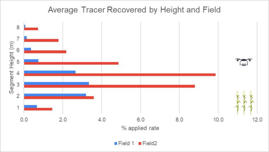
The pattern of deposition by height was similar across all treatments. For context, note that the first 2.5-3 m of string were within the corn canopy and drone altitude was approximately 5 m off the ground (2 m over the tassels) per Figure 4 and 5. The differences were only statistically significant in field 2 (Table 10) where an average 33% applied rate ac-1 was intercepted compared to 11% in field 1.
Figure 4- Average PTSA recovered (% applied rate ac-1) by height and field.Figure 5- Average PTSA recovered (% applied rate ac-1) by height and volume applied.
Height (1m segment in m from ground)
Field 1: Avg. % Applied Rate ac-1
Sig.
Field 2: Avg. % Applied Rate ac-1
Sig.
8
0.7
A
1.5
C
7
3.2
A
3.6
BC
6
3.3
A
8.8
A
5
2.7
A
9.9
A
4
0.7
A
4.9
AB
3
0.4
A
2.2
BC
2
0.1
A
1.8
C
1
0.1
A
0.7
C
Total:
11.2
–
33.3
–
Table 10- The average amount of PTSA recovered by height for field 1 and field 2.
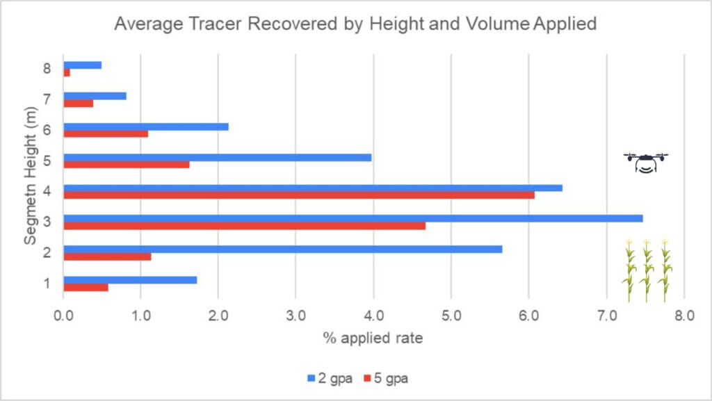
The volume applied had a significant effect on the total PTSA tracer detected in both fields, with an average 4.4% applied rate ac-1 more (a 59% difference) recovered in the 2 gpa treatment (Table 11 and Figure 5). Separated by fields, the 5 gpa treatment had an average 1.4% % applied rate ac-1 more (a 77% difference) in field 2 and the 2 gpa treatment had an average 2.8% % applied rate ac-1 more (a 76% difference) in field 2.
Volume Applied (gpa)
Field 1: Avg. % Applied Rate ac-1
Sig.
Field 2: Avg. % Applied Rate ac-1
Sig.
2
2.2
A
5.0
A
5
0.7
B
2.1
B
Table 11- The volume applied had a significant impact on the amount of PTSA recovered.
Mass Balance Accounting
It is never possible to entirely “close mass” in spray studies because there are other surfaces (e.g. leaves) within the vertical profile that intercept spray, as well as off-swath deposition and the ground itself (not measured in this study). Nevertheless, the exercise does allow us to estimate and compare how much spray was captured and how much remains unaccounted for (Table 12). We see that the 2 gpa treatment in field 1 had the highest unaccounted-for fraction, and on average we were able to account for an average 53% of the applied rate ac-1 in this study.
Field (Volume in gpa)
Coverage: Avg % Applied Rate ac-1 (A)
Drift: Avg % Applied Rate ac-1 (B)
Total % Detected (A+B)
Unaccounted Fraction [100-(A+B)]
1 (5)
51
5
56
44
1 (2)
26.5
17
43.5
56.5
2 (5)
30
24
54
46
2 (5)
19.5
40
59.5
40.5
Table 12- Closing mass using % PTSA detected on in-canopy samplers and on drift collectors.
RPAS and ground rig coverage – Water Sensitive Paper
The depth of the sampler had a significant effect on the overall average % area covered at all depths (Table 13). However, there was no significant difference at the two lower depths for deposit density (Table 14). In both cases, the negative linear relationship between coverage and sampler depth corresponds closely to the PTSA recovered on the Mylar samplers (see Table 3).
Sampler Depth
Avg. Coverage (% Area)
Significance
Top
2.80
A
Middle
1.28
B
Bottom
0.62
C
Table 13- Overall average % coverage by sampler depth.
Sampler Depth
Avg. Coverage (Deposits cm-2)
Significance
Top
44.5
A
Middle
17.9
B
Bottom
7.2
C
Table 14- Overall average deposit density by sampler depth.
The sampler orientation had a significant effect on both overall average % area covered (Table 15) and deposits cm‑2 (Table 16).
Sampler Orientation
Avg. Coverage (% Area)
Significance
Adaxial
3.03
A
Abaxial
0.12
B
Table 15- The orientation of the sampler had a significant effect on the average % area covered.
Sampler Orientation
Avg. Coverage (Deposits cm-2)
Significance
Adaxial
43.5
A
Abaxial
3.1
B
Table 16- The orientation of the sampler had a significant effect on the average deposit density.
The treatment had a significant effect on the overall % coverage (Table 17) with the overhead broadcast condition covering an average 3.31% more sampler surface (a 60% difference) compared to the next highest treatment value. The directed application delivered a significantly higher 67 deposits cm-2 (a 72% difference) compared to the next highest treatment value (Table 18).
Treatment (gpa)
Avg. Coverage (% Area)
Significance
Broadcast (16.7)
5.91
A
Directed (20)
2.32
B
Drone (5)
1.34
BC
Drone (2)
0.55
C
Table 17- Overall average % coverage by treatment.
Treatment (gpa)
Avg. Coverage (Deposits cm-2)
Significance
Broadcast (16.7)
92.6
A
Directed (20)
25.8
B
Drone (5)
22.9
B
Drone (2)
5.9
B
Table 18- Overall average deposit density by treatment.
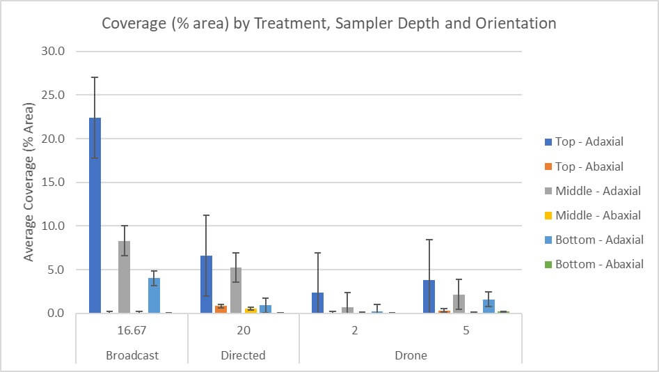
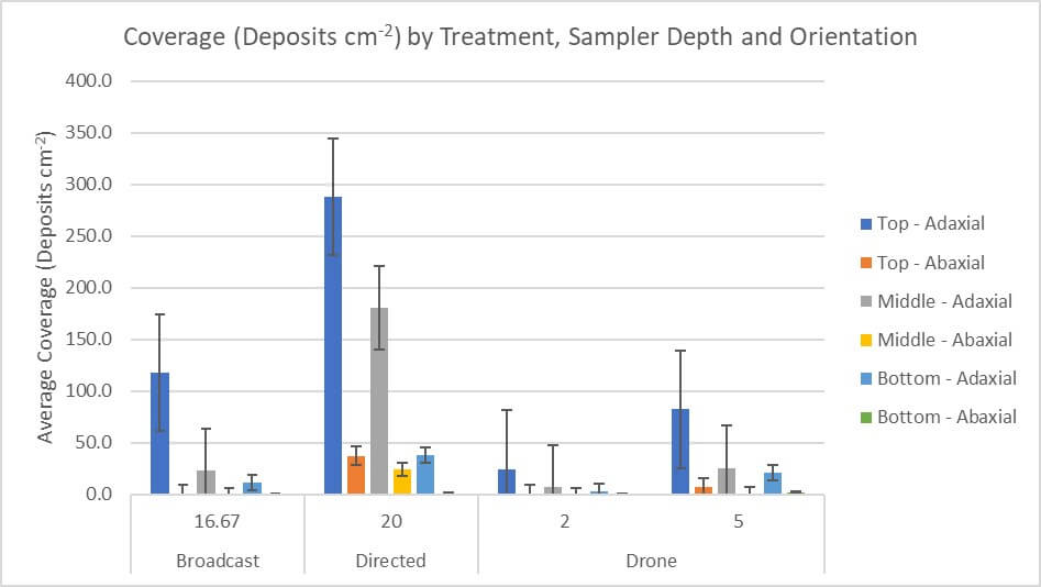
When we increase resolution to include sampler orientation, we see high standard errors typical of the variability inherent to spray coverage analysis (Figures 6 and 7). The broadcast treatment had the highest average adaxial % area coverage and the second highest average deposit density. The directed treatment had the second highest average adaxial % area coverage and the highest average deposit density but had the highest overall average coverage on the abaxial samplers. RPAS coverage on all samplers was lowest overall and was relative to the volumes applied.
Figure 6- Coverage (% area) by treatment, sampler depth and orientation.Figure 7- Coverage (Deposits cm-2) by treatment, sampler depth and orientation.
Focusing on RPAS treatments, the orientation of the sampler significantly affected coverage (Tables 19 and 20).
Sampler Orientation
Avg. Coverage (% Area)
Sig.
Avg. Coverage (Deposits cm-2)
Sig.
Adaxial
1.1
A
11.6
A
Abaxial
0.0
B
0.4
B
Table 19- RPAS (2 gpa) coverage by sampler orientation.
Sampler Orientation
Avg. Coverage (% Area)
Sig.
Avg. Coverage (Deposits cm-2)
Sig.
Adaxial
2.5
A
47.3
A
Abaxial
0.2
B
7.5
B
Table 20- RPAS (5 gpa) coverage by sampler orientation
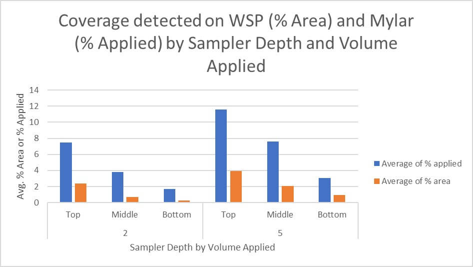
Continuing to focus on the RPAS treatments, the depth of the sampler had a significant effect on overall average coverage at both 2 gpa (Table 21) and 5 gpa (Table 22). Just as with the average % applied rate ac-1 (included here for comparison), the overall average coverage on the top adaxial sampler was significantly higher than the other two depths for % area covered and deposits cm-2.
Sampler Depth
Avg. Coverage (% Area)
Sig.
Avg. Coverage (Deposits cm-2)
Sig.
Avg. % Applied Rate ac-1
Sig.
Top
1.2
A
12.8
A
7.5
A
Middle
0.4
B
3.9
B
3.8
B
Bottom
0.1
B
1.3
B
1.7
B
Table 21- Coverage on the top sampler was significantly different than other depths at 2 gpa.
Sampler Depth
Avg. Coverage (% Area)
Sig.
Avg. Coverage (Deposits cm-2)
Sig.
Avg. % Applied Rate ac-1
Sig.
Top
2.1
A
48.3
A
9.2
A
Middle
1.1
B
17.6
B
5.8
B
Bottom
0.9
B
16.4
B
2.3
B
Table 22- Coverage on the top sampler was significantly different than other depths at 5 gpa.
Comparing data from WSP to Mylar Samplers
There was a correlation between the % area coverage detected using WSP and the tracer recovered from the Mylar samplers. Deposit density provides valuable information about the distribution of spray over the target surface but does not always correlate with % area covered, and it is therefore omitted from this comparison. When we plot the average % area covered from the adaxial WSP against the average % applied rate ac-1 from the Mylar samplers, we see the same near-linear pattern of decay with depth (Figure 8).
Figure 8- Average coverage from adaxial samplers plotted by depth and volume applied show similar coverage patterns.
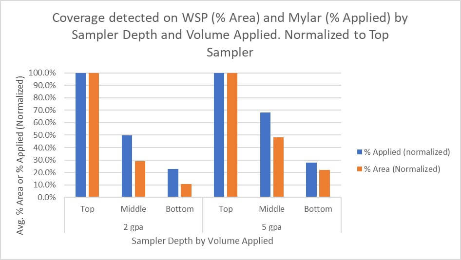
If we assume each top, adaxial sampler (irrespective of sampler material) represents the highest degree of coverage, we can assign it a value of 100% and index the data to this value. This allows us to visualize and compare the two sampler types directly (Figure 9) and illustrates similar relative coverage, but perhaps a greater rate of decay for the WSP.
Figure 9- Average coverage from adaxial samplers plotted by depth and volume applied show similar coverage patterns. Normalized to top sampler.
Net Revenue and Disease Pressure
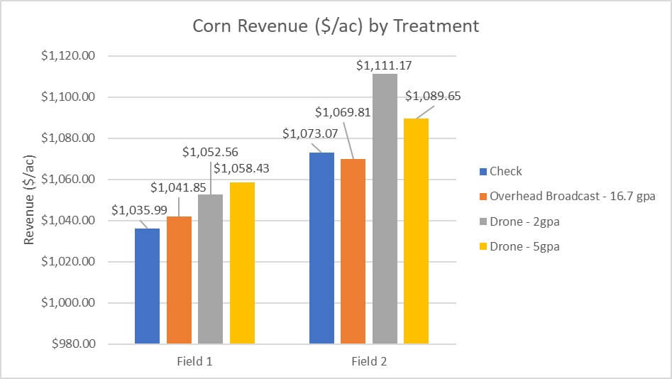
Crops were harvested at the R4 stage of development. There was no disease pressure detected in any field and no clear impact of application method on net revenue (Figure 10). Results based on the following formula: (CAD $/ac) = (Seed Yield × Corn Sale Price) – Drying Cost. No conclusions regarding efficacy can be drawn from this data.
Figure 10- Net Revenue (CAD $/ac) by field and treatment.
Key Observations
Water Sensitive Paper (WSP) measurements of percent area covered (% area) and deposit density (deposits cm-2), and Mylar samplers measuring mass deposit (% applied rate ac-1), revealed similar coverage patterns, making both samplers viable methods for RPAS coverage analysis. These are complimentary methods that reveal different aspects of coverage. When possible, they should be used simultaneously to produce a more complete analysis.
RPAS and conventional overhead broadcast applications produced similar deposition patterns in the corn canopy: A negative linear relationship between coverage and adaxial sampler depth was observed for most treatments (r2=0.997) and abaxial coverage was very low or more often, nonexistent. Further, overall coverage shared a direct relationship with volume for RPAS and conventional overhead broadcast applications.
Directed applications in this study employed a finer spray quality, released laterally from within the canopy. This produced a different coverage pattern than the RPAS and overhead broadcast applications. Per WSP, this treatment resulted in the highest overall deposit density and was the only treatment to produce significant deposition on abaxial surfaces.
For RPAS, spray coverage was significantly reduced by -58% (based on avg. applied rate ac-1), by -59% (based on avg. % covered) and by -74% (based on avg. deposits cm-2) and drift was significantly increased by +73% for the 2 gpa treatments versus the 5 gpa. We attribute this primarily to drone travel speed, which increased from 3.3 m/s at 5 gpa to 7 m/s at 2 gpa. For context, and with certain exceptions, travel speed shares a negative relationship with spray coverage and a direct relationship with drift in airblast and field sprayer applications.
There was a “field effect” where field 2 had lower overall RPAS coverage for both 2 and 5 gpa treatments. Compared to field 1, by -28% for the 2 gpa treatment, and by -41% for 5 gpa. Average drift increased by +76% for 2 gpa and by +77% for 5 gpa. We attribute this to the significantly higher wind conditions in field 2.
Given the lack of disease pressure in the two fields, and the lack of any significant difference in revenue by treatment within each field, efficacy is inconclusive. This study represented only two of eight fields in a larger RPAS efficacy trial where five locations had disease pressure high enough to rate. Preliminary results suggest that Tar Spot control from a 5 gpa drone application may be comparable to that of a 16.7 gpa overhead broadcast application from a field sprayer (data not shown).
Summary
Drone and conventional overhead broadcast treatments deposited spray in a similar pattern (a negative linear relationship with canopy depth and very low or no abaxial coverage), irrespective of the method used to analyze coverage. RPAS produced significantly lower coverage than the conventional overhead broadcast treatment, which is attributed primarily to the low volumes employed, per the direct relationship between volume applied and overall coverage (up to some point of diminishing return). High ambient windspeed significantly increased drift in both the 2 and 5 gpa conditions and reduced spray coverage. High travel speeds (required to apply 2 gpa) likely contributed to the significantly increased drift and reduced coverage in that treatment versus 5 gpa. For the use cases explored in this study, low volumes and high travel speeds are not advisable for RPAS, particularly in high wind conditions. Future work separating the travel speed and ambient wind speed variables would clarify their relative influence on RPAS drift and coverage.
This video presentation is covers the highlights of the study. And disregard the verbal slip-up: we didn’t travel 110 mph.
The decision on which application method is best for herbicides boils down to two main factors: (a) target type and (b) mode of action. In general, it’s easier for sprays to stick to broadleaf plants on account of their comparatively larger leaf size and better wettability compared to grassy plants. There are exceptions, of course – at the cotyledon stage, broadleaf plants can be very small and a finer spray with tighter droplet spacing may be needed. Water sensitive paper is a very useful tool to make that assessment. Imagine if a tiny cotyledon could fit between deposits – that could be a miss!
Some weeds are also more difficult to wet, and those may also need a finer spray or a better surfactant for proper leaf contact. An easy test is to apply plain water to the leaf with a spray bottle. If the water beads off or the droplets remain perched on top in discrete spheres, the surface is considered hard to wet. Most grassy weeds are hard to wet, while most broadleaf weeds are easy to wet.
Grassy weeds are an especially difficult target because they have smaller, more vertically oriented leaves, and almost without exception are more difficult to wet than broadleaf species. All these factors call for finer sprays for effective targeting and spray retention.
Broadleaf weeds usually have more horizontally oriented leaves which also happen to be larger. As a result, they can intercept larger droplets quite efficiently.
There are about thirty mode of action (MOA) groups among the herbicides with about ten accounting for the majority in Canadian prairie agriculture. It’s probably an over-simplification to categorize them into just two groups – systemic and contact. But that grouping goes a long way to making an application decision.
Contact products (MOA Group 5, 6, 10, 14, 22, 27) must form a deposit that provides good coverage. Good coverage is an ambiguous term that basically means that droplets need to be closely spaced and cover a significant proportion of the surface area because their physiological effects occur under the droplet, and don’t spread far from there. One way to generate more droplets is to reduce droplet diameter, another is to add more water. A reasonable combination of both is ideal because simply making droplets smaller creates issues with evaporation and drift.
Systemic products (MOA Group 1, 2, 4, 9) will translocate within the plant to their site of action after uptake. As a result, coverage is less important as long as sufficient dose is presented to the plant. In practice, this means coarser sprays and/or less water may be acceptable.
When two factors are combined, either in a tank mix or a weed spectrum, the more limiting factor rules. Application of a tank mix or product that is active on both broadleaf and grass plants will be governed by the limitation placed on grass targets. A tank mix comprised of both systemic and contact products is governed by the limitations placed on contact products.
A factor we should also consider is soil activity and the presence of residue. Studies have shown that soil-active products are relatively insensitive to droplet size. But if they have to travel through a layer of trash to get to the soil surface, more application volume is the best tool.
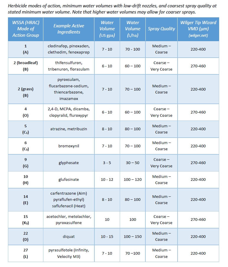
Below are some recommended spray qualities and water volumes for use in Canada. The spray qualities listed in the table can be matched to a specific nozzle by referring to nozzle manufacturer catalogues, websites, or apps. Note that Wilger also offers traditional VMD measurements on their site, allowing users to be a bit more specific if necessary.
One of the fastest moving new agricultural technologies is spray drones. Hardly a month goes by without some sort of new capability, some new features. It’s truly an exciting space to watch.
As with all things, there are good news and bad news to share. First the good news.
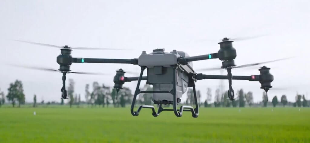
Drone capacity is on the rise. The early drones shipped with hoppers of 8 to 10 litres. Part of the reason was to keep weight below 25 kg. Below this weight, pilot licensing requirements and flight restrictions are easier. Anyone with a Basic RPAS license (RPAS is the official term for drones, Remotely Piloted Aircraft Systems) can operate drones up to 25 kg. Above this weight, one requires an Advanced license, which is much more difficult to obtain. Current drones like the DJI T40 have a hopper capacity of 40 L, allowing more area to be covered per flight.
The new DJI T40 holds 40 L of liquid and has a claimed swath width of 36 feet (Source: DJI)
Swath widths are increasing with drone size. The limiting factor for electric drones is still battery power. Flight times of 15 to 20 minutes are possible, depending on the ferrying distance. As a result, larger drones don’t necessarily fly longer, but they spray wider, up to a claimed 30 feet for the DJI T30, and 36 feet for the T40.
Atomizers are improving. The trusty flat fan nozzle certainly works on a drone, but its proper operation depends on spray pressure. And spray pressure is not currently reported by drones. Instead, their application software relies on flow rate, and pressure is adjusted in the background in response to changes in travel speed, swath width, or nozzle size. Although drone flow meters are remarkably accurate, the operator could inadvertently operate the drone at a pressure that produces the wrong spray quality for the conditions.
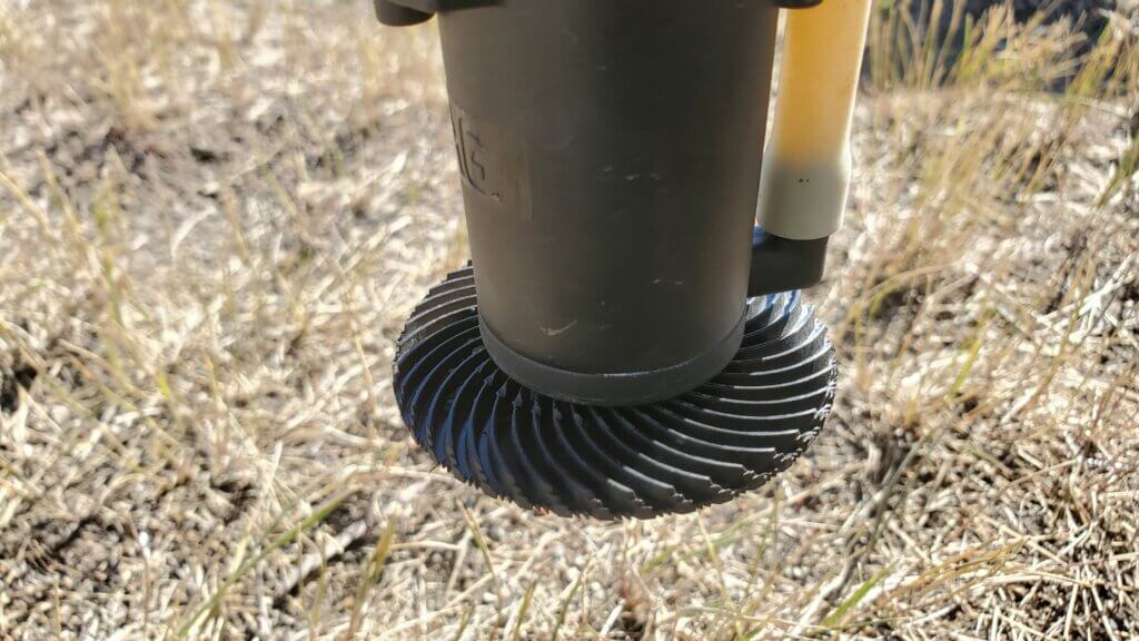
Enter the rotary atomizer. Long a darling of the thinking applicator, these atomizers use centrifugal energy to create a spray with a tighter span, meaning fewer fine and fewer large droplets. Spray quality still depends on pressure-generated flow rate, but droplet size can additionally be altered with rotation speed. This means that if a faster travel speed increases the spray pressure, the effect on spray quality can be counteracted with a changed rotational speed to keep everything more uniform.
Rotary atomizers, like this one from XAG generate more uniform droplet sizes and can alter droplet size without changing spray pressure.
Hybrid systems are entering the market. Rotary wings allow for precise positioning of aircraft and they provide downwash that helps spread the spray pattern out. Downwash also improves canopy penetration and could reduce drift, like air-assist, if used properly. But rotary wings use a lot of energy, limiting battery life. When flown at the wrong height or speed, deposit patterns, drift, and swath width will change. That has to be managed and requires experience.
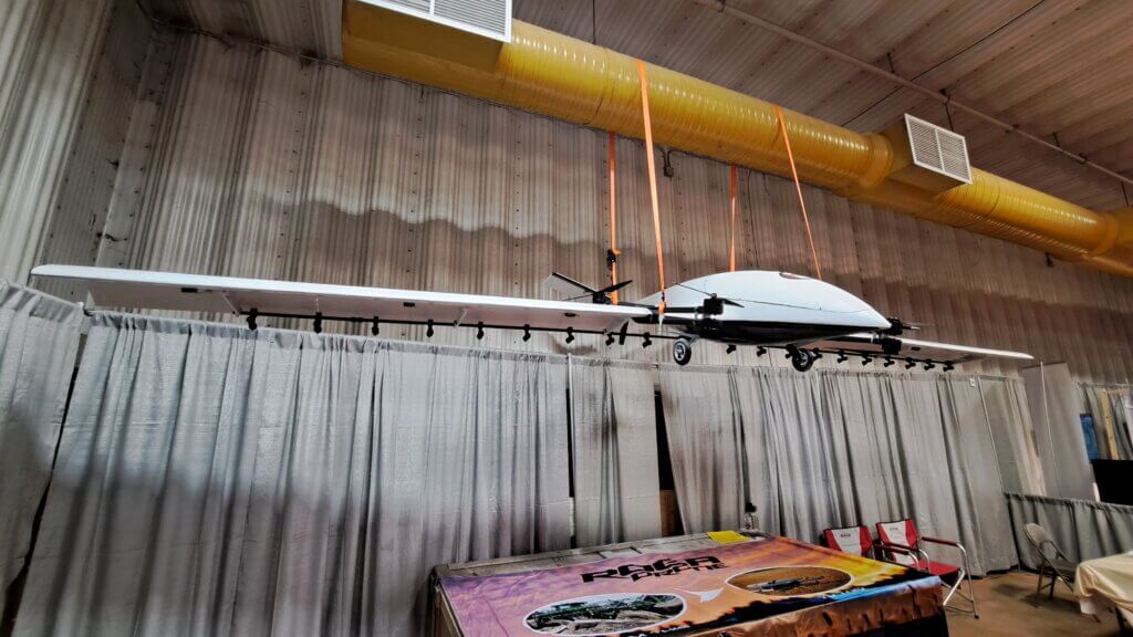
In comparison, hybrid drones have fixed wings for flight and rotary wings for take-off and landing. The rotors just rotate into the position needed at the time. Fixed wing drones will fly faster, possibly improving capacity and also reducing the effect of the downwash. These systems are new, and much needs to be learned before we understand their various characteristics. But they offer a nice avenue into more productivity.
Hybrid drones like this one from Advanced Robotics can cover more ground with less turbulence than a rotary wing drone.
Drones are multi-purpose. Virtually all drones have interchangeable wet and dry hoppers so they can be used to apply dry nutrients or seed as needed. That makes them quite versatile. But the newest spray drones have scouting-quality cameras on board and can be asked to take high resolution images while they’re spraying. At the end of the mission, a very detailed picture of the crop emerges, with much higher resolution than the higher-elevation scouts produce. Other sensors on the drones can be used for variable rate application of nutrients, or even for spot spraying weed patches.
Scouting camera takes pictures while conducting a spray mission (Source: DJI)
Now for the bad news. It’s still not legal to apply mainstream pesticides using drones in Canada, and it may stay that way for a while yet.
Pesticide application by drones remains illegal in Canada. The main reason is that the Pest Management Regulatory Agency (PMRA) has declared drones to be unique application method, separate from ground sprays and aerial sprays from piloted aircraft. This has triggered the need for risk assessment data for spray drift, efficacy, bystander exposure, crop residue. It’s a fair decision – drones produce finer sprays than any other existing system, they potentially use lower water volumes by necessity, and they create a less predictable deposit due to rotor downwash. The majority of current pesticide formulations are designed for 5 to 10 gpa, this creates a certain concentration of surfactants and products that interact with plant surfaces or that change the potency of drift. Altering this by a factor of 5 can have undesirable outcomes. Yes, aircraft also use lower volumes, but more in the area of 2 to 5 gpa. Drones could cut that in half again, and that warrants study.
Registrants haven’t rushed to study drones. Most major manufacturers of pesticides have a small drone program to get their feet wet, and most have applied for Research Authorization (RA) from the PMRA to study them. But the decision to register a drone use for a pesticide has much to consider. Is it worth it to generate the required dataset for the regulators? Will drones amount to a lucrative new market for product? Do we have the resources and expertise to service this new market? The answers to such questions are clearly complex and much remains unknown. The registrants’ caution is understandable.
There may be a small portfolio of available products. Anyone thinking that a fleet of inexpensive, nimble drones will replace their ground sprayer is banking on the registration of the products they need in their operatioin by the registrants. The most likely products to be registered are fungicides, for which drones would offer several advantages in canopy penetration and spraying in tight time windows due to, say, wet weather.
Another obvious use is in industrial vegetation management where rough terrain or remote locations make it difficult to use wheeled sprayers. Or vector control with larvicides, which, incidentally, comprise the first pesticide registrations for drones in Canada (two microbial mosquito larvicides were approved for drone use in October 2022).
But it seems unlikely in the short term that a producer would have their pick of products to apply by drone anytime soon. And this means that a drone would remain a supplemental tool on the farm, not the main workhorse.
Regulatory hurdles are substantial. Not only is a pilot required to be licensed to use drones, a pesticide application also requires a Specialized Flight Operations Certificate (SFOC). In general, SFOCs are required if:
you are a foreign operator (i.e., not a Canadian citizen or permanent resident);
you want to fly at a special aviation event or an advertised event;
you want to fly your drone carrying dangerous or hazardous payloads (e.g. chemicals);
you want to fly more than five drones at the same time.
SFOC applications are fairly easy to fill out. Aside from identifying the drone and the pilot, the application needs the purpose of the mission, the location of the mission, and the time period of the mission. The problem is that it may take up to 30 days to hear back for simple missions, 60 days for complex mission. And if the SFOC is not granted, you can’t fly. You can’t decide to spray a field at the last minute.
The news is clearly a mixed bag. We have it all – exciting technology, obvious niche in the marketplace, significant regulations, slow process. In the meantime, spray drones are legal to purchase and relatively inexpensive. And we know they are being purchased. Canada doesn’t have a strong compliance system within the PMRA, so it’s hard to know how much pesticide spraying is being done illegally, or how perpetrators will be treated by the law.
The reputation of the industry once again rests with hope that good decisions are being made by conscientious individuals.