Introduction
Spray coverage describes the degree of contact between spray droplets and the target surface area. This metric can be used to predict the success of an application. One of the easiest methods for visualizing coverage is to use water sensitive paper (WSP), which is a passive, artificial collector that turns from yellow to blue when contacted by water.
WSP is often used to evaluate iterative changes to a spray program. Placed strategically throughout a target canopy, or directly on the ground, achieving uniform, threshold coverage translates into improved efficacy, reduced waste, reduced off-target contamination and reduced risk of pesticide resistance development. WSP were also used to develop a system that measures the area covered by the effective radial distance in an attempt to relate the area covered by a stain to a larger area where sufficient pesticide activity is taking place.
WSP tends to underestimate the spreading effect that can occur on plant surfaces (especially when surfactants are used), but they are effective as a relative index.
A brief history of WSP
In 1970, a journal article described a new method for sampling and assessing spray droplets. Photographic paper treated with bromoethyl blue created a yellow surface that changed colour when it encountered moisture. The pH-based reaction was fast and irreversible, leaving a distinct blue stain to mark the deposition.
Ciba-Geigy Ltd. made water sensitive paper commercially available in 1985 (later as Novartis in 1996 and as Syngenta since 2000). It is produced in several formats, but aluminum foil packages of 50, 76 x 22 mm (1 x 3 in.) papers are the most popular. Odds are if you’ve ever used water sensitive paper, it originated from Syngenta in Switzerland. In 2023 I noticed that the papers now say “made in Germany.”

In recent years, two new options have been made commercially available: Innoquest’s SpotOn Paper (United States) and WSPaper (Brazil). At the time of writing, there has been no impartial comparative evaluation of these three products.
Once dry, the blue stains on WSP are irreversible and papers can be stored for long periods of time. However unstained portions will continue to react to moisture from humidity, dew, or fingerprints, so care must be taken in their handling and storage.
Comparing WSP brands
The three commercially-available brands of WSP were subjected to a series of comparisons. The intention was not to rank these products, but to determine if they performed in a similar fashion and to alert users to any significant differences.
Packaging and Appearance
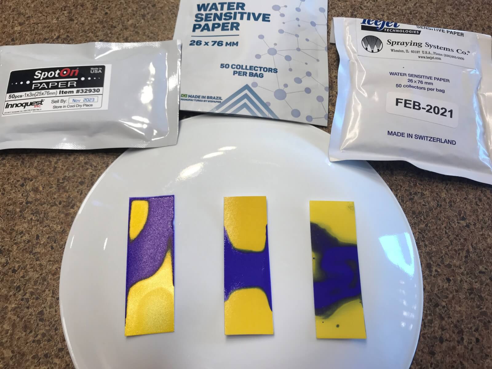
Each package was donated for the study. The SpotOn (SO) papers had a “sell-by” date of November 2023, the Syngenta (SY) papers (provided via Spraying Systems Co.) were dated February 2021 and the WSPaper (WS) was their newest formulation (white package, not silver), received June 2021. The comparison was performed on July 5, 2021.
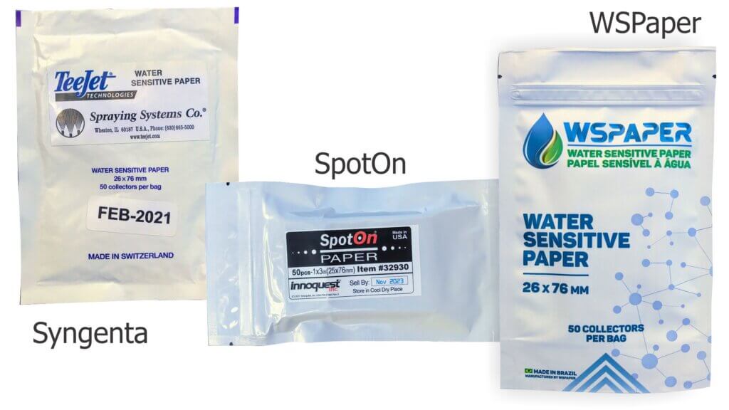
Each product was a foil or plasticized bag of 50, 26 x 76 mm papers. SO and WS had a re-sealing feature similar to that of a sandwich bag. SO also included a package of silica gel desiccant to capture moisture and a pair of plastic forceps to facilitate handling.
Users are encouraged to label papers to ensure they know their relative position and sprayer pass for later analysis. It was possible to write in ink on the faces of the SY and SO papers, but not WS. It was possible to write on the back of all brands.
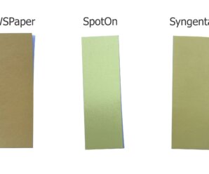
The three papers were different shades of yellow. Further, in the author’s experience, the colour can be visibly different between batches of the same brand. In the case of larger experiments where more than 50 papers are required, it would be prudent to ensure papers are not only from the same manufacturer, but the same production batch. This would not be an issue when subjectively comparing papers, but when using software that employs colour thresholding to identify deposits, it could create artifacts. Presently, only Syngenta has a batch number (found on a sticker on the back of the bag).
Bleed-through
WSP is often placed in foliar canopies which are subject to dew and transpiration that can cause the papers to react prematurely. This can be particularly limiting when moisture soaks through the backs of papers. Each brand of paper was placed face-up on a drop of water to see if the water would bleed through.
WS quickly curled as the water wicked in from the edges. Within five minutes the water soaked through from the back as well. Within five minutes SY also curled, but the colour reaction was entirely due to water soaking through and not wicking along the edges of the paper. SO did not curl and there was no colour reaction save a minor wicking reaction at one edge. It did however produce a dark yellow patch. In order to see if a colour reaction was still possible, a single drop of water was placed on the face and the colour reaction was distinct and instantaneous.
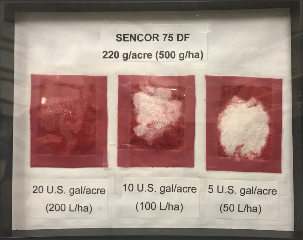
Note: Others have since replicated this experiment and reported that the response depends on the amount of water used and how long you leave it. We repeated our experiment with higher volumes and longer wait times (see image below). Ultimately, no brand of WSP is water proof from the back. Nevertheless, with small volumes of water (such as from dew) the original assessment of each brand is still valid.
Deformation and drying time
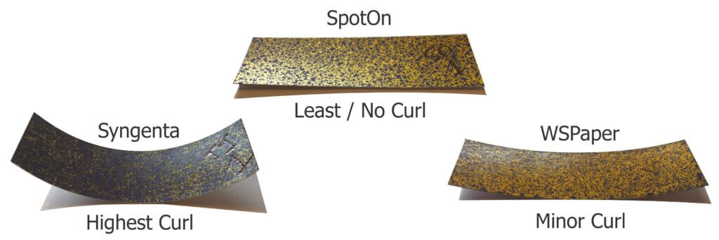
Users of water sensitive paper may be familiar with its occasional tendency to curl when one side is sprayed. In extreme cases, this movement could create smears if the paper contacted other wetted surfaces in dense foliage. The degree of curling was significantly different by brand, with SY becoming convex when wet and then flexing back into a concave form once dry. WS deformed as well, but only to a minor degree. SO did not appear to deform at all. Syngenta has noted that the degree to which their papers curl depends on the batch. Their manufacturing process has changed over the years in response to regulatory requirements and minor adjustments are still occasionally made.
There was no appreciable difference in the time it took for any brand to dry. This is based on attempts to smear papers every 30 seconds. All were dry in under five minutes.
Experimental design
While there is considerable variability inherent to spraying, every effort was made to maintain consistent conditions. Papers were sprayed in a closed room with no appreciable air currents (21.5 °C and 64% RH). Papers were paired randomly, side-by-side on a plastic sled. The sled was pulled at 2.5 kmh (~1.5 mph) through the centre of a spray swath produced by a TeeJet XR80015 positioned 50 cm (20 in.) above the targets. The nozzle operated at 2.75 bar (40 psi) to produce ~270 L/ha (~29 gpa) with Fine spray quality. Six passes were made, producing four sprayed papers for each brand.
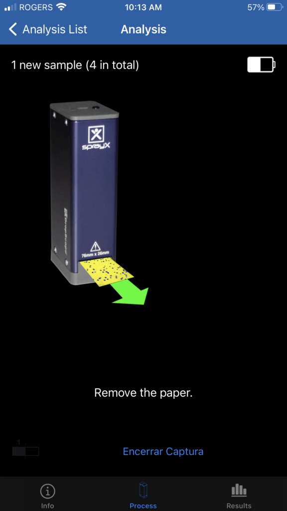
All papers were dry to the touch after two minutes. They were removed to a cooler, low humidity space and were digitized and analyzed using the SprayX DropScope (v.2.3.0) within an hour of spraying. We noted that while WS and SO fit easily into the DropScope port, the SY papers were sometimes slightly wider and had to be forced. Learn more about how to digitize and analyze WSP in this series of articles.
The “ground” option was selected, and each brand of paper was processed using its specific spread factor. DropScope has a detection threshold of 35 µm. This is appropriate as the smallest droplet diameter that can be resolved by any brand of WSP is ~30 µm (Syngenta, Innoquest, SprayX – Personal Communication).
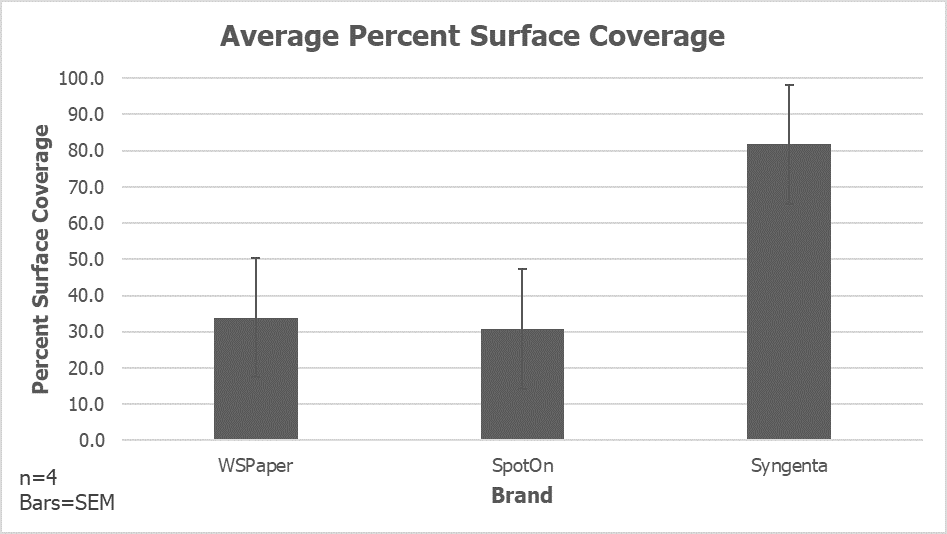
Percent surface covered
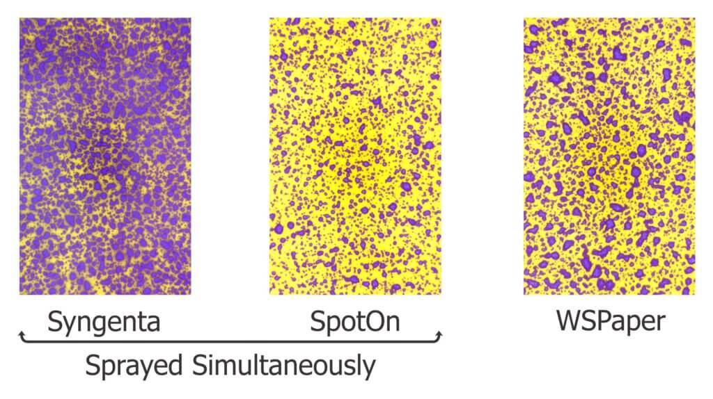
The average percent surface covered was calculated with standard error of the mean for each paper. WS and SO produced similar values between 30 and 35%. While all three brands exhibited similar variability, SY approached saturation at approximately 80% coverage. Therefore, WSPaper exhibited a slightly higher degree of spread than SpotOn, while the Syngenta paper exhibited a significantly higher degree of spread.
For reference, it can be difficult to determine if a stain represents a single deposit or is the result of multiple overlapping deposits. This becomes a problem when the surface of the WSP exceeds 20% total coverage. Further, it becomes increasingly difficult to distinguish a stain from the background, unstained surface when papers exceed 50% total coverage.
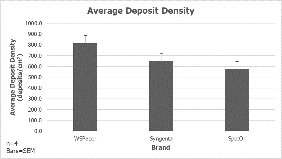
Deposit density
The average deposit density is a count of discrete objects (i.e. stains) per cm2. WS appeared to resolve the highest count, followed by SY and then SO. The process for determining what is a discrete object, and not the result of anomalies such as overlapping deposits, elliptical deposits or imperfections in the paper itself is complicated and computationally heavy. The algorithms employed by DropScope treated each paper consistently. So, while some differences are attributed to variations in spraying, they also reflect the paper’s innate ability to resolve individual deposits.
Droplet diameter
It is not the intent of this article to determine if WSP should be used to extrapolate the original droplet size. The many assumptions and inconsistencies inherent to this process are well known. Nevertheless, some researchers do use WSP in this manner, so a comparison was warranted.
DropScope bins deposit diameters by size to produce histograms of deposit size by count. These stain diameters are used to extrapolate DV0.1, DV0.5 (VMD), DV0.9 and NMD, which describe the population of droplets that produced the stains. DV0.5 is the Volume Median Diameter, or the droplet diameter where half the volume is composed of finer droplets and the other half by coarser droplets. Number Median Diameter (NMD) is the droplet diameter where half the total droplets are finer, and half the total droplets are coarser.
Each brand of WSP will permit a certain degree of spread when a droplet of water contacts the surface. This spread factor is specific to the brand of paper. Further, the spread factor is not constant for all droplet sizes; Finer droplets will spread less than coarser droplets.
When processing data using DropScope, selecting the appropriate spread factor makes a significant difference to the output. For example, here are the same four SY papers processed using the Syngenta-specific spread factor as well as the spread factors intended for SpotOn and WSPaper.
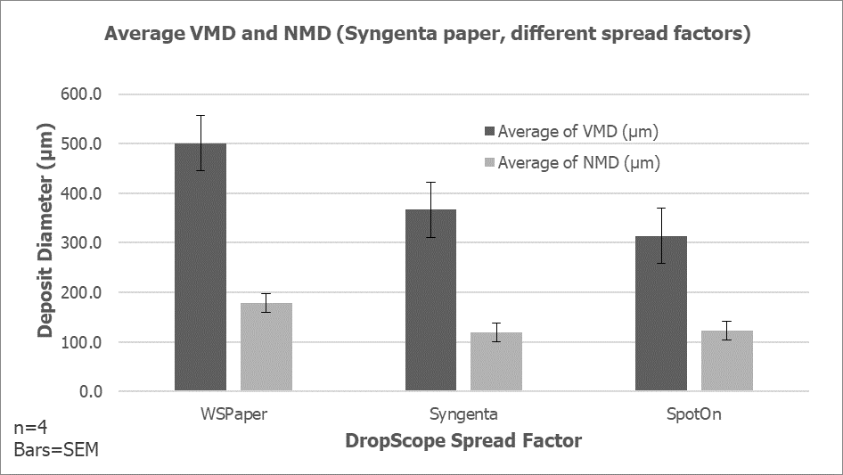
Therefore, each brand of water sensitive paper was analyzed using its brand-specific spread factor (according to DropScope), to produce the following graph.
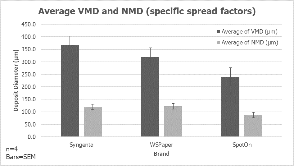
SY produced a VMD higher than that of WS, and both were higher than SO. There was less variability in the NMD, but this was expected given the high droplet count on the finer side of a hydraulic nozzle’s droplet size spectrum.
Conclusion
Water sensitive paper has immeasurable value in agricultural spraying. It is far more important to encourage its use than to quibble over brands. However, when these tools are used for more rigorous evaluations of spray coverage, brand-specific variability must be addressed.
The differences in how each brand responds to moisture (i.e. discolouration and deformation) may factor into which brand is most appropriate for a given situation. Further, there appear to be significant differences in how each brand resolves coverage. Once again, this may be irrelevant for those spray operators who occasionally use WSP to inform their spraying practices, but for consultants and researchers it is suggested that they use a single brand for an experiment, with papers produced in the same batch run.
Syngenta, Spraying Systems Co., SprayX, WSPaper and Innoquest are gratefully acknowledged for their contribution of materials and time informing this article.
2026 Update
If there’s one thing that stays the same, it’s that nothing stays the same. Formulations and manufacturing processes change. According to SprayX, manufacturers of the DropScope, all three of the papers described in this article (written in 2021) have changed in recent years. Some have improved and others can create potential errors in digitizing coverage. The following points may require a deeper understanding of how WSP is digitized and analyzed. Refer to this series of three articles.
Be aware of the following best practices when using WSP:
- Be aware of package expiration dates. Expired paper will work differently from new paper, creating an artifact in analysis.
- Papers with bright, reflective surfaces can cause an underestimation of deposit counts (specifically the smallest deposits).
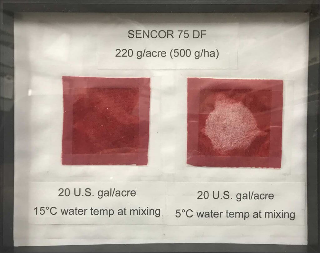
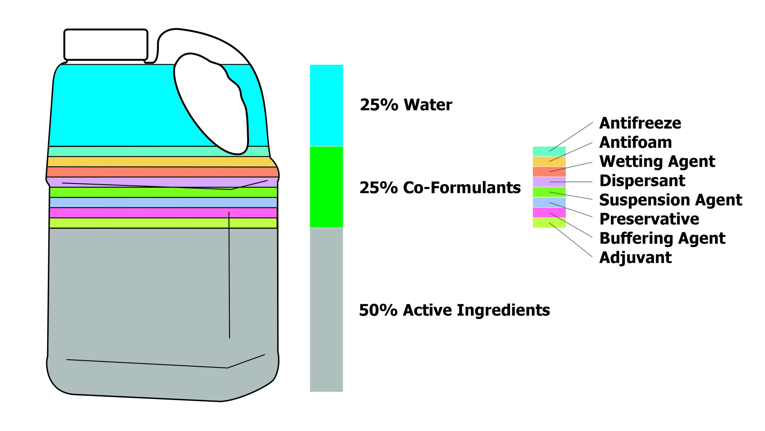
- Best results are obtained when using water for testing. Adjuvants and pesticide co-formulants have minor impacts on spread, but can also change the how the paper changes colour, making thresholding difficult.
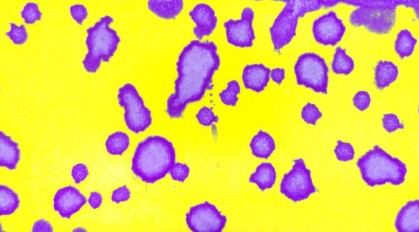
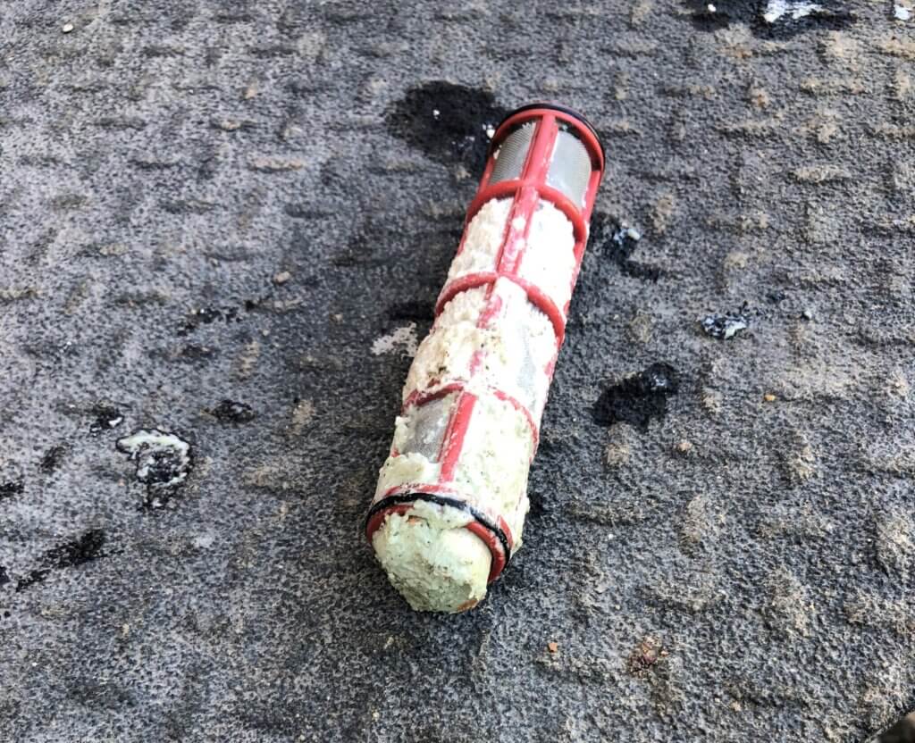
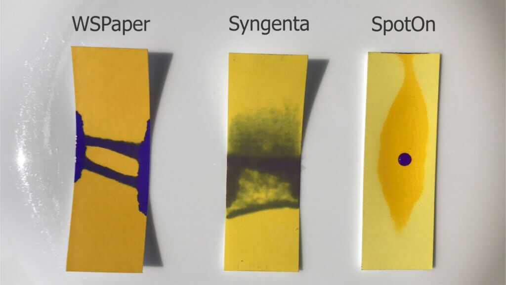
- Beware papers that create stains with bright borders and faint (hollow) centres (see image below). This can lead to an underestimation of volume median diameter. If your camera or scanner permits, examine the coverage in binary (e.g. black and white) for more accurate results.
- Do not sample the edge of the WSP (leave at least a mm) to avoid edge effects such as wicking and partial impacts. Some scanners have a setting, or you can select the area manually.
- Note the physical shape of the paper itself. Inconsistencies in the length and width (cutting errors) can make papers difficult to use in certain scanners, and curled papers cause changes in perspective and focal distance that can lead to errors.
- When not using a sealed camera or scanner (e.g. DropScope or flatbed), changes in the camera angle, shadows, lighting conditions, and make/model of cellphone camera will affect the results. Be consistent.