We’ve been here before, haven’t we? I could rehash the explanation of why wheat head coverage is important, and define the variables involved, but perhaps you’re already in-the-know. Instead, new readers (and those requiring a refresh) can go give this article and this article a quick read and then come back. I’ll wait.
Why perform another wheat head nozzle assessment? Primarily we do it so you don’t have to, but in this case there’s a specific problem we’re trying to solve and a “new” nozzle to explore.
The problem (and some history)
Let’s digress a little and use the historical experience shared by Clean Field Services (CFS) in Drayton, Ontario (cooperators in this study), to explain the problem and our objective.
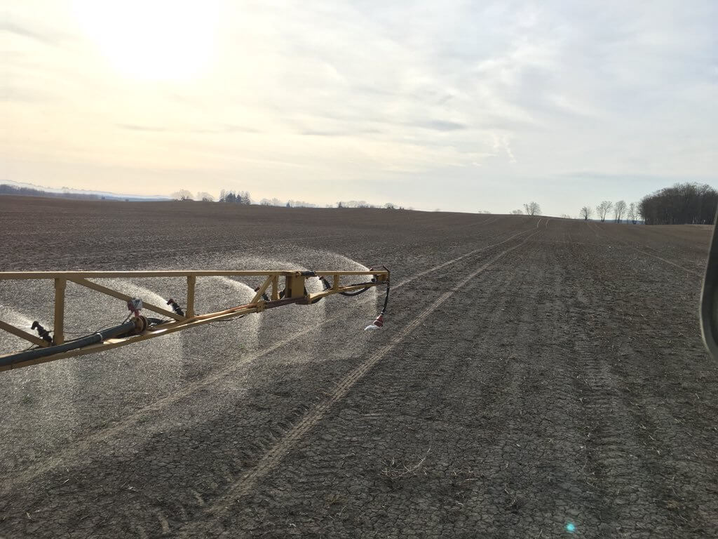
As broadacre sprayers evolve, nozzle technology has been lagging. Consider a basic field sprayer equipped with a centrifugal pump. Its performance curve exhibits a direct relationship between flow rate and pressure. In this case, the operator relies on a rate controller to bypass flow to maintain a target application rate across a range of travel speeds.
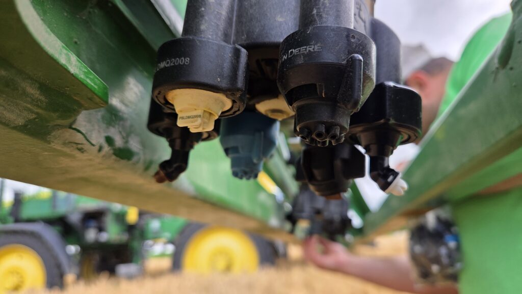
However, bypassing changes system pressure, which inadvertently changes the average droplet size. Basically, increasing travel speed reduces droplet size and vice versa. This was the manner of sprayer used in Ontario more than 20 years ago when researchers demonstrated that TeeJet Turbo FloodJets, alternated front-to-back, provided excellent coverage of wheat heads at the T3 timing. This is what Clean Field Services used.
However, some booms have obstructions that interfere with the aggressive spray angles produced by wide-pattern nozzles such as the Turbo FloodJet. CFS experienced this when they got a RoGator in 2012 and later an R-series Deere in 2017. At one point they tried using extensions to clear the obstruction, but this proved to be a nuisance and interfered with folding. They settled on GreenLeaf Technologies’ TurboDrop Asymmetric DualFan (TADF), which worked great, until the sprayer changed again.
Pulse Width Modulation
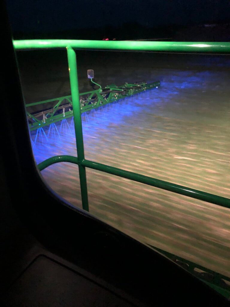
Sprayer plumbing and control systems have evolved. The introduction of pulse width modulation (PWM) technology changed the way rate control is achieved. Rather than regulating flow by altering pressure, PWM intermittently interrupts flow at the nozzle. This decouples flow rate from pressure, preserving droplet size across a range of travel speeds. Most air induction (AI) nozzles, such as the TADF are not approved for use with PWM systems.
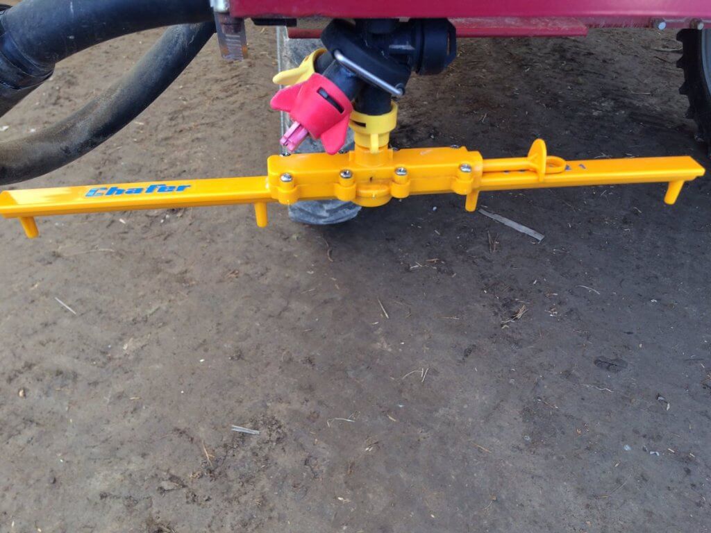
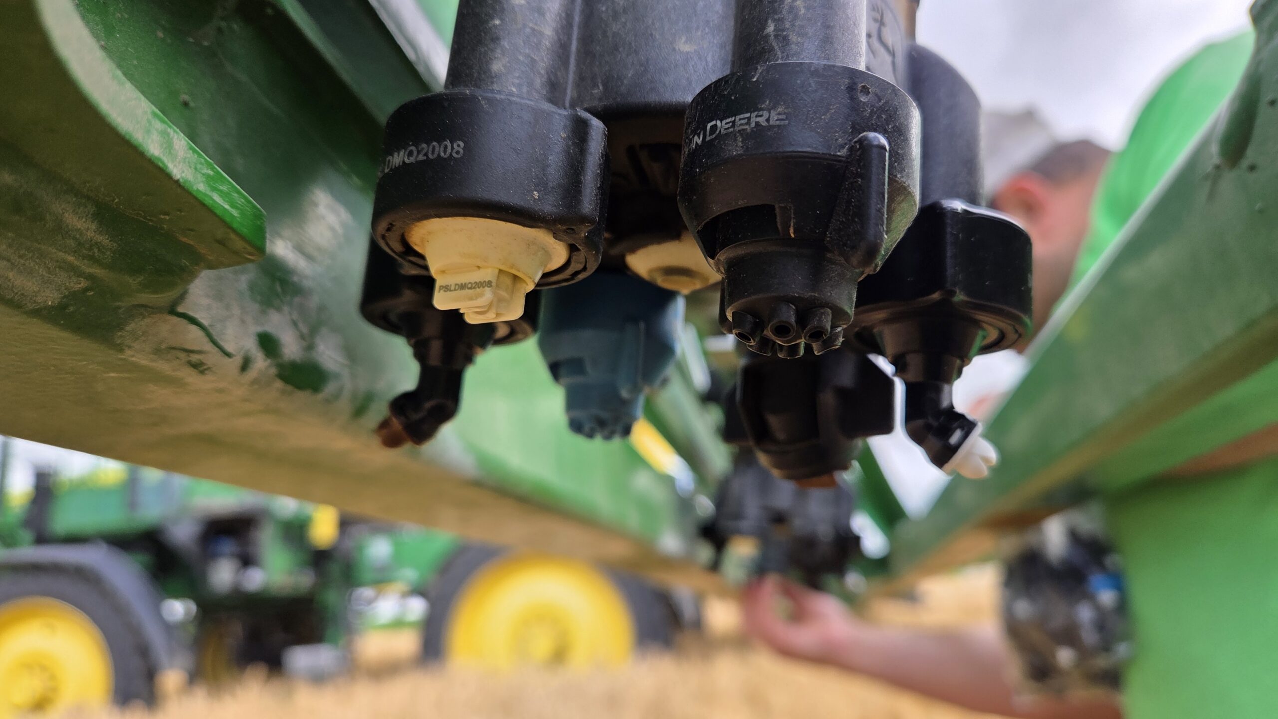
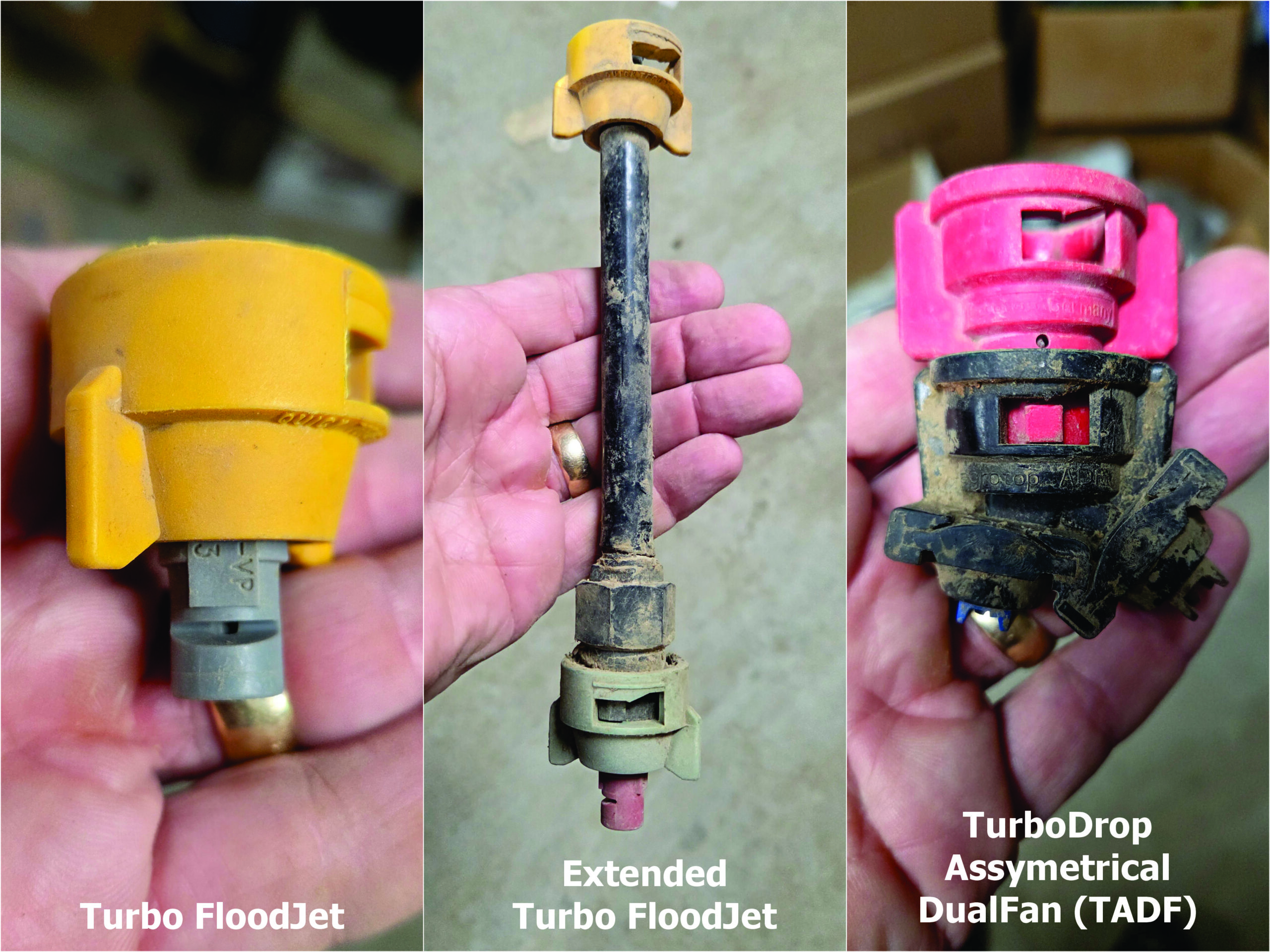
John Deere’s ExactApply PWM system became available in 2017, and CFS got one in 2018. Operators could mount two nozzles in each position, creating opportunities for interesting new configurations. One of the recommended nozzles was the Defy 3D, which features a 38° angle and was developed by Hypro in collaboration with Syngenta to help control blackgrass in the UK. It performed well in drift-reduction studies relative to conventional flat-fan nozzles.
Welcome to Canada
CFS mounted a single Defy 3D ’08 in each nozzle body, and had problems. Canadian sprayer operators, on average, drive faster than their UK cousins. Even with PWM, the largest Defy 3D tip (the ’08) required a flow rate that increased system pressure, which in turn led to a drifty experience. Bad in itself, but also not ideal for angled applications, because finer spray deposits with the wind rather than ballistically.
They tried throttling back, slowing down and/or adjusting water volumes, but felt they never really dialed it in. They settled on a Defy 3D ’08 in the B (rear) position, and an ’05 in the A (front) position at 21 km/h (13 mph) to apply 156 L/ha (16.67 gpa).
Exploring a solution
Wouldn’t it be nice to have your cake and eat it too? Drive faster, apply higher volumes and still mitigate drift? Enter the 3D Ninety, with claims of good fungicide utility while producing a significantly coarser droplet than the Defy. They came out in 2021, and yet they are still difficult to find in North America. This study establishes baseline panoramic coverage from the Defy 3D, then benchmarks it against the 3D Ninety and a hybrid configuration at a faster travel speed.
Experimental design
The trial took place in a mature wheat field in Drayton, Ontario on July 22, 2026. Temperature was 15°C, and while generally windy, we operated in an area protected by a windbreak, reducing windspeed from an ambient 18 km/h to an average 8 km/h at boom height.
Sprayer settings
A John Deere See and Spray Premium (410R) was used in the study. For each condition, we isolated a section of seven nozzles in the middle of the left and right booms (as far as possible from boom tip and chassis). Nozzles were on 50 cm (20″) spacing, so this spanned 2.7 m. The sprayer was set to a 70% D.C., and the boom was 50 cm (20″) above the wheat heads. The treatment conditions were as follows:
| Treatment | Forward Nozzle | Rear Nozzle | Pressure (psi) | Travel speed (mph) |
| 1 | ’05 Defy 3D | ’08 Defy 3D | 25 | 13 |
| 2 | ’05 3D Ninety | ’08 3D Ninety | 40 | 16 |
| 3 | ’05 Defy 3D | ’08 3D Ninety | 40 | 16 |
Samplers
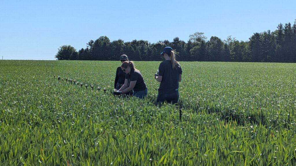
A series of four posts were positioned in the wheat, spaced 0.5 m apart and centred on the corresponding section of nozzles. The samplers were SpotOn water sensitive papers (WSP) mounted in custom holders to orient four papers at 90° to the sprayer: Advance (facing the sprayer), Left, Retreat (facing away from the sprayer) and Right.
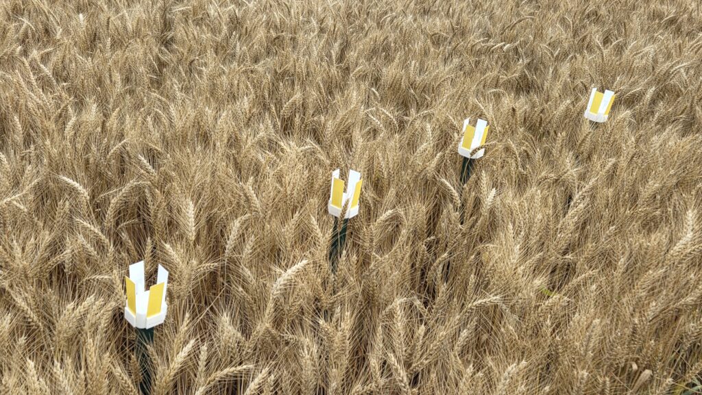
A parallel tramline approximately 1 m from the samplers provided access. The sprayer began spraying 15 m (50 feet) before the samplers and continued spraying the same distance beyond them. Once the spray settled, the samplers were retrieved. A single pass represented a repetition and there were three passes per treatment.
Papers were digitized using a DropScope (SprayX) and the analysis was performed in R (v. 4.6.0), leveraging the rpy2 library for integration with Python within the Colab environment.
What we saw
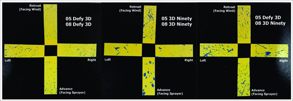
The following image shows a typical coverage pattern for each treatment. While WSP is not able to determine droplet size accurately, it can certainly reveal relative differences. It was clear that the Defy 3D produced smaller droplets than the 3D Ninety, and that there were far more of them. The hybrid condition shows a more heterogeneous coverage pattern, which would be expected given it represents a greater span of droplet sizes than either nozzle design used alone.
Defy 3D
3D Ninety
Hybrid Defy 3D and 3D Ninety
Continuing with general observations, we can average the coverage measured on each plane, on each sampler, for each treatment. When spoiled samplers were removed from the study (it happens), coverage can be described as either the area covered, or the number of deposits per area. With no exploration of variability, we see that the Defy 3D resulted in the greatest average coverage as represented by either metric.
| Treatment | n | Mean Area Covered (%) | Mean Deposits/cm² |
| Defy 3D | 46 | 3.73 | 126.35 |
| 3D Combo | 44 | 3.22 | 87.64 |
| 3D Ninety | 47 | 3.02 | 93.77 |
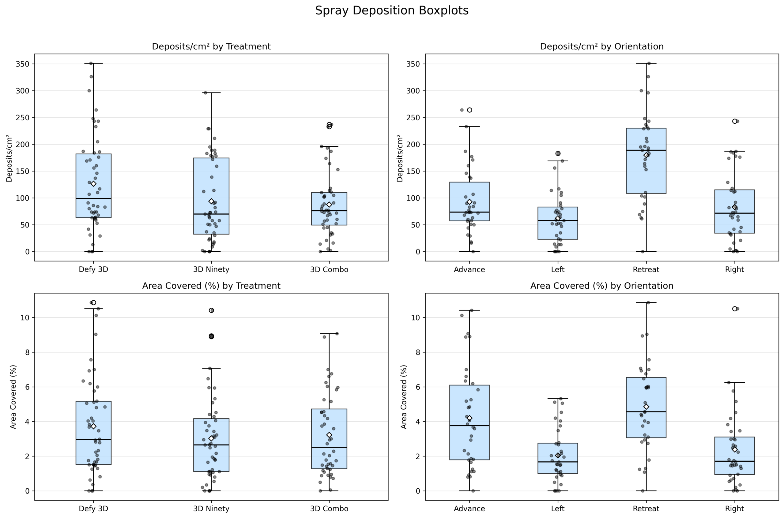
We can drill down and explore coverage by WSP orientation as well, this time including some measure of variability (standard deviation). As a matter of housekeeping, there was no evidence that repetition or post position had any meaningful bearing on coverage results (Pearson p of 0.422 and 0.455 and Spearman p of 0.267 and 0.217). We see the highest average number of deposits on the retreat side (facing the wind) in all treatments. Similarly, and excepting the combination treatment, we see the greatest average area covered on the same plane.
| Treatment | Orientation | n | Mean Deposits/cm² | SD | Mean Area Covered (%) | SD |
| 3D Combo | Advance | 11 | 83.00 | 53.58 | 4.98 | 2.80 |
| 3D Combo | Left | 11 | 63.36 | 38.07 | 1.67 | 1.24 |
| 3D Combo | Retreat | 10 | 138.20 | 58.38 | 4.12 | 1.93 |
| 3D Combo | Right | 12 | 72.00 | 63.84 | 2.29 | 1.93 |
| 3D Ninety | Advance | 11 | 67.82 | 52.92 | 3.41 | 3.38 |
| 3D Ninety | Left | 12 | 42.25 | 49.83 | 1.96 | 1.61 |
| 3D Ninety | Retreat | 12 | 191.17 | 54.20 | 4.89 | 2.07 |
| 3D Ninety | Right | 12 | 71.67 | 50.30 | 1.87 | 1.46 |
| Defy 3D | Advance | 12 | 124.92 | 65.48 | 4.19 | 2.64 |
| Defy 3D | Left | 12 | 80.75 | 49.75 | 2.48 | 1.74 |
| Defy 3D | Retreat | 10 | 207.70 | 115.84 | 5.55 | 3.45 |
| Defy 3D | Right | 12 | 105.58 | 75.92 | 2.98 | 2.83 |
We can illustrate this using box and whisker plots, which show all the data as well as the relative span of each treatment. This makes it easier to compare the treatments and determine if any differences in average coverage were significant or not.
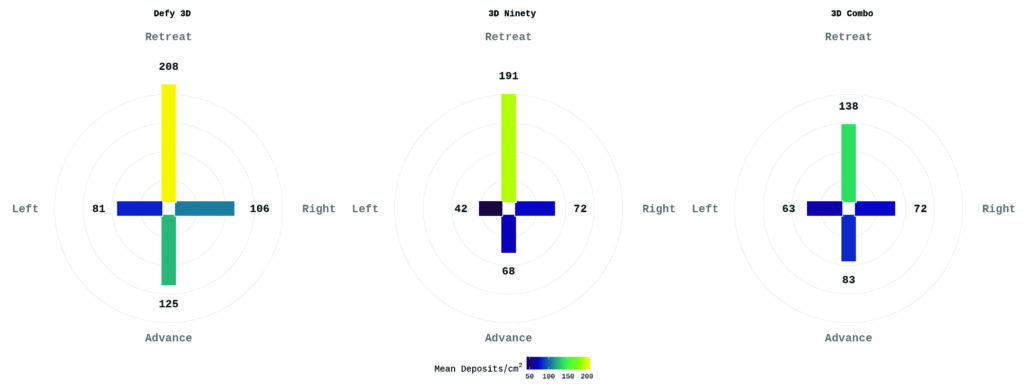
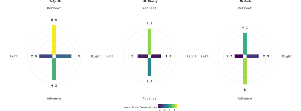
We can illustrate coverage in an even more intuitive manner using a rosette-style graph. Here we see the average deposit density or the percent area covered for each treatment on each plane. Note that the discrepancy between the Advance (shadowed by wind) and Retreat (wind-facing) side is far greater when the coverage is represented by droplet counts rather than area covered.
Interpretation and discussion
Deposits/cm² and percent area covered were strongly positively associated (r = 0.75), indicating that higher deposit counts generally corresponded to greater percent coverage. The relationship wasn’t perfect, suggesting that other factors also influenced coverage and leaving room for interpretation.
The Defy 3D produced the highest overall coverage, as reflected in total deposit counts. This is consistent with the fact that it emits a higher proportion of finer droplets relative to the 3D Ninety. While finer droplets can improve coverage, they are also more prone to drift and tend to deposit on the downwind face of vertical targets. We have evidence of this in all treatments, which showed more deposits on the Retreat (windward) face than on the Advance face, which was sheltered from the wind.
This deposition pattern is likely influenced by the rear-facing nozzle configuration (an ‘08), which delivers a higher application rate than the forward-facing nozzle (an ‘05). With higher boom heights or stronger wind conditions, this configuration may be less effective, as reported in previous studies. In this comparison, the Defy 3D also exhibited the greatest variability, suggesting greater sensitivity to such conditions.
The 3D Ninety and hybrid treatments were difficult to separate based on overall coverage. There was no significant difference in the magnitude of coverage between them, although the hybrid condition showed a more balanced distribution of deposits between the Advance and Retreat faces. In contrast, the 3D Ninety would be expected to produce a coarser spray that is less susceptible to deflection, assuming boom height is sufficiently low to maintain droplet trajectory. Despite this, it recorded more deposits on the Retreat face than the hybrid condition. We have no explanation.
The hybrid configuration was designed to improve deposition balance by combining complementary spray characteristics. The forward-facing nozzle produced finer droplets, which can be carried along by the sprayer’s forward momentum to enhance forward deposition. The rear-facing nozzle produced coarser droplets at a higher application rate, compensating for lower droplet numbers while counteracting forward momentum to improve retreat-side coverage.
Although the hybrid treatment appeared to provide a more even distribution of deposits between the Advance and Retreat faces, it is uncertain whether this would translate into improved biological efficacy. Further trials would be needed to evaluate whether this deposition balance leads to measurable yield gains.
It is also important to note that both the 3D Ninety and hybrid treatments were applied at 25.7 km/h (16 mph), nearly 20% faster than the Defy 3D treatments. This indicates potential for higher productivity. Given the relatively balanced deposition observed, a combination of a forward-facing Defy 3D nozzle and a rear 3D Ninety nozzle may offer improved resilience to changes in boom height and wind speed while maintaining adequate coverage at higher travel speeds.
Thanks to Clean Field Services for their participation in this study, thanks to Agflow Canada (Hypro / Shurflo) for donating the 3D Ninety’s, and thanks to Cesar Cappa, OMAFA weed specialist in horticulture for patiently explaining how to use R more effectively.