Tag: herbicide

Exploring the Accuracy of Drone-Applied Herbicide Treatments

Author’s note: Minor edits were made to this article on December 12, 2025. While the results remain unchanged, aspects of the interpretation have been adjusted upon reflection.

In 2024, Corteva conducted a study entitled “Drone-Delivered Herbicides: Comparing Lontrel^TM XC (Clopyralid) Efficacy Across Application Techniques and Water Volumes”. Go read all about it here. Their objective was to compare the relative efficacy of hand booms and drones, and to determine if drone efficacy was affected by low water rates. The researchers evaluated the area treated and the effective swath width by manually tracing the burned areas from an aerial NDVI image.

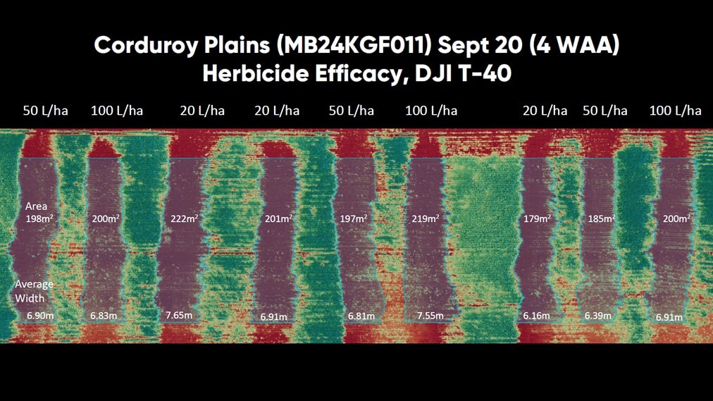
Interestingly, the study found that water volume had an insignificant impact on herbicide efficacy. But what really caught our attention was the inconsistent and variable shape of the treated area along each flight path (Figure 1).

Figure 1 – Image from work performed by Kevin Falk, Rory Degenhardt, Angela Fawcett and Neil Spomer, as presented at the 2025 Canadian Weed Science Society annual meeting in Vancouver, BC.

If the swath width fluctuates and vacillates along the flight path, then there is great potential for overlaps and misses throughout a treated area. Common practice is to rely on displacement (and drift) from upwind passes to deposit a sufficient cumulative dose of herbicide to mask areas of low coverage. This would be facilitated by consistent wind direction, higher altitudes, and a surface with little or no canopy to interfere with secondary deposition.

On the other hand, if the programmed swath width (i.e. route spacing) is too wide, and/or the the droplet size too large to permit sufficient displacement, then gaps in coverage would appear. And there is always the consideration of restricting the deposit to field boundaries and margins, particularly on the downwind side of the treatment area.

We explored these considerations by conducting a study that emulated aspects of Corteva’s work. We applied Roundup Transorb HC (a non-selective herbicide) instead of Lontrel (a selective herbicide specifically for broadleaf weeds). We used the DJI Agras T50 and the new T100 with two atomizers and a DJI RTK-2 base station, employing an array of operational settings. And, we flew multiple passes rather than a single pass for each treatment.

Part one of the study examined three programmed swath widths from both drones to compare their performances directly. Part two of the study evaluated the T100’s performance over a series of flight speeds and spray qualities. Burndown was evaluated using post-application orthomosaic images taken at 200 feet using a DJI M3M drone. Images were analyzed using Pix4D software.

Materials and Methods

Field Conditions

Applications took place in a 160-acre field of wheat stubble in Central Elgin, Ontario (42°45’29.3″N 81°05’58.9″W) on September 13, 2025.

Treatments

Each flight was centred on the right boundary of the treatment block, as indicated by a pin flag. Four passes were flown per treatment (i.e. two out-and-backs). There were no repetitions for treatments, so there was no need to randomize them.

Part One

The intent of this part of the study was to make a direct comparison of the swaths produced by the T50 and the T100. The T100 is heavier, has a larger volumetric capacity (100 L vs. 40 L) and is capable of faster flight (20 m/s or 64 km/h vs, 10 m/s or 23 km/h). We wrote about our first impressions of the T100, here.

Drone operational settings were selected to replicate those used in previous corn and wheat fungicide experiments with the T50. These settings are admittedly more restrictive (from the perspective of productivity) than those commonly used for herbicide applications. For example, and anecdotally, we have been told the T100 can spray a full section (~260 hectares or 640 acres) at 2.8 gpa and 20 m/s on one tank and one battery charge. However, we have no information about subsequent coverage, efficacy or off-target deposition.

Maintaining these operational settings allowed us to make a more direct comparison of herbicide vs. fungicide placement and efficacy. All applications were performed using a 250 µm spray quality (Table 1).

Treatment Code	RPAS	Programmed Swath (m)	Speed (m/s, km/h)	Altitude (m)	Volume (gpa)
A	Unsprayed	–	–	–	–
B	T50	6	6, 21.6	3	5
C	T50	8	6, 21.6	3	5
D	T50	10	6, 21.6	3	5
E	T50	6	10, 36	3	5
F	T50	8	10, 36	3	5
G	T50	10	8, 28.8*	3	5
H	T100	6	6, 21.6	3	5
I	T100	8	6, 21.6	3	5
J	T100	10	6, 21.6	3	5
K	T100	6	10, 36	3	5
L	T100	8	10, 36	3	5
M	T100	10	10, 36*	3	5

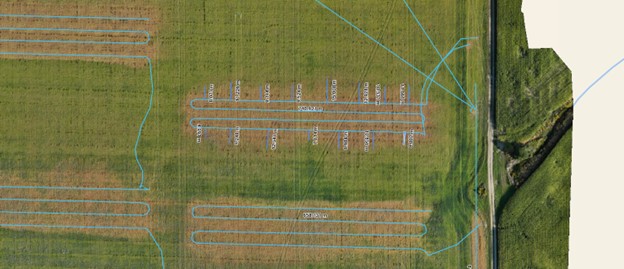
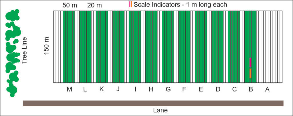
Table 1 – Part one: Drone settings. (*10 m/s was intended, but the T50’s pumps could not produce a 10 m swath at 5 gpa at that speed.)

Each treatment block was 150 m long, 50 m wide and a 20 m buffer was maintained between treatments (Figure 2). Two, 1 m scale indicators were placed in Treatment B to confirm scale during image analysis.

Part Two

The intent of this part of the study was to explore the new drone design and its capabilities. Particularly, the impact of high-speed flight on effective swath width, displacement and drift. The DJI controller advises an altitude of 5 m or higher (likely a safety consideration). We felt this was too high for consistent coverage, and compromised by flying at 4 m (Table 2).

Treatment Code	RPAS	Spray Quality (µm)	Speed (m/s, km/h)	Altitude (m)	Volume (gpa)
N	T100	500	18.3, 65.8^†	4	3
O	T100	250	18.3, 65.8^†	4	3
P	T100	80*	12.5, 45*	4	3
Q	T100	250	18.3, 65.8^†	4	3
R	T100	250	15, 54	4	3
S	T100	250	10, 72	4	3

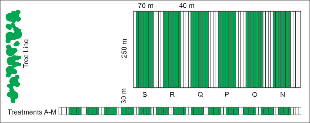
Table 2 – Part two: Drone settings (^†20 m/s was intended, but the drone only reached a maximum of 18.3 m/s before slowing as it approached the end of the treatment. *50 µm and 20 m/s was intended, but the T100 controller would not permit those settings, so a compromise was made.)

Given the greater potential for displacement and drift in this part of the study, we established wider and longer treatments blocks, and wider buffers between treatments. Each treatment was 250 m long, 70 m wide and a 40 m buffer was maintained between treatments (Figure 3).

Chemistry

The spray solution (PMRA research authorization 0054-RA-25) was premixed in a single batch. For part one, 80 L Roundup Transorb HC in 1,000 L water plus 0.05% Halt (defoamer). For part two, 700 L of the solution remained, so we added an additional 20 L of Roundup to approximately maintain the dose when dropping from 5 gpa to 3 gpa. This is a high dose of Roundup (~1.5 L/ac), selected to ensure that every drop that landed would create an obvious burn for easier analysis. It does, however, also mean that any reduced dose (i.e. striping) between passes would likely be masked. Drones were refilled after each treatment (to 40 L for T50 and to 65 L for T100) to negate any weight effect on the magnitude of the downwash.

Weather

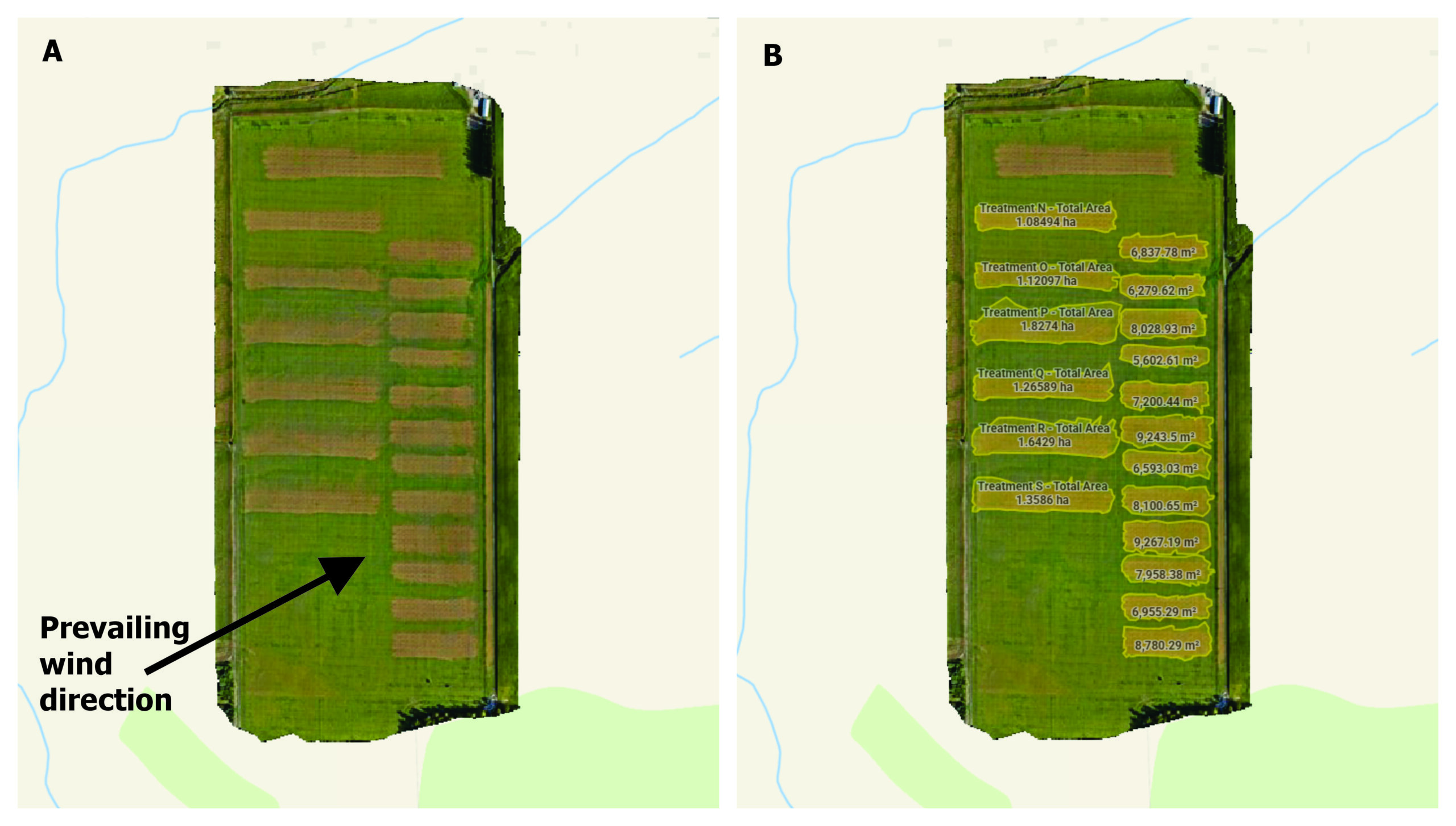
Weather data was collected using a Kestrel 3550AG weather meter (Kestrel Instruments) in a vane mount positioned 2.5 m above ground (Table 3). For part one, conditions were ideal: humid with a light wind in a consistent direction. For part two, afternoon wind speed increased, but predominant direction remained consistent (Figure 4A).

Time	Experiment Part	Treatment	Weather
10:05 – 10:58	1	B – G	18.6 ̊C, 78% RH, 0.0 km/h wind.
10:58 – 12:40	1	H – M	19.8 ̊C, 72% RH, 2.0 km/h wind.
12:40 – 1:50	2	N – S	22 ̊C, 61.2% RH, 7.0 km/h wind.

Table 3 – Treatment times and weather conditions

Figure 4 – Left (a): Prevailing wind direction overlaid on orthoscopic image. Right (b): Polygons representing manual traces of the perimeter of the burned treatment areas. Areas are noted for each treatment.

Estimating Effective Swath Width

The burned area indicates that the spray deposited met or exceeded an efficacious dose. This agronomic consideration of real-world efficacy sets the Effective Swath Width (ESW) apart from a swath width measured during calibration. Methods for calculating swath width utilize a sampling system aligned perpendicular to the flight path. Whether continuous or discreet samplers, this approach produces a coefficient of variation and some measure of over- and under-dose based on an assumed target threshold (dose or coverage). By measuring the biological effect (i.e. the burned area), we need not assume a target threshold – it’s indicated by the burn. Work with fungicides has demonstrated that the ESW can be a fraction of the measured swath width.

ESW was estimated using two methods, and while both approaches have inherent flaws, they still provide valuable information. A more realistic representation of ESW likely falls between the two.

In the first method, the perimeter of the area burned was traced to create a polygon (above, in Figure 4B). Then, the average width of that area was established from measured spans along the block. Finally, that average was divided by the four passes. Hereafter referred to as the “treatment width ÷ passes” method. This method produces an underestimate of ESW because each upwind drone pass can overlap and hide any displacement (and drift) from the previous. It divides the drift over however many passes are made.

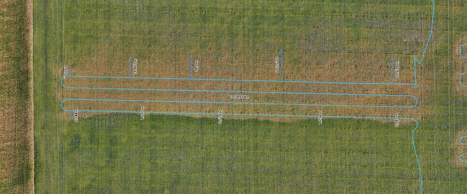
The second method overlays the flight path onto the area burned. The upwind side of the swath was determined from an average of at least five measurements along the upwind flight path. The downwind side of the swath was calculated the same way (Figure 5). Both the average upwind and downwind distances were added to arrive at the ESW. Hereafter referred to as the “port + starboard extent” method. This approach captures a clear representation of the upwind side of a single pass, but overestimates ESW by including any cumulative increase in drift from multiple passes on the downwind side.

Figure 5 – Example of port and starboard measurements along the downwind and upwind-most flight paths. The averages were calculated and added to estimate effective swath width.

Results – Part One

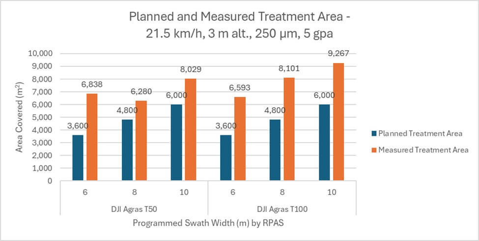
Planned versus Measured Treatment Area

The “programmed swath width” is something of a misnomer. More accurately, it is the route spacing and it describes the distance between passes over a target area. However, most drone manufacturers refer to this variable as programmed swath width, so that’s what we’ll do.

Planned treatment areas were calculated from distance flown × programmed swath width × number of passes. Measured treatment areas were calculated by tracing a polygon along the perimeter of the area burned. In all cases, actual was larger than planned by an average 36.1%. The T50 treated 32% more area than planned and the T100 treated 40% more area than planned, or 8% more than the T50 (Figure 6).

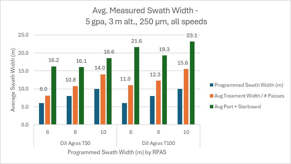
Figure 6 – Planned and Measured Swath Widths for T50 and T100.

Programmed and Effective Swath Widths

In all cases, the “treatment width ÷ passes” method produced an estimated ESW that was greater than, and positively correlated with, programmed swath width (Figure 7). For the T50, it was an average 26.8% wider. For the T100, it was an average 38.3% wider. The ESW calculated by the “port + starboard extent” method was larger still, but was not positively correlated with programmed swath width. For the T50, it was an average 52.8% wider. For the T100, it was an average 62.5% wider.

No matter the method used to estimate ESW, the T100 exceeded the planned swath width by more than the T50. Using the “port + starboard extent” method, the average T100 ESW was 21.3 m, which is an average 15.4% wider than the average 17 m ESW produced by the T50.

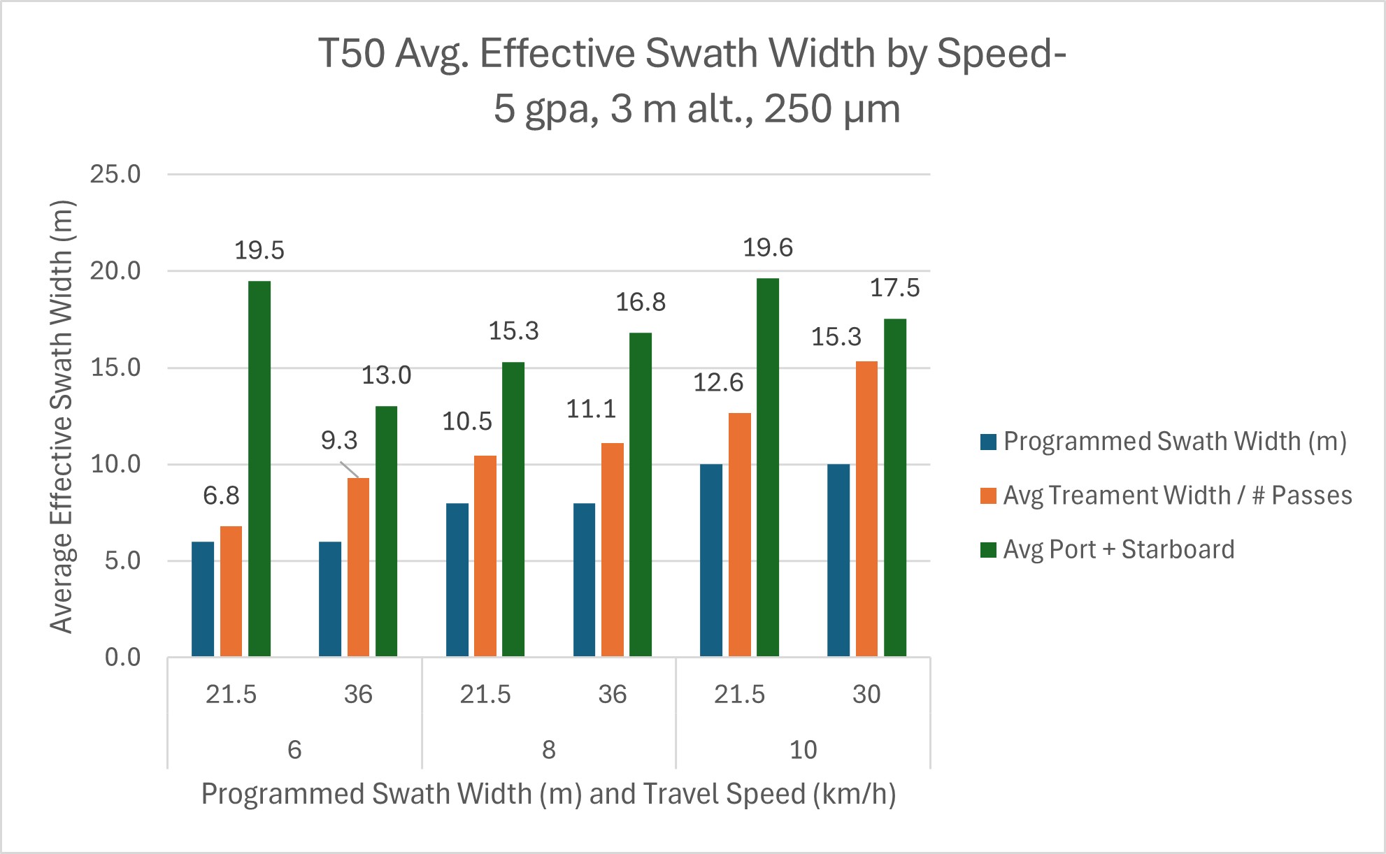
Figure 7 – Average measured swath width (two methods) compared to planned swath width for the T50 and T100 flown at 5 gpa, 3 m altitude, 250 µm spray quality and multiple speeds.

T50 ESW by Travel Speed

When travel speed becomes the independent variable for the T50, the “treatment width ÷ passes” method produces an average ESW that positively correlates with flight speed. At 21.5 km/h, the average ESW was 10 m, increasing to 11.9 at 30-36 km/h (Figure 8). This is typical and expected as higher speeds have been shown to produce wider swaths with the T10 and T50.

However, the relationship between speed and ESW is less clear when estimated using the “port + starboard extent” method. At 21.5 km/h the average swath was 18.2 m, but reduced to 15.8 km/h at 30-36 km/h (Figure 8).

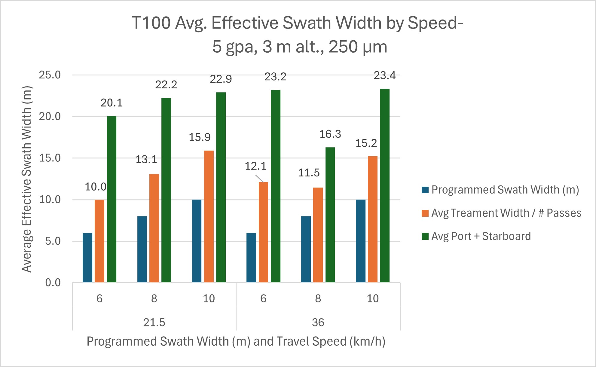
Figure 8 – Average measured swath width by speed for the T50.

T100 ESW by Travel Speed

When travel speed becomes the independent variable for the T100, neither method for estimating ESW show an effect from flight speed. The “treatment width ÷ passes” method produced an average ESW of 13 m at 21.5 km/h and 12.9 at 30-36 km/h (Figure 9). The “port + starboard extent” method produced an average ESW of 21.7 m at 21.5 km/h and 21 at 30-36 km/h.

Figure 9 – Average measured swath width by speed for the T100.

Results – Part Two

T100 ESW by Travel Speed

The effect of flight speed on treated area and ESW was examined. In each case, the treated area was significantly larger than the programmed area (Figure 10).

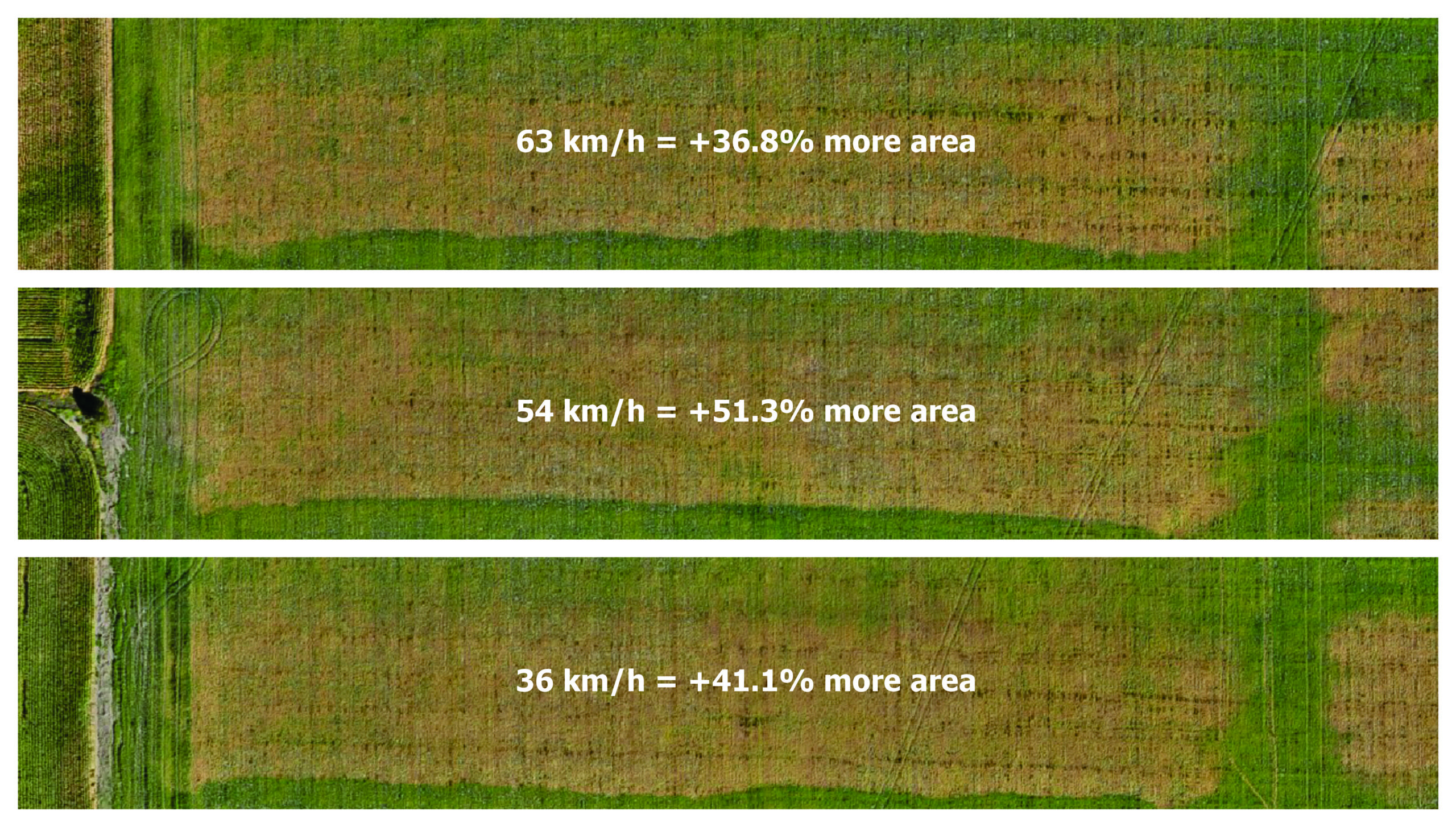
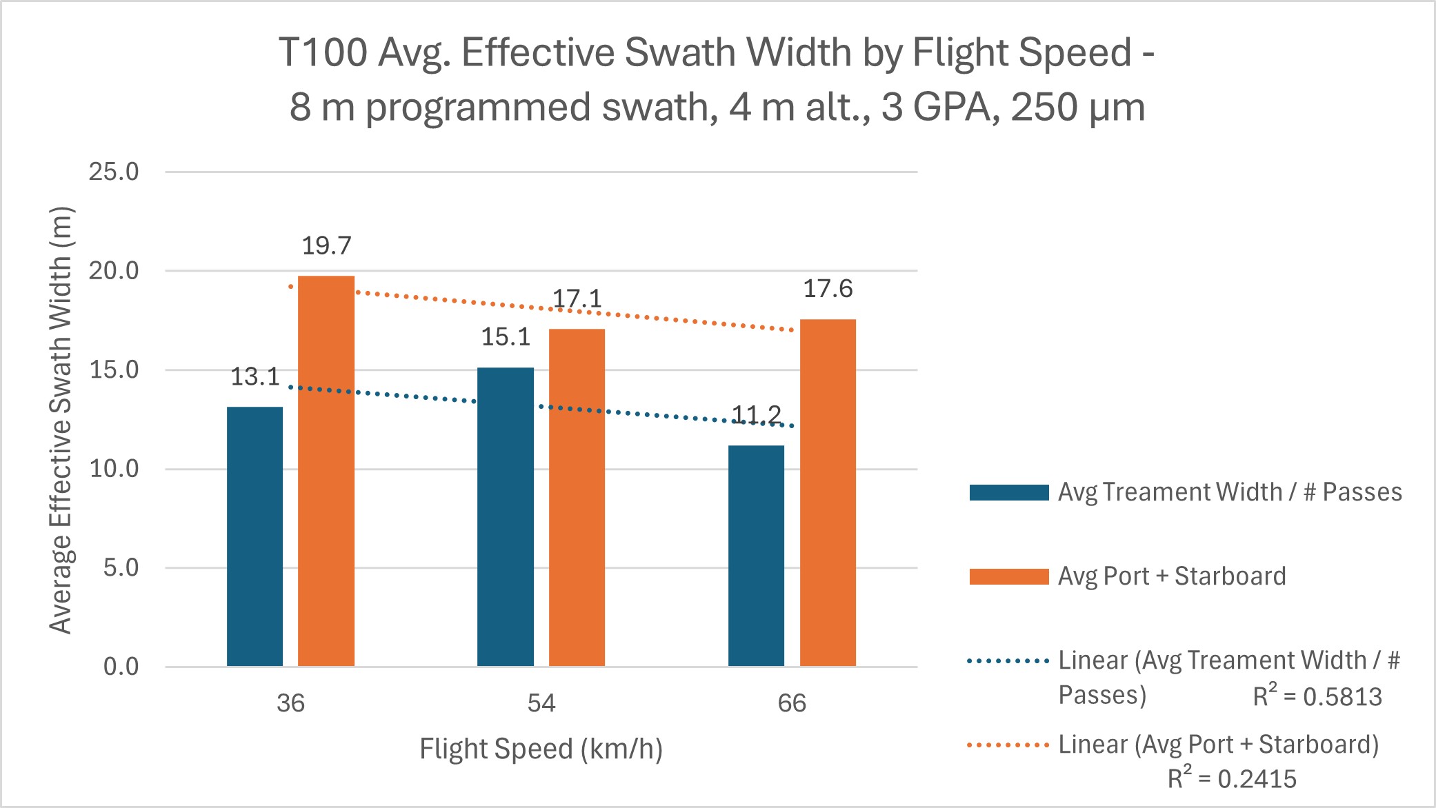
Figure 10 – Actual treatment areas compared to expected for the T100; three speeds.

Similar to Part one, travel speed did not appear to influence ESW in any consistent or significant way (Figure 11).

Figure 11 – Average swath width for T100 calculated using two methods at three speeds.

T100 ESW by Spray Quality

The effect of spray quality on treated area and ESW was examined. Once again, in each case, the treated area was significantly larger than the programmed area (Figure 12).

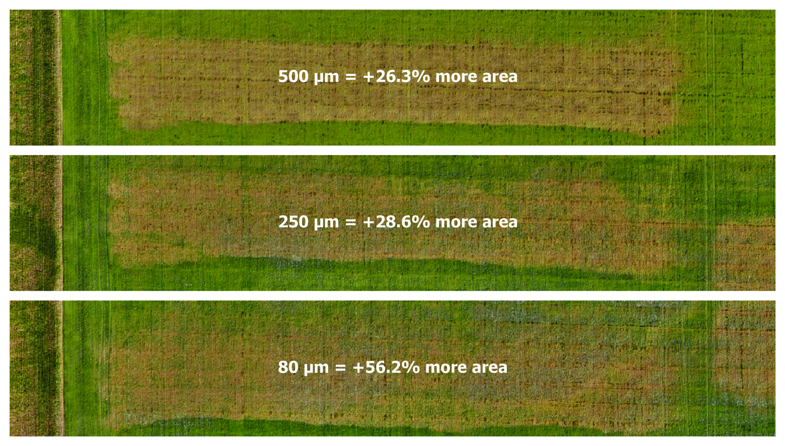
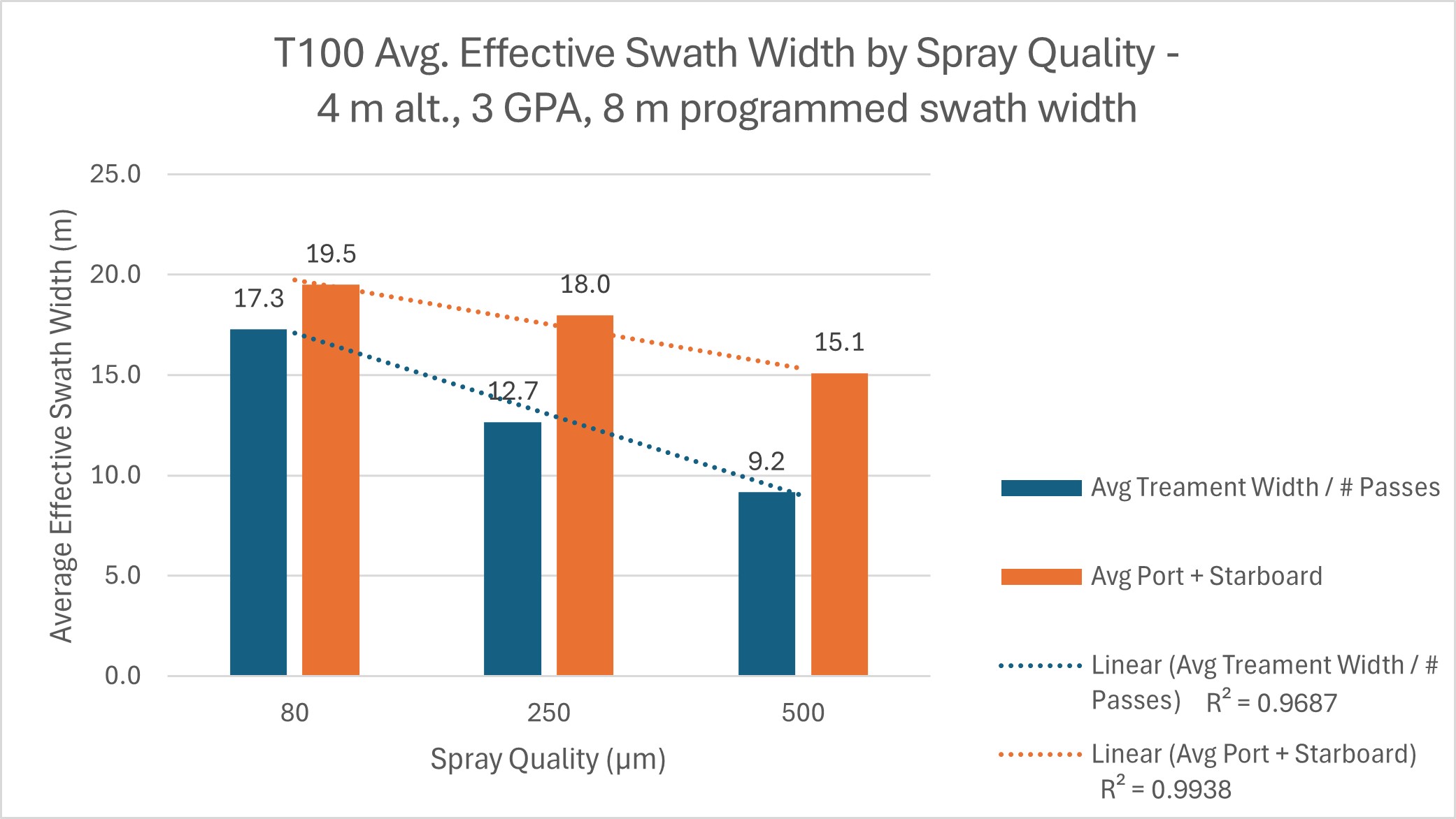
Figure 12 – Actual treatment areas compared to expected for the T100 using three spray qualities.

Effective swath widths estimated from both methods were negatively correlated with spray quality (Figure 13). Coarser droplets have greater mass, making them are less prone to displacement by wind than finer droplets. The “treatment width ÷ passes” saw an 80 µm spray quality produce an ESW 46.8% larger than a 500 µm spray quality. The “port + starboard extent” method saw an 80 µm spray quality produce an ESW 22.6% larger than a 500 µm spray quality.

Figure 13 – Average swath width for T100 calculated using two methods for three spray qualities.

Discussion

In all cases, the area treated (i.e. burned) exceeded the area planned. The T50 covered 32% more area while the T100 (with the same operational use case) covered 40% more. This implies that the T100 created wider swaths and/or drifted more than the T50.

The ESW estimated from herbicide efficacy appears to be considerably larger than those observed in fungicide efficacy / coverage studies. This is likely the result of the agronomic use case. Consider that herbicides have a relatively lower threshold dose than fungicides. Further, herbicide application on bare earth or into sparse canopies permits the lateral spread of droplets, where spraying fungicides into a dense canopy limits penetration in all directions. Even the sparsest coverage from a systemic herbicide produces a visual effect, and this binary result (i.e. hit or miss) extends the effective swath width. This should raise awareness of the importance of field boundaries and margins, particularly with herbicides.

When estimating ESW, the method used affected the results. The “port + starboard extent” method resulted in large and low-resolution estimations of ESW, whereas the “treatment width ÷ passes” method seemed to respond in a more predictable way, even if it underestimates the ESW. Ultimately, both methods produce rough estimates; they are not intended to replace traditional, quantifiable assessment methods. The “truth” is likely somewhere in between.

With that caveat reaffirmed, we assessed ESW using the “treatment width ÷ passes”. It was positively correlated with flight speed for the T50, as observed in previous work. However, this was not the case with the T100. Given that both drones were operated using the same settings, it is unclear why the T100 would produce such erratic results. Future work will evaluate T100 ESW using conventional methods.

When the T100 was flown using a span of three droplet sizes, there was a strong negative correlation between average droplet size and ESW. Once again, this aligned with previous experience. While rotary atomizers on drones tend to create smaller droplet sizes than reported by the flight controller, coarser droplets have greater mass, making them less prone to displacement by wind.

However, when the T100 was flown at at three speeds, the relationship with ESW was once again unclear. When flown at 36 km/h (~10 m/s) the T100 was flying at the top speed of the T50. It also flew at 54 km/h and at 66 km/h, which was the highest speed we could achieve at 5 gpa. The ESW (as estimated using the “treatment width ÷ passes” method) was essentially unchanged. While it is possible (and likely) that any increase in effective swath width due to travel speed was obscured by drift, pervious work has shown that drift increases concomitantly with speed. That does not appear to have happened here.

Perhaps this is a function of a greatly reduced dwell time diminishing the effect of the downwash. Or, perhaps, the T100’s capacity for higher speeds has allowed it to pass beyond translational lift into true forward flight, similar to a helicopter. Translational lift occurs any time there is relative airflow over the rotor disk. As headwind and/or forward speed increase, translational lift increases, resulting in less power required to hover. According to Transport Canada, it is present with any horizontal flow of air across the rotor but most noticeable when the airspeed reaches 16 to 24 knots flight (8.25 to 12.8 m/s or 30 km/h to 46 km/h). This would greatly reduce the effect of the downwash on droplet movement. In our first impressions of the T100, we found that flying slower overheated the battery. This did not occur at higher speeds, and this efficiency supports the premise that it moved past translational lift, perhaps achieving true forward flight.

If this theory is correct, it’s a new development for rotary drones, which were not previously capable of reaching these speeds. Downwash was an unavoidable side effect of the flight, but may now be a tool for the operator to use as the situation warrants – battery temperature notwithstanding. Perhaps it warrants a return to horizontal booms positioned beyond the downwash in order to improve coverage uniformity. On the other hand, we saw that it took the T100 roughly 100 m to reach the target 66 km/h, meaning it moved from hover to translational flight and beyond over that distance. This raises questions about how they spray would respond throughout that transition.

More work is required.

Acknowledgements

Adrian Rivard and Stuart Hunter (Drone Spray Canada), Adam Pfeffer (Bayer Canada) and Mike Cowbrough (Ontario Ministry of Agriculture, Food and Agribusiness) are gratefully acknowledged for their participation, and both in kind and financial support of this study. Thanks also to Mark Ledebuhr and Tom Wolf for discussions surrounding the interpretation of these results.

November 4, 2025

A Strange Case of Herbicide Injury in Grape
In the summer of 2024, six Ontario vineyards participated in an authorized herbicide trial. The objective was to assess efficacy as well as determine if the product fit the timing for seasonal weed and sucker management. If successful, it could replace the expensive and time-consuming manual labour required to remove suckers.
Each vineyard applied the same rate, at similar times, employing optimal sprayer settings. A few weeks after application, the researchers and registrant toured the vineyards. They were pleased with how quickly and effectively the product worked on both targets at all six locations. However, one vineyard reported visual injury on a sloped region of their operation.
This raised two questions:
1. Assuming the cause was drift, and not direct overspray, why did it only happen in a specific region of a single vineyard?
2. Whether drift or overspray, what is the potential for the applied rate to cause injury?
The vineyard manager and sprayer operator investigated the application equipment and found no problems with how the sprayer was calibrated or operated. Further, the nearby weather stations recorded reasonable environmental conditions. So, that seemed to discount accidental overspray and wind-borne drift.
Then we considered the topography. The level portion of the vineyard appeared undamaged, but as it began to slope downhill, we saw damage on leaves and shoots in the bottom half of the canopy. It was almost as if a stratum of herbicide stayed level as the ground fell away. We discussed temperature inversions, volatility, and sprayer wake, but nothing fit.
Then we stepped back and found ourselves looking up at the Niagara Escarpment. The Escarpment is a long cliff formed by erosion, separating the higher, level ground from where we stood below. And then we had an idea: Could the product have been lifted into contact with the canopy by a Katabatic wind?
The theory
On clear nights with calm winds, the ground cools rapidly. Air in contact with the colder ground cools by conducting heat to the ground and by radiating upwards. When this cooling process occurs along mountain slopes, or on top of a plateau, the cooling air becomes colder and denser, causing it flow downslope like water. Perhaps a layer of relatively cool Katabatic wind off the escarpment slid under the warmer layer of air in the downslope portion of the vineyard. And, perhaps, any product still suspended in the air was lifted upwards into contact with the grape canopy.
Cold air (blue) slides under a warmer layer of air (orange) that carries traces of herbicide in the form of Very Fine, suspended droplets. It is lifted into contact with the lower portions of the grape panels.
Even the coarsest hydraulic nozzle produces a population of driftable fines. These fines take a long time to fall, and some are essentially buoyant. In the following histograms, we see actual data from a nozzle rated between Medium and Coarse. The operators actually used an air-induction nozzle with a much coarser spray quality, but we’re using this data set as a worst-case scenario example. If we divide the volume produced into its constituent droplet sizes, we see that most of the volume is comprised of droplets between 150 and 250 microns.
However, droplet diameter shares a cubic relationship with volume. If we plot that same volume by number of droplets, we see the majority are between 18 and 74 microns in diameter. These very small droplets would fall so slowly that any atmospheric disturbance would displace them. Depending on the crop’s sensitivity to the herbicide, they might carry sufficient active ingredient to cause injury, assuming they didn’t evaporate to the point that they were no longer biologically active.
There are a lot of assumptions in this theory, and perhaps it’s far fetched, but it was the best we could figure. So, if those droplets were lifted into contact with the canopy, were they capable of causing injury? To find out, we conducted a simple, non-replicated bioassay.
The bioassay
On the morning of July 12, we filled a spray bottle with 50% of the field-rate (including 1% v/v MSO) and set the nozzle to the finest setting. We applied a single spritz about mid-way up the canopy of the same Riesling grapes on a VSP flat cane training system. We did this on the upwind side on both older (lower canopy) and newer growth (upper canopy). Then we performed a series of serial dilutions, halving the concentration each time, and repeating the application.
Our hope was to see a subtle response curve when we plotted concentration against tissue damage. Perhaps we’d even see a different curve for older versus newer tissue.
The vineyard manager photographed and recorded observations on an approximately weekly schedule, with a gap in observations between weeks three and six. The following images show the results of a ½ dose treatment, and a 1/16 dose treatment tracked during that period.
The results
We observed the following:
- Fruit, foliage, and shoots were injured at all doses by three days after application.
- Initial injury remained stable; no secondary injury was observed.
- The degree of injury at the lowest dose was significantly more severe than the injury observed following the original May 31st application.
- Regular vineyard operations, such as mechanical leaf removal in the fruiting zone and hedging, removed some of the damaged leaves and shoots.
- The study did not include an assessment of harvest quality.
This was severe injury, even at the lowest rate. When compared to another herbicide commonly used for perennial weed control (e.g. Ignite SN – glufosinate ammonium) the injury we saw manifested very quickly.
Recently, researchers at Cornell have been exploring the herbicide we used in this study in perennial weed and sucker control in apple orchards. They did not experience any drift issues and found it to be effective between 90-180 ml/ha (0.5-1 oz/ac) (personal communication). That’s ~4x less than the rate proposed for registration in Canada, and it suggests the herbicide in question was certainly capable of causing the damage at very low concentrations.
Ultimately, we can’t be certain how the initial off-target damage occurred, but we were able to evaluate damage potential using a rough-and-simple bioassay that any grower can try. In unusual cases of drift it’s important to know if the product we suspect is even capable of causing the damage. A simple evaluation using serial dilution and a squirt bottle can tell us if we need to look more closely, or look somewhere else to explain injury.
Thanks to Kristen Obeid, OMAFA Weed Specialist (Horticulture) and Josh Aitken, Vineyard Manager of Cave Spring Vineyard for their contributions to this work.
March 7, 2025
Pre Emerge Spraying with a Custom Applicator: Drive-Along Diaries #3
It was May 16th, and I was standing at the front counter of Clean Field Services (CFS) in Drayton, Ontario, looking forward to an interesting day in the buddy seat. While I was waiting on the sprayer operator to check and fill the sprayer, I asked Todd Frey, Customer Service Rep, to give me some background into the company.
Clean Field Services
Todd’s father, Dennis, started spraying for a neighbour in the 1990s using a truck-mounted skid sprayer. In 2003 he began offering custom application services from their Drayton location, and in 2009 incorporated as CFS. Primarily offering contract application services to small fields (<20 acres), they also offered scouting and agronomy services, sold seed, and created nutrient management plans.
A big part of the business is liquid fertilizer. Many local retailers are set up to apply dry fertilizers, but here they pre-blend liquid fertilizer and can fill a sprayer in three minutes thanks to their new John Blue, 20 hp pump with it’s 4” inlet. More on tendering, later.
Scheduling
Todd explained that today would be all about pre-plant herbicides in soybean and corn. The farmer tills, then CFS sprays, then the farmer tills again to incorporate the herbicide before planting.
Much of the scheduling is arranged over the previous winter, but plans had to be flexible to accommodate changeable weather. Case in point, there were originally six jobs scheduled for today, but two were added at 6 am when clients called to ask for last-minute service. The wet spring was keeping farmers off their fields, so planting pressure was mounting, and sprayer scheduling had been particularly tough. Todd tells people “We’re not 911 dispatch!”, but ultimately does his best to accommodate the short notice.
That’s when Brendan Bishop came in to collect me. This was Brendan’s second year as an operator having started in 2023 as a tender truck driver and “graduating” mid-season to spraying. As I followed him out, I wondered how he’d stack up compared to the older, more experienced operators I’d worked with. Spoiler: Brendan had skills.
The Sprayers
CFS owns a John Deere 410R and a 4038. They also have an operator on retainer who owns his own 4030. CFS used Rogator in the past and Apache before that. The Rogators featured a lot of flow capacity, making them great for spraying 28%. CFS switched to Deere for the service and to take advantage of a few technologies I’ll describe shortly, and now they can stream liquid fertilizer at rates as high as 46 gpa at 14 mph.
Today, we’d be in the 410R, which featured pulse width modulation (PWM) and boom recirculation. I was told that customers appreciated the optics of not wasting up to 40 gallons on priming. But the sprayer also featured direct injection from four, 50 gallon tanks, and that puzzled me. Why would a sprayer have two seemingly incompatible features? No one would inject product just prior to the manifold and then circulate it right back to contaminate the tank.
Brendan agreed that they were mutually exclusive, but both had roles in minimizing waste and downtime from priming, rinsing, and custom spray mixes. For example, an early pass over corn might have Marksman and Armezon PRO in the tank, and then Roundup could be direct injected at rates specific to the weed pressure. On the other hand, if he didn’t need direct inject for custom mixes, he could utilize recirculation to avoid priming.
The sprayer automatically disengaged recirculation when direct injection was operating. That restriction could be over-ridden, but you couldn’t run them both by accident. Nevertheless, his policy was to always take a breath before engaging either system because a mistake might be irreversible and require a purge and refill.
8:30
We left the yard and cruised down country roads at 40 mph until we hit the more populated regions. This part of Ontario had a lot of Mennonite residents, and their horse-drawn carriages required a wide berth. That got particularly tricky on narrow roads and single-lane bridges, but Brendan was patient and obviously practiced.
We arrived at our first field at 8:50. We parked at the edge and started unfolding the boom as Brendan called dispatch on the cab radio. The field was 15 acres of Roundup ready corn, and we’d be spraying a pre emerge herbicide in 28% UAN at a rate of 20 gpa. We knew all this before we ever left the yard thanks to CFS’s operations management system.
The AgLogic Operations Management System electronically assigns work orders (e.g. chemistry, field location, field boundaries) to the equipment, allowing dispatch to track, schedule and route their assets. It also pushes weather information and any special notes to the operator. The AgLogic tablet and the John Deere monitor are supposed to be compatible with one another, and it was generally slick, but there were a few glitches.
AgLogic and the Job Centre monitors showing how the boundaries were different for the same field. The operator has to make a commonsense call.
Dennis was on dispatch, and Brendan asked if he should send for Simon, their tender truck operator. He was going to need water for the next job and had planned this job to end as empty as possible. Dennis agreed to send him as Brendan noticed aloud how rough the ground was – this field had only just been plowed. Dennis said they’d had to wait for the farmer to plow and warned Brendan of a particularly bad patch that he was familiar with. Brendan signed off and smiled as he warned me to hold on tight. Then he hit start on the AgLogic work order, and we were off.
He wasn’t joking – this ride would have qualified as a theme park roller coaster. I’m sure I left hand and face prints all over his windshield. He had to turn off boom track and go manual and had to cut a second headland. It was hard to hold the rate steady because our 4 mph speed dropped the PWM to the minimum 25 PSI and the duty cycle was maxed out.
Eventually we got up to a roaring 7.7 mph and by 9:25 we were done with less than two gallons left in the tank. While I searched for my kidneys, Brendan entered the summary into AgLogic: 19.65 gpa. He added a few choice comments to the file and in less than a minute he was done. CFS now had the information for billing with no hardcover book for the operator to mess up and no bad penmanship to decipher. As I said, slick. Have a look at a field ticket, here.
9:30
We waited in the client’s yards for Simon. Brendan said he’d fill wherever he needed to; on the shoulder of the road or slinging the hose across a ditch into the field. But a client’s yard was always safer and therefore preferred. It was worth waiting.
According to the work order, the next job was 15 acres of Roundup burndown at 12.5 gpa, so Brendan was doing the math on how much water he’d need (plus one acre’s worth for buffer). Simon showed up at 9:42 and we were loaded by 9:45. Just before we hit the road Brendan called dispatch to ask where to send Simon next. Efficiency takes planning.
9:54
We parked at the field entry and Brendan engaged the recirculation to push the remaining UAN and pre-emerge in the lines back to the tank to dilute them. Then he turned it off, engaged the direct injection of Roundup, and started priming the boom. This sprayer featured Auto Boom Prime: The operator set a target displacement volume (in this case, 40 gallons) and when the flow meter reached that value, you were primed.
As we waited Brendan explained that we weren’t doing anything today that couldn’t handle a little Roundup, so even if it somehow did circulate back to the tank, it was no big deal. He started the work order log at 10:02 checked for any warnings associated with the field before we were off again.
This was a narrow field. So narrow that we would likely overlap in the middle just from spraying the boundary. Brendan drove that first side manually, cleaning up the corners and margins while skillfully dodging fenceposts as best he could. Nevertheless, we tested the breakaway section a few times. He was nonplussed and said that any operator claiming they’ve never nicked a tree or a fencepost is either too far away or lying.
I asked why he didn’t use fencerow nozzles with Roundup and he gave two good reasons: 1. If you succeed in burning out all the grasses, broadleaf weeds like burdock move in and cause new problems. 2. Overspray was too risky when the target field abuts another crop.
Regarding his second point, I saw what he meant as we turned to spray the rest of the boundary, right next to winter wheat. On the back of the joystick are the secondary controls, which Brendan used to nudge the boom a few inches left or right along A-B line, constantly adjusting for the wheat.
At 10:17 he closed the work order, which digitally winged its way back to CFS for accounting. We folded up and followed behind as we headed back to the yard for a refill. Going back made more sense than tendering since the yard was en route to the next job.
Tendering
CFS fills their 20,000 gallon holding tanks from their own well, which is 300 feet deep and rated at 4,000 gallons per hour. Instead of installing more holding tanks, they doubled the floats to half the refill time. In addition, they have a tractor-with-wagon tender system with a 4,000 gallon capacity (and four serial induction bowls). Their transport truck is strictly for carrier and has two, 4,000 gallon tanks. In total, they can have 32,000 gallons of water on hand.
They recently improved their transfer pumps to keep up with so many small acreage jobs. It used to take up to 25 minutes to fill a 4,000 gallon trailer. Now they can pump up to 480 gpm through 4” lines and fill that same trailer in less than 10 minutes. And they have two such fill systems so no one has to wait their turn.
Their efficiencies are now found in the logistics of planning jobs that avoid rinses and minimize sprayer travel time where possible. The company isn’t afraid of road miles, preferring to drive further between jobs to avoid having to clean out the sprayer. Floating the sprayer to save engine hours didn’t made economic sense for them since you needed a wide-load permit, time to un/load the sprayer and you couldn’t transport at night.

It wasn’t “Gone in 60 Seconds” but we weren’t there much longer than that.
10:57
The next job was an L-shaped field. Brendan noted that weird field shapes were par for the course. As we drove, he said that some fields were so tight that he had to fold the booms almost completely to fit while spraying. He said he’d sprayed fields that no 120’ boom had any business being in. He’d had sideview mirrors pushed against the cab and was happy the Deere plumbing wasn’t on the outside of the folded booms, because he’d been snagged by branches in other sprayers.
Speaking of the boom, he was using LDM 08 nozzles, and the height was set to 30”. He would have liked a lower boom, but it wasn’t realistic on these rough and rolling fields. This field was short and sweet, and we were soon headed out.
11:10
This field was 19 acres and once again I saw it was narrow, meaning a lot of manual spraying on the boundary and very little autosteer in the middle. Brendan scanned back and forth between the boom end, the monitor, and ahead of the sprayer as we drove along at 7.5 mph.

When I mentioned the lack of autosteer he said he didn’t get to use it as often as I might think. Many of the corn fields he sprayed were planted by farmers with no GPS, so while he did use the A-B lines, they were mainly to alert him to turns. The actual steering was manual as he followed the planting lines.
I should mention that Brendan established a new boundary for every field, even through AgLogic provided one. He elected to establish this new boundary because once he sprayed the perimeter the monitor could tell him exactly how much area was left to spray. So, he would spray the boundary, check the area remining, and use his cell phone to calculate the differential between the volume in the sprayer and the target rate. He did this now to ensure he had enough water for the last four acres. He wanted to end empty because he would be switching back to 28% UAN next. Based on his math, he pushed the rate to 20.5 gpa to use up the water.
These rate changes would be difficult (perhaps impossible) to achieve without PWM because it would be based on pressure changes, and not duty cycle. It might even require switching nozzles. This is also when direct inject shines as it could maintain the Roundup rate independent of the carrier rate. Brendan said that fields were somehow always bigger than expected, so he was a big fan of the flexibility these features afforded him.
11:28
Now we’re back in the yard to fill with 28% UAN. Brendan was planning on a six acre corn field in the Township of Southgate, which was about a 45 minute drive, so we had to fill precisely.
We arrived at 12:27 and had to ask the client where the field was on the property. Surprise! The client wanted us to do eight acres, or 25% more than we’d anticipated. There was no way we could stretch the load that far, so Brendan told him we’d drive all eight at a reduced rate and make up the remaining nitrogen later when he came back with drops. We adjusted the rate from 28.75 gpa UAN to 22.6 gpa and at 12:46 we were done spraying, and the job submitted.
12:51
Simon is back with water and Integrity for our next job in pre-emerge corn, which is why Brendan wanted to be empty of 28% UAN. By 1:02 we were full and headed to a 32 acre job spread over two fields. Brendan chose to do the smaller, four acre field first so if he had to make any rate changes in the second field, he could spread a smaller difference over more area. Clever.
But where was this little field? Turned out, it required us to drive through a swamp, flushing two ducks and a deer in the process. As if that wasn’t bad enough, we both started to laugh when we saw the field. The ground must have been plowed 10 minutes before we arrived because it looked like an earthquake had hit it.

There’s a good reason you don’t spray freshly plowed fields. Once again, I did my pinball impression and idly wondered if Deere didn’t install seat belts in the buddy seat because they were trying to dissuade people from using it. Even Brendan bounced around despite the air ride driver’s seat.
We were relieved that the larger of the two fields was a breeze. Brendan did his math trick and elected to nudge the 16.1 gpa up to 16.7 in order to end empty. By 1:45 we were off for our last tender of the day.
1:50
The last three jobs totaled 70 acres and required a single fill. We were moving into Roundup-ready soybean, so we’d be spraying Roundup Transorb HC (glyphosate) + Tavium (S-metolachlor and dicamba). Brendan said they’d clean the sprayer thoroughly afterwards if they had to, but it was preferable to schedule a series of corn fields for tomorrow because they wouldn’t be bothered by dicamba residue.
We met the tender wagon and Brendan and Simon started loading Tavium into the inductor bowls for transfer to the sprayer. Then Brendan hosed down each bowl to rinse them and transfer that rinsate into the sprayer as well. Afterwards Brendan used the inductor bowl on the side of the sprayer to rinse the jugs because he felt the water pressure was higher on the sprayer and did a better job of cleaning them out.
2:35
This was a 11.75 acre field, and it should have been simple… but it seemed nothing was. The work order map showed the digital boundary, but the actual plowed field was much larger. So, it was one continuous field and we were supposed to spray only part of it. Where exactly was the boundary?
Eventually Brendan spotted some unsprayed grass that hinted at where other equipment had driven in the past. That subtle visual cue would have been impossible for an operator to see in the dark.
As we positioned ourselves to start spraying we saw the note on the work order to “mind the garden”. Garden? What garden!?
Eventually “Eagle-eye” Brendan spotted a couple rusty, foot-long lengths of rebar hammered into the soil along the edge of the field. They were perfectly camouflaged to match the colour of the tilled earth, hungry to puncture the tires of the unsuspecting, and doing a very poor job of indicating a “garden”. Once finished, we primed the boom (40 gallons) on the field margin to have it ready for the next job.
3:05
According to the work order, this 37 acre job warned us of yet another small garden. This garden was emerged, making it easier to find, but also making it a nerve-wracking off-target risk. So, we literally steered clear of it, leaving a wide berth.
That didn’t stop the woman who was tending the garden from marching purposely out to sprayer to get Brendan’s attention. He stopped and braced himself as he climbed down to speak to her. We both expected he’d get an earful for spraying around those vegetables. After a brief exchange he climbed back into the cab and smiled. She didn’t chew him out – she chastised him for not getting close enough! You can’t win.
4:05
The last field was 20.5 acres. It was flat, square and promised to be a straight-forward end to a complicated day. We drove 9.6 mph on the headland and just as we were finishing the circuit, we saw tilled earth outside the boundary indicated on the monitor. Wait – is that bit planted, too? Are we supposed to spray that as well?
Brendan guessed it was an additional three acres. He’d asked Simon to load an extra acre’s worth of spray mix when we loaded, and I now understood why. He did some quick math and said we’d have enough if we dropped the rate a bit.
We coasted back and forth over the field, watching the remaining volume drop on the monitor, hoping we’d make it. We considered adding rinse water to the tank to thin the concentration. That would give us enough volume, but we’d be diluting the chemistry too much. Then we figured if we had to we could empty the tank just to the point of starving the pump, add water from the rinse tank and push the ~40 gallons left in the lines from behind.
The tiny, unsprayed strip caused the PWM to flutter between one and three nozzles on that last pass. Neither of us realized we were holding our breath as we watched the spray volume drain away on the monitor.
And then we were done! It was a photo finish and we both let out an explosive gasp as we started breathing again. It was such a narrow victory that we climbed out to look in the tank, and I’m here to tell you, it simply does not get any closer than this. We bragged like successful hunters all the way back to the yard and told anyone that would listen when we arrived at 5:00.
As I packed to leave, Brendan asked Dennis if he had to go clean out the sprayer. Dennis said a little dicamba would help tomorrow morning’s pre-emerge applications, so no. But he smiled as he warned “Although, betcha someone will call in at 6 am to ask for IP beans first.” Driving home, thankful for my comfortable car seat, I wondered if they would.
Take Homes
- Planning ahead is always good advice. However for a custom applicator, it’s absolutely critical. The goal is to be efficient and effective with as little risk as possible, and you can’t accomplish that unless you know where you’re going, when you’re going there and what to expect when you arrive; and not just the immediate job but minimum three jobs ahead. When time, manpower and consumables equal money lost, the stakes are high to have a solid strategy before you leave the yard.
- Then again, rigid planning can be A BIG MISTAKE… unless it includes planning for the unexpected. Almost without exception, these fields were not as advertised. Most were larger than anticipated, so knowing how to stretch a load (e.g. dilution, changing rates, carrying a little extra, using clean water to push spray mix from behind) meant we could roll with the punches without leftovers or deficits. One strategy was to spray smaller fields first, so larger remaining fields could absorb a smaller, distributed differential. Another was to spray the headlands, calculate the remaining area, then determine a rate that fits the remaining volume in the sprayer. This all assumes you performed some solid sprayer math when you loaded, of course.
- Autosteer, while awesome, was not used near as much as I expected. Small, irregularly-shaped fields that were recently ploughed, abutting sensitive crops and land-mined with “no spray” gardens meant manual headlands (maybe two) and slow speeds. And when the client doesn’t use GPS to plant, you don’t use it to spray except to alert you to turns. Anyone that thinks the operator can be replaced by automation should ride along in these conditions. There are lots of situations where we still need grey-matter and experience behind the wheel.
June 12, 2024