Category: Featured Article

Articles that are featured on the homepage

  • What is Spray Quality, Part 2 – Describing Sprays

    What is Spray Quality, Part 2 – Describing Sprays

    Hydraulic atomizers comprise the majority of agricultural nozzles. They work by forcing a liquid through an orifice, resulting in a liquid sheet that is inherently unstable. The sheet breaks into ligaments and eventually droplets within a few centimetres of leaving the nozzle. The physico-chemical properties (elongational viscosity, dynamic surface tension, etc.) of the liquid affect the shape of the sheet and its stability, and therefore play a role in atomization.

    The dimensions of the liquid sheet depend on the nozzle type and the conditions in which they release the liquid. Flat fan nozzles, the most common in agriculture, force the liquid through an elliptical orifice that results in a sheet that is thicker in the middle and tapers at the edges. Nozzles that produce wider fan angles have narrower orifices, creating thinner sheets that ultimately produce finer sprays. Higher flow rate nozzles produce thicker sheets. A deflector nozzle impinges a stream of liquid against a plate that forces the stream flat and spreads it out, creating a different set of forces that destabilize the sheet. A cone nozzle generates a swirling action that results in a less stable sheet.
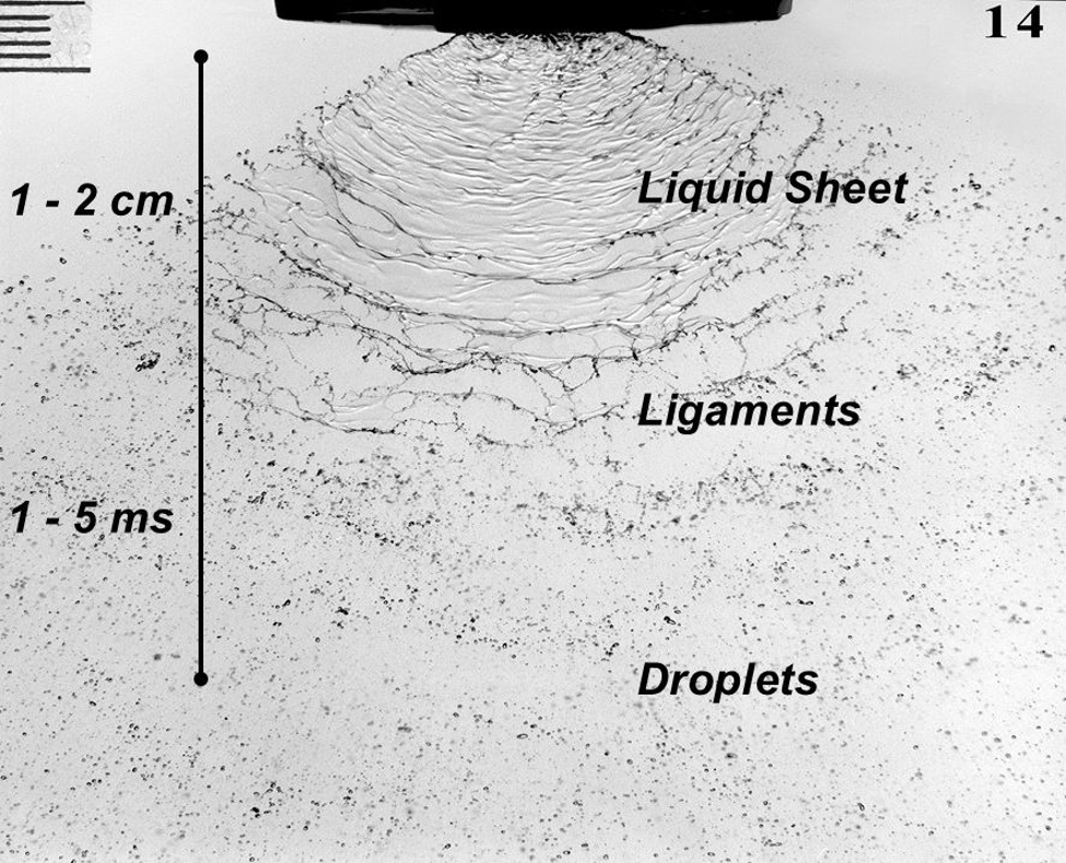
    Fig. 1: Three stages of hydraulic atomization of a flat fan nozzle. A sheet emerges from the exit orifice, which becomes unstable, forming ligaments that ultimately break into droplets (Image Source believed to be Silsoe Research Institute)

    If we place these nozzles into an airstream, either from travel speed or ambient wind, the spray sheet will become less stable and result in finer sprays. The amount of air-shear atomization will depend on the relative orientation of the nozzle sheet and the moving air. Nozzles that spray parallel to moving air produce less air shear and therefore result in coarser sprays than nozzles oriented perpendicular to the air stream. This characteristic is exploited by aircraft as a means of droplet size control, having a greater effect than spray pressure. 

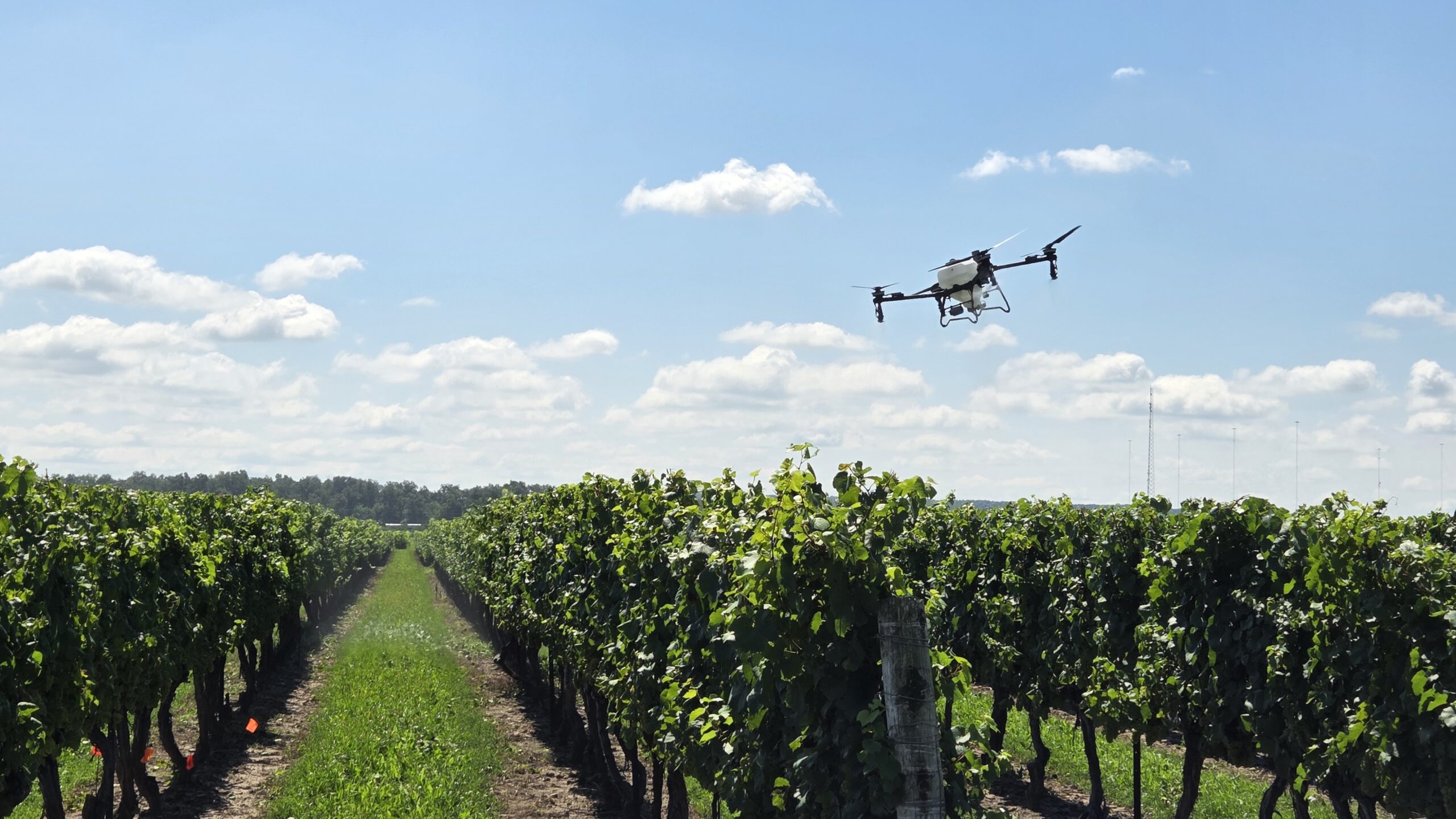
    Rotary atomizers, either from rotary cages or spinning disks, are capable of producing sprays whose droplet size ranges are more uniform than those from traditional hydraulic atomizers. This produces advantages ranging from improved drift management to better use of available carrier volume. Rotary atomizers are popular with aerial applicators and are found on the majority of spray drones.
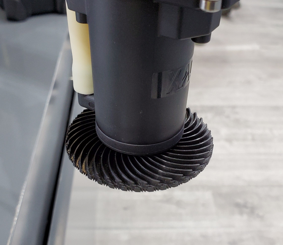
    Fig. 2: Rotary atomizer on a spray drone. Water is moved to the edge of a serrated disk by centrifugal force, forming ligaments that break into droplets

    Rotary atomizers create finer sprays when their rotational velocity is increased, or when the flow rate of the nozzle is decreased. In both cases, the ligaments formed at the periphery of the atomizer are thinner and will break up into smaller droplets. One disadvantage of rotary atomizers is the limited flow rate that they can atomize. For high flow rates, rotary cages, which break up the spray liquid by passing it through a series of wires mesh stages, are used. These require a fair amount of power, making them impractical for most smaller drone sprayers. 

    Droplet size ranges

    All hydraulic agricultural sprays are said to be polydisperse. This means that they are made up of a number of droplet sizes ranging from perhaps 5 µm to 1000 µm, or even 2000 µm or more for low-drift nozzles. How should the spray cloud be described?

    The vast majority of droplets in hydraulic sprays are small. In any sample of flat fan nozzles, low drift or not, about 80 to 90% of the total number of droplets will be less than 150 µm in diameter. This held more or less true for a wide range of nozzles. As a result, using a traditional weighted average droplet diameter was not useful as a descriptor because the abundant sizes would always control the outcome even though they contained a minority of the spray volume. The contribution of the larger, but less abundant droplets would be hidden with an arithmetic mean.

    Any other descriptors based on droplet number alone, such as mode (the most frequent size class) or median (the size class above and below which were an equal number of droplets) are equally dominated by the high abundance of the smaller droplets.

    To solve this problem, droplet diameters can be converted to their volume equivalent using the formula
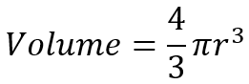

    Where r is the radius of the droplet.

    This is relevant because the dose of pesticide in a droplet is related to its volume. It’s important to understand the contribution of relatively few larger droplets in terms of how this dose was received by plants.
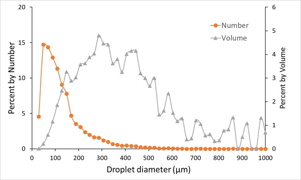
    Fig. 3: Number and volume distributions of a typical agricultural spray (Wilger SR11005 @40 psi)

    Thus we arrive at a volumetric distribution, where each diameter is described by the proportion of the total spray volume it represents. That volume represents the dose of spray. Now we have some practical meaning of the numbers.

    First we generate a cumulative volume distribution. The volume contained in each size fraction is expressed as a percentage of the total volume and these are added together.

    The cumulative distribution can now be divided into benchmark values so we can get values that differentiate various sprays. The key ones of interest are the 10th, 50th, and 90th percentile. The 10th percentile, known as the DV0.1, is defined as the diameter below which is 10% of the total volume of the spray. DV0.5 and DV0.9 likewise describe the diameters below which are 50% or 90% of the spray volume, and the former is more commonly known as the Volume Median Diameter (VMD). Recall that the median is the value that divides a distribution in half by number, therefore the 50th percentile is also the median.
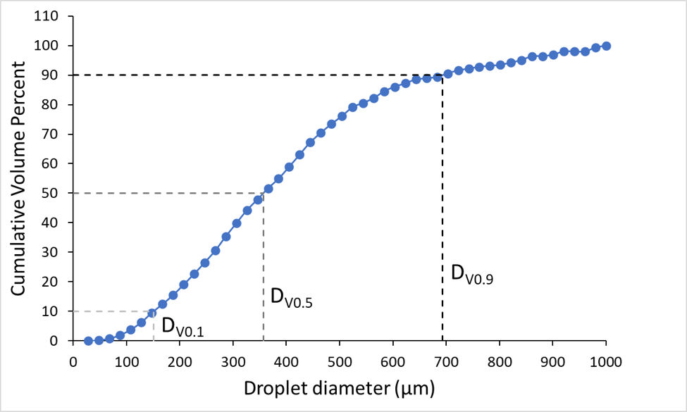
    Fig. 4: Cumulative volume distribution of Wilger SR11005 @ 40 psi. Dashed lines show DV0.1, DV0.5, and DV0.9.

    The VMD is the benchmark value, it can be thought of as the diameter near which the majority of the dose is delivered. The DV0.1 can serve as a drift index, describing the diameter that contains the smaller droplets. Sprays that are more drift-prone have lower DV0.1 values. The DV0.9 can be an index of the droplets that may not be able to contribute much to product efficacy because they are too big to cover much area, and they are likely to be very rare, possibly missing the target altogether. Higher DV0.9 values indicate that more of the spray may be lost to large droplets that will likely rebound.

    All of these parameters are related to each other. A finer spray will have lower DV0.1, DV0.5, and DV0.9 values. But it is not necessarily correct to say that a spray with a lower DV0.5 will have less drift potential. Some nozzles, by virtue of their design, can have smaller driftable size fractions as well as a lower DV0.5.

    One of the main reasons that sprays of equal DV0.5 may have different behaviours in the environment is their Span. Relative Span describes the uniformity of the droplet sizes in a spray. A perfectly uniform spray (containing droplets that are all the same size) will have a span of 0 because all three volumetric parameters will be equal.

    We sometimes encounter the Sauter mean of a spray, which can be defined as the diameter of a drop having the same volume/surface area ratio as the entire spray. This is useful when surface area is of importance, such as in combustion or evaporation.

    The popularity of laser measurement systems, and their ability to measure droplets that previously escaped detection, was a boon to the spray industry. But it quickly became clear that simply comparing these parameters was problematic. Each laser system, and indeed each laboratory that used them, seemed to create their own unique values for the same nozzles. We will explore the solution to this problem in Part 3.
  • What is Spray Quality, Part 1 – Measuring Droplet Size

    What is Spray Quality, Part 1 – Measuring Droplet Size

    It’s often been said that droplet size is the most important factor governing spray operation success. Both spray drift and pesticide efficacy depend to a large degree on droplet size. For something this important, the droplet size information from nozzles ought to be accessible and easy to understand. 

    There are a few problems to overcome before we get there.

    The first is the difficulty in measuring droplets in the first place. Spray droplets are very small and evaporate quickly.  In the early days of spray technology research, sprays would be captured on a surface and individual droplets measured and counted under a microscope. A common approach was to use magnesium-oxide coated glass slides. The magnesium oxide layer was soft, and an impinging droplet left a tell-tale crater behind, much like those found on the moon’s surface. This allowed the analysis to be done after evaporation. Magnesium oxide does a great job but relies on droplets having enough momentum to leave their mark. There is also a spread factor (ratio of crater diameter to droplet diameter) that has to be known.

    Water-sensitive paper (WSP) is the modern version of this concept, and we’ve written much about the topic. Jason in particular has done a deep dive on how WSP works and how it’s analyzed.

    We can also add dye to spray mixtures to see deposits on various glossy paper surfaces.  The resolution of the dye-droplets can be better than those from WSP but their deposits can also be so faint that they pose thresholding and analysis problems.

    The great thing about impingement methods like WSP is that they’re easy to use, and they are particularly useful for a quick visual and qualitative assessment of coverage. If wanted, coverage can be quantified by scanning the WSP for percent area covered or deposit density.

    Droplet size determination is problematic on WSP because one needs to know the spread factor (how much larger the deposit is compared to the in-flight droplet that caused it) to back-calculate the original size of the in-flight droplet.

    Spread factor depends on droplet size, velocity, formulation, and the nature and orientation of the surface it’s collected on. The SF formula provided by the paper manufacturers is a good start but it is far from perfect.

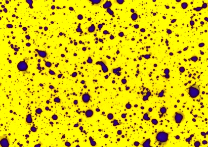
    Fig. 1: Water-sensitive paper (WSP) treated with a Very Coarse spray at about 100 L/ha. Note the coalescence and overlap of some deposits.

    In addition, the overall droplet density has to be low enough to avoid overlaps or coalescence. Usually a water volume over 50 to 100 L/ha will create issues. The WSP also has to collect the droplet in the first place. Smaller droplets often move around larger objects such as a leaf, or a similar sized piece of paper. If they impact at a sharp angle, the deposit will be elongated due to smearing and that creates additional difficulties.

    Even if the paper collected the smallest droplets, they may not appear as stains. Droplets below a certain diameter (about 50 µm) do not leave a visible deposit on the paper. 

    So, while WSP is a great tool for visualizing a deposit, its limitations usually prevent it from being used to accurately measure the droplet size spectrum of a spray. 

    The Rise of the Laser

    In the 1970s and 80s, we saw the introduction of laser-based droplet size measurements. With these, a spray simply needed to be directed into a such an instrument, and it very quickly determined the diameter, and in some cases, the velocity, of the droplets. The principles employed by various laser instruments differed, and although one could now rapidly obtain data in-situ, the numbers among the instruments didn’t always agree.

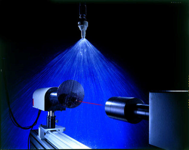
    Fig 2: Laser instruments help to measure droplet size of sprays (photo source: TeeJet)

    The Most Common Laser Systems

    Laser diffraction: One of the first droplet sizing instruments is manufactured by Malvern (https://www.malvernpanalytical.com/en), and is still in use today. A laser beam passes through a spray cloud. The system uses a laser diffraction principle that works as follows, according to Malvern: “Large particles scatter light at small angles relative to the laser beam and small particles scatter light at large angles. The angular scattering intensity data is then analyzed to calculate the size of the particles responsible for creating the scattering pattern, using the Mie theory of light scattering.”

    To calculate the droplet sizes responsible for the scattering behaviour, the laser system has light-sensitive sensors in concentric circles behind the spray plume. When a sensor in the middle of these rings picked up a signal, it likely originated from a larger droplet because of its lower light scattering properties. Sensors further from the centre picked up smaller droplets. The system thus had an idea of the relative frequency of the various droplet sizes in the spray cloud and modelled these according to the classic Rossin-Rammler spray distribution model, from which descriptive parameters are calculated.

    Laser diffraction is the most popular method for in-situ droplet sizing. The company Sympatec (https://www.sympatec.com/en/) also offers a system that competes with Malvern that is found in many labs.

    Laser Shadowing: The Particle Measuring Systems (PMS) system was one of the earliest laser systems. It was a very compact and sturdy system that shone a laser light at the spray cloud and the droplets in that cloud cast shadows against a sensor array a fixed distance away. The size of these shadows could then be measured to arrive at a droplet size distribution. The PMS was particularly good at measuring small droplets.

    Although long discontinued, the PMS system had the basic appearance of a torpedo and was often mounted on aircraft or in wind tunnels to measure cloud aerosol sizes. Very cool. The company still manufactures other particle measuring devices (https://www.pmeasuring.com/).

    Pulsed Laser Illumination: This is a different approach to the laser shadowing of the PMS system. Oxford Lasers systems (https://oxfordlasers.com/) use a video camera to view the spray cloud and freeze images from using a very high frequency pulsed laser light. This light illuminates the cloud briefly which allows a still image to be briefly displayed.  Image analysis then measures the diameter of each particle in the image, adjusting for out-of-focus images.  It’s possible to analyze the speed and direction of the particles by comparing the particle position in subsequent images. This system is quite popular among scientists due to its ease of use. A portable unit that can be deployed in fields is available.

    Phase Doppler: In the mid 1980s, a system was developed that uses the Doppler principle to measure both the speed and diameter of droplets. Two out-of-phase laser beams intersected in a spray cloud, and a droplet passing through the intersection point created a Doppler burst that signalled the speed of the droplet. The burst signal also contained information on the droplet diameter, derived from a frequency shift of the two laser beams utilized in the system. This system has very high data acquisition and was the first to create a temporal sample of the spray, increasing the accuracy of the droplet size measurements.

    Initially brought to market by Aerometrics (later acquired by TSI) and called the Phase/Doppler Particle Analyzer (PDPA), it is now mainly offered by Dantech systems (https://www.dantecdynamics.com/).

    Sampling Bias: Temporal vs Spatial

    It’s not straightforward to measure a sample of moving objects. It may seem intuitive that if one wants to know how many objects are present, taking a picture and counting the objects would provide the answer. But when objects move at different speeds, that answer will be incorrect because the slower moving objects will be over-represented.

    Let’s assume you’re working on a traffic count project to understand the number of people crossing a bridge either walking or cycling. Let’s also assume that one walker and cyclist depart for the bridge every 5 seconds, i.e., there are the same number of each. If you wait until the bridge is full of people crossing and take a picture it will show more people walking on the bridge than riding bicycles. That is because the bicycles are faster and many will already have left the frame.  Thus counting the number of people in the picture over-estimates the number of walkers because they move slower.

    The same problem arises with these laser systems because in a hydraulic spray, the smaller droplets move slower than the larger droplets. Any system that takes a picture and counts what’s in it will have what’s called a spatial sample, overestimating the slower (smaller) droplets.

    A temporal sample can measure the velocity of the droplets and therefore account for their speed, giving a more accurate measure of the abundance of the droplets. In the case of the PDPA, it acheives this simply by counting all the individual droplets that pass, in sequence, through its meassurement area, called the probe volume. As they pass, it notes their velocity and diameter.

    To address this issue with a spatial sampling instrument, many labs now use wind tunnels and direct the spray to be tested with the wind direction. This forces the droplets to move at more or less the same velocity as the wind, eliminating or at least minimizing the speed differences before the droplets reach the laser instrument.

    WSP produces a temporal sample because it ultimately catches all droplets, but it has different types of sampling bias. Large deposits usually cover smaller ones. Smaller droplets may not impact on the target due to poor collection efficiency. Small droplets may dry too quickly to leave a visible stain. As a result, even if we had accurate spread factors, we would tend to under-estimate the number of smaller droplets, opposite of the error of spatial systems.

    Scanning the pattern

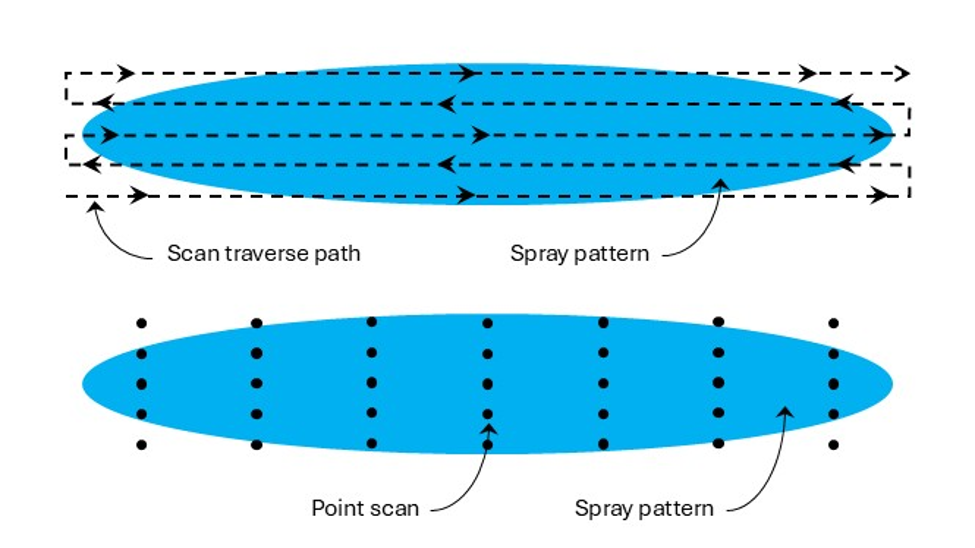
    Droplets are not distributed uniformly within a spray pattern. In a flat fan nozzle, for example, the centre of the pattern contains the smaller droplets. The outside edges of the pattern contain fewer small droplets and more large droplets. Some laser systems have a very shallow depth of field, and the PDPA is a point-measurement. As a result, it is not accurate to simply point the measuring device at a single location of the spray pattern. Accurate droplet size spectra from lasers requires a thorough traversing scan of the spray pattern along at least its long axis, and preferably two or more such traverses at increasing distances from this central axis. The scanning method would likely need to be adjusted to suit various types of atomizers, such as hollow cone nozzles.

    If no traversing mechanism is available, it is acceptable to measure the spray at several discrete locations and then merge the data prior to analysis. In all cases, three replicate samples should be taken so that an estimate of variability is available.

    Many labs, having compared a full scan with many traverses to those with fewer traverses have opted for a simple back and forth traverse with little loss in accuracy.

    Fig. 3: Possible ways of scanning a spray pattern for droplet size analysis. Top: traversing scan. Bottom: point scan

    Sometimes sprays are atomized within a chamber to prevent the droplets from contaminating the surrounding area if they contain any active ingredients. These chambers can also add measurement errors from, say, small droplets that recirculate within the chamber, or due to any glass surfaces through which the laser lights must pass. These all need to be considered, as they add to the many variables that create different results even when comparing identical sprays between labs.

    The next topic, covered here, is how to use the information we gather from droplet measurements. As you might expect, this is also not as straightforward as it seems.

  • Sprayer Productivity for Smaller Scales

    Sprayer Productivity for Smaller Scales

    Travel is an amazing teacher. It exposes assumptions and replaces them with real life experiences.

    On a recent trip to New Zealand, I learned a valuable lesson in sprayer productivity. I had long talked about wider booms being a key factor, being an easy change that allowed more area to be covered per pass. I had assumed large fields, large tanks, and fast fills as part of that system, and validated it with calculations and observations.

    During that trip, I learned that things look really different when the landscape dictates certain limitations. In places like New Zealand, fields tend to be smaller, as expected, with the longest run averaging 300 m or so. Sprayers are also smaller capacity, with trailed sprayers typically fitted with a 24 m boom and a 3000 L tank. Mounted sprayers, commonplace on the North Island, may have smaller tanks and booms, with 2000 L and 18 m width a reasonable average. Self propelled sprayers are not common on farms, but custom applicators use them.

    Tender systems (called bowsers) are also rare. Most applicators return to the farm yard, or another nearby water source, to fill. A single filled sprayer can often do that entire field, so moving to a new field and re-filling are part of the same workflow.

    Some very interesting things happened when such a scenario was analyzed.

    We used a newly re-vamped Productivity Calculator (below) to make the calculations.

    Some basic configurations were assumed. All sprayers travelled 15 km/h when spraying, and turned in one headland at 8 km/h. The tank remainder that necessitated a re-fill was set at 5% of tank volume. Tank cleaning was assumed to be required every four tanks, taking 60 minutes. Sprayers were typically refilled in the farm yard or a nearby water source, requiring a ferry (transport) time of 15 minutes each way.

    The first scenario was the base configuration, from which one factor was changed in each iteration to examine the magnitude of the change. With the 24 m boom, 3000 L tank, 200 L/ha application volume, a field length of 300 m, a loading time of 30 minutes, and a loading location that required a 30 minute round trip, net productivity was 8.0 ha/h. 22% of engine hours were spent spraying, the remainder was lost to turning at the end of a run, driving to the loading location, loading the sprayer, and cleaning it. We will call that the spraying efficiency.

    Because wider booms are successful in improving productivity in western Canada, we examined the practice for smaller farms. Increasing the boom width from an average 24 m to 36 m yielded the first surprise. Productivity only increased to 8.5 ha/h (7%), and spraying efficiency was reduced to 16%.  The problem appeared to be that the wider boom dispensed with the tank contents faster, requiring more frequent filling. And that of course was the big time user, accounting for 60% of the engine hours. 

    The next step was to examine a larger tank (5000 L), keeping the original 24 m boom. This change yielded big results, with productivity jumping to 11.1 ha/h, a 33% increase from the base condition. The larger tank reduced the frequency of filling, and that reduced its drag. Spraying efficiency jumped to 31%.

    Another way to achieve a lower filling frequency is to lower the amount of water applied. This is a bit risky, as water volume is likely to most important variable that ensures good spray success, especially when dealing with dense, high yielding crop canopies. In cases where canopy penetration isn’t an issue, and systemic products can be used, less water may be an option. A modest decrease from 200 to 150 L/ha was tested.

    Again, a large jump in productivity was observed, from the base of 8.0 ha/h to 9.7 ha/h, about 21%, resulting in 27% spraying efficiency.

    What if fields were merged, or shelterbelts removed, resulting in longer spray passes? These would reduce the time lost to turning, which had been 8% of engine hours for the 300 m pass.  We decided to test a 600 m pass. But while it reduced the proportion of time spent turning to 4%, overall productivity barely nudged to 8.3 ha/h.  That’s a 4% improvement, not worth removing any trees over.

    One of the biggest game-changers in sprayer productivity has been the 3” transfer pump and efficient product induction systems. Reducing fill time from 30 to 15 minutes did have a large effect here too, increasing productivity to 9.3 ha/h, a 16% increase from the base. There remain inefficiencies in the system, such as the time spent with partial jugs that require measuring. A faster pump doesn’t address these. But perhaps a closed transfer system can.

    With the travel time associated with a home fill being such a large time consumer, introducing a field-based tendering system was expected to have a large impact. We combined this with a fast fill because a proper tender unit would have the larger pump. And the results were impressive, a jump to 13.7 ha/h. That’s a 72% increase from the base scenarios, boosting spray efficiency to 38%. 

    The final scenario involves two large changes. A new, larger sprayer with a 5000 L tank and 36 m boom, combined with a fast fill tendering system. And the results were equally large, boosting productivity to 19.8 ha/h, more than doubling the performance of the base condition (a 148% improvement). Spraying efficiency did not increase further from the fast-filling tendering system alone, because the faster filling was accompanied by the faster emptying of the wider boom.

    What is the value of this study? For one thing, we learned that a change that works in one geographic area may not work in another. For these smaller field scenarios, the benefit of a wider boom was undermined by the long downtime during fills. And obtaining a tender system when a single sprayer fill can cover a whole field wasn’t a slam dunk like it is elsewhere, where a field often requires several fills.

    Does a producer actually need to spray everything faster? The answer will depend on each farm. A general observation we’ve made is that the windows of opportunity for spraying are getting narrower. Restrictions on wind speed or temperature leave fewer hours in a day to get the spraying done. The risk of falling behind is lurking. And that means that application may not get done when they’re most effective. Disease may have progressed. Weeds will have grown. Crop safety may be challenged. Being even a little more productive can help mitigate all those risks.

    If nothing else, it’s critical for an applicator to know where the time goes. Use the calculator. Only then can you be strategic about correcting a problem. 

  • Improve your Drone Spraying Productivity

    Improve your Drone Spraying Productivity

    Drone operational settings such as capacity, speed, and swath width are useful figures for calculating productivity, but they only describe the airborne portion of the job. A commercial application business must also transport water, mix product, charge batteries, and establish an efficient staging area that is both safe for operators and maintains drone connectivity. If any of these functions fall behind, productivity suffers.

    We used one Ontario operator’s experience to show why drone productivity is measured as a complete application system, and not just flight settings. Download our offline version of the calculator or try it online at the end of this article. It has been pre-populated with the metrics from a corn fungicide case study. Agronomic context matters when considering operational settings.

    How to use

    Adjust a single variable to see what effect it has on productivity. Return the variable to its original value, then change another. That way you can explore the relative influence of each variable on the overall job. This calculator is a work in progress, so expect changes each time you come back to it.

    Which factors matter most?

    The factors that have the biggest impact on productivity are situation-specific, but here are some generic observations:

    • While swath width and flight speed play a role, both are limited by the agronomic realities of the job, so there may not be much latitude to change these figures.
    • Water volume used has an impact on productivity, but once again there are agronomic considerations. Too low a volume can compromise product efficacy and contribute to off target drift, and quite often the minimum volume is stipulated on the product label.
    • The drone’s tank capacity depends on the model, but maxing it out may not be the best option. Some large drones suffer reduced battery life and slower acceleration when filled completely.
    • The ferrying distance between where the drone empties and the staging area is variable throughout the job. This is why the calculator asks for an estimated average. Minimizing this number is an important consideration, but it may not be subject to change because the staging area location is primarily a function of field access, drone connectivity and operator safety.
    • The time to fill the drone and swap batteries plays a large role in productivity, depending on how many cycles (aka sorties) are involved. Small improvements here compound into big impacts.
    • Tender water tank capacity (and refills) play a big role as well. If the operator has to stop spraying to retrieve more water, the drone isn’t spraying.

    Enter the parameters from your own operation to see what happens. The drone settings get a lot of the attention, but it’s tendering efficiency that keeps it earning.

    Drone Productivity Calculator

    Estimate field productivity, application time and water-support requirements with live operational modelling.

    Step 1

    Field and flight inputs

    seconds
    passes
    Step 2

    Water and support logistics

    minutes
    min/stop
    Do water retrievals halt operations?
    Yes
    Step 3

    Advanced flight model

    %
    %
    Live productivity estimate
    0.0
    Total operation
    Spraying share
    Productivity time
    Water required
    Water tripsadditional retrievals

    Time by activity

    total minutes

    Operational balance

    Operation details
    Ready to share this scenario?

    Download a branded, print-ready report of the current results.

  • Assessing wheat head coverage from Defy 3D and 3D Ninety nozzles

    Assessing wheat head coverage from Defy 3D and 3D Ninety nozzles

    We’ve been here before, haven’t we? I could rehash the explanation of why wheat head coverage is important, and define the variables involved, but perhaps you’re already in-the-know. Instead, new readers (and those requiring a refresh) can go give this article and this article a quick read and then come back. I’ll wait.

    Why perform another wheat head nozzle assessment? Primarily we do it so you don’t have to, but in this case there’s a specific problem we’re trying to solve and a “new” nozzle to explore.

    The problem (and some history)

    Let’s digress a little and use the historical experience shared by Clean Field Services (CFS) in Drayton, Ontario (cooperators in this study), to explain the problem and our objective.

    As broadacre sprayers evolve, nozzle technology has been lagging. Consider a basic field sprayer equipped with a centrifugal pump. Its performance curve exhibits a direct relationship between flow rate and pressure. In this case, the operator relies on a rate controller to bypass flow to maintain a target application rate across a range of travel speeds.

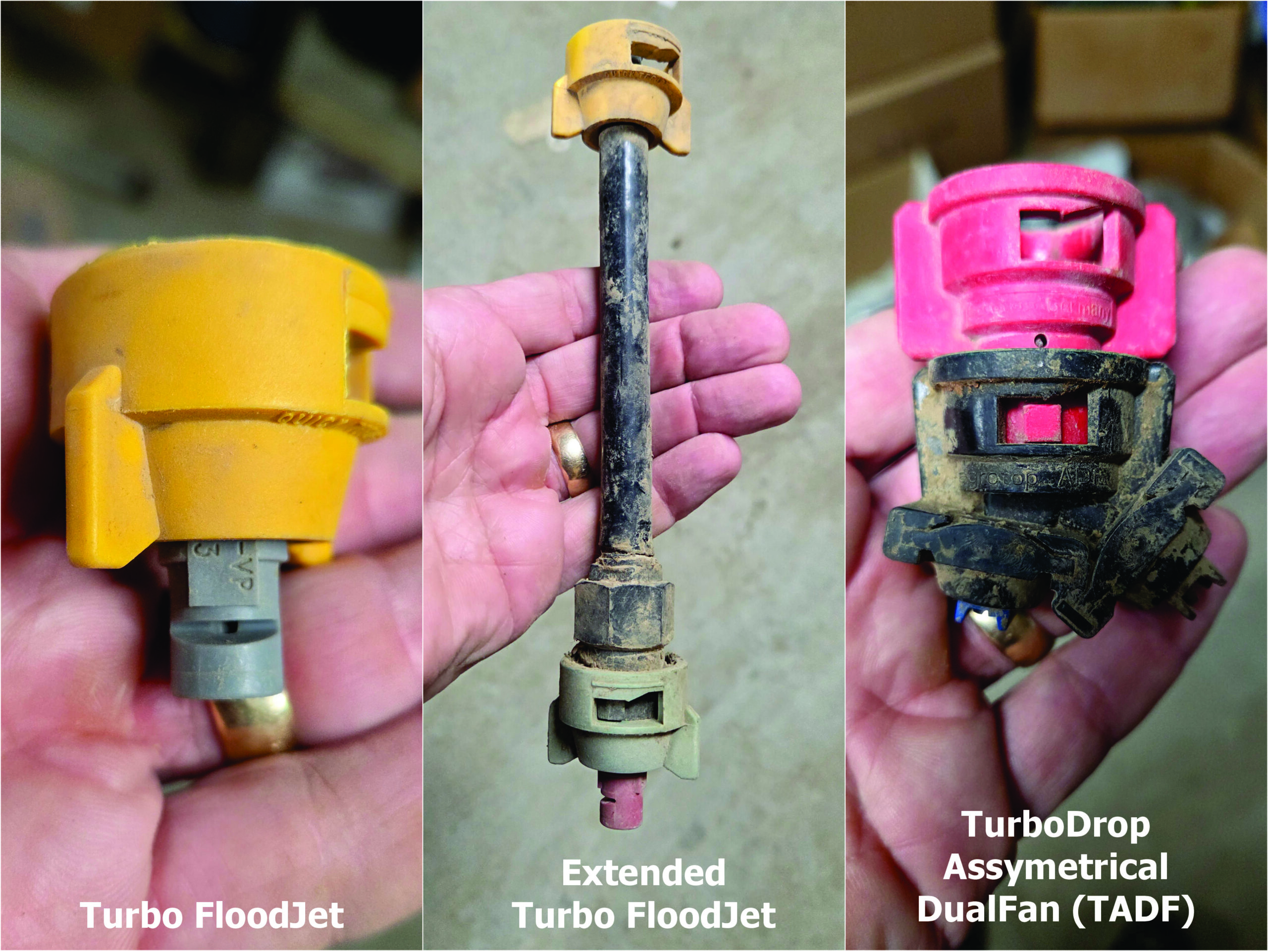
    However, bypassing changes system pressure, which inadvertently changes the average droplet size. Basically, increasing travel speed reduces droplet size and vice versa. This was the manner of sprayer used in Ontario more than 20 years ago when researchers demonstrated that TeeJet Turbo FloodJets, alternated front-to-back, provided excellent coverage of wheat heads at the T3 timing. This is what Clean Field Services used.

    However, some booms have obstructions that interfere with the aggressive spray angles produced by wide-pattern nozzles such as the Turbo FloodJet. CFS experienced this when they got a RoGator in 2012 and later an R-series Deere in 2017. At one point they tried using extensions to clear the obstruction, but this proved to be a nuisance and interfered with folding. They settled on GreenLeaf Technologies’ TurboDrop Asymmetric DualFan (TADF), which worked great, until the sprayer changed again.

    A visual history of wheat nozzles at Clean Field Services.

    Pulse Width Modulation

    Sprayer plumbing and control systems have evolved. The introduction of pulse width modulation (PWM) technology changed the way rate control is achieved. Rather than regulating flow by altering pressure, PWM intermittently interrupts flow at the nozzle. This decouples flow rate from pressure, preserving droplet size across a range of travel speeds. Most air induction (AI) nozzles, such as the TADF are not approved for use with PWM systems.

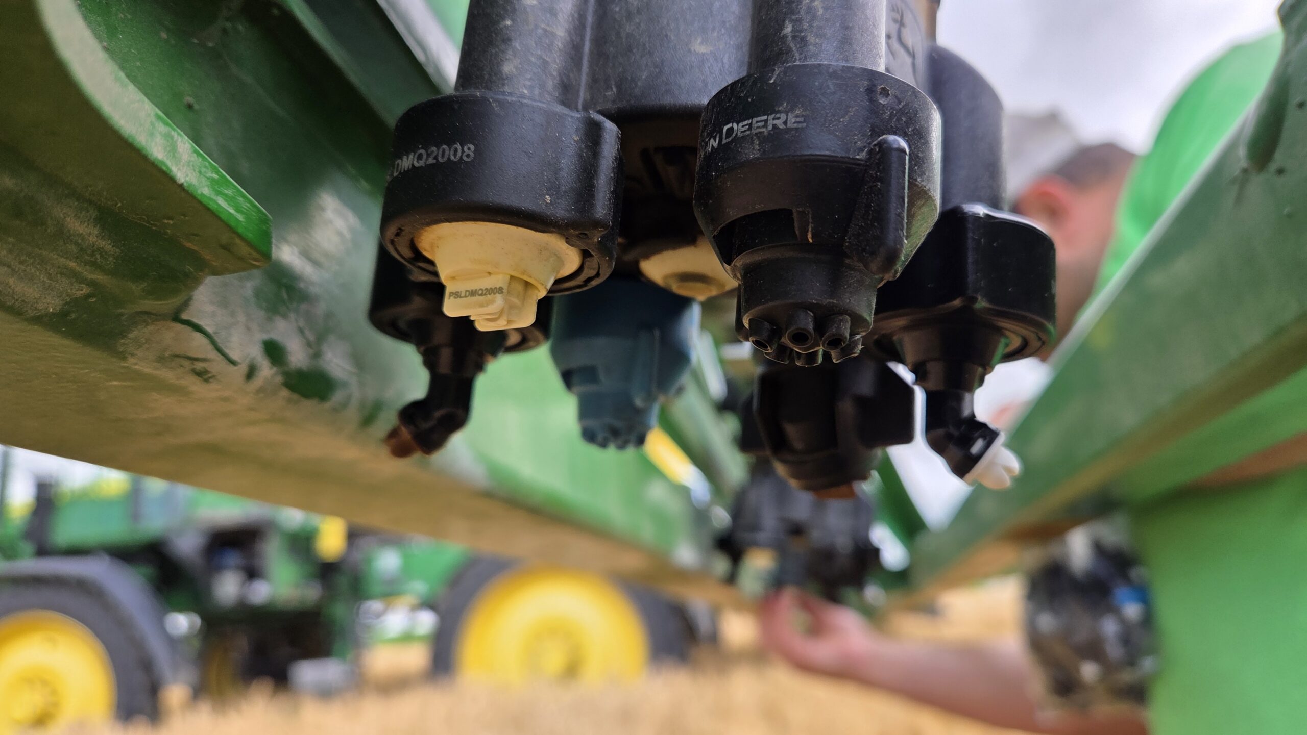
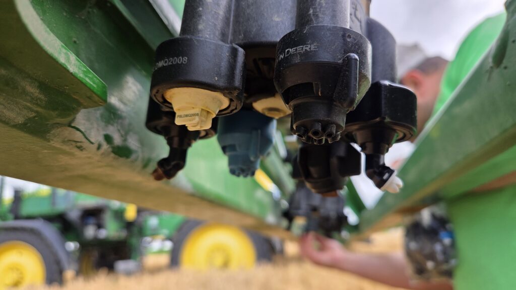
    John Deere’s ExactApply PWM system became available in 2017, and CFS got one in 2018. Operators could mount two nozzles in each position, creating opportunities for interesting new configurations. One of the recommended nozzles was the Defy 3D, which features a 38° angle and was developed by Hypro in collaboration with Syngenta to help control blackgrass in the UK. It performed well in drift-reduction studies relative to conventional flat-fan nozzles.

    Welcome to Canada

    CFS mounted a single Defy 3D ’08 in each nozzle body, and had problems. Canadian sprayer operators, on average, drive faster than their UK cousins. Even with PWM, the largest Defy 3D tip (the ’08) required a flow rate that increased system pressure, which in turn led to a drifty experience. Bad in itself, but also not ideal for angled applications, because finer spray deposits with the wind rather than ballistically.

    They tried throttling back, slowing down and/or adjusting water volumes, but felt they never really dialed it in. They settled on a Defy 3D ’08 in the B (rear) position, and an ’05 in the A (front) position at 21 km/h (13 mph) to apply 156 L/ha (16.67 gpa).

    Exploring a solution

    Wouldn’t it be nice to have your cake and eat it too? Drive faster, apply higher volumes and still mitigate drift? Enter the 3D Ninety, with claims of good fungicide utility while producing a significantly coarser droplet than the Defy. They came out in 2021, and yet they are still difficult to find in North America. This study establishes baseline panoramic coverage from the Defy 3D, then benchmarks it against the 3D Ninety and a hybrid configuration at a faster travel speed.

    Experimental design

    The trial took place in a mature wheat field in Drayton, Ontario on July 22, 2026. Temperature was 15°C, and while generally windy, we operated in an area protected by a windbreak, reducing windspeed from an ambient 18 km/h to an average 8 km/h at boom height.

    Sprayer settings

    A John Deere See and Spray Premium (410R) was used in the study. For each condition, we isolated a section of seven nozzles in the middle of the left and right booms (as far as possible from boom tip and chassis). Nozzles were on 50 cm (20″) spacing, so this spanned 2.7 m. The sprayer was set to a 70% D.C., and the boom was 50 cm (20″) above the wheat heads. The treatment conditions were as follows:

    TreatmentForward NozzleRear NozzlePressure (psi)Travel speed (mph)
    1’05 Defy 3D’08 Defy 3D2513
    2’05 3D Ninety’08 3D Ninety4016
    3’05 Defy 3D’08 3D Ninety4016
    Operational settings and nozzles for each treatment.
    In all treatments the ’05 faced forward and the ’08 faced back.

    Samplers

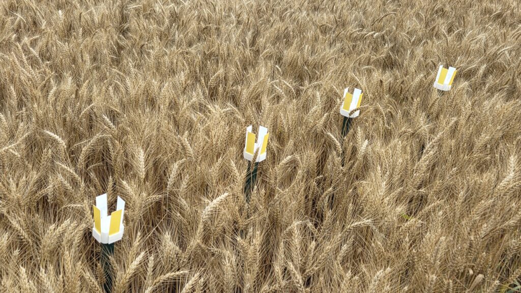
    A series of four posts were positioned in the wheat, spaced 0.5 m apart and centred on the corresponding section of nozzles. The samplers were SpotOn water sensitive papers (WSP) mounted in custom holders to orient four papers at 90° to the sprayer: Advance (facing the sprayer), Left, Retreat (facing away from the sprayer) and Right.

    A series of samplers positioned at wheat head height, 50 cm apart, centred on the swath produced by the section of seven trial nozzles.

    A parallel tramline approximately 1 m from the samplers provided access. The sprayer began spraying 15 m (50 feet) before the samplers and continued spraying the same distance beyond them. Once the spray settled, the samplers were retrieved. A single pass represented a repetition and there were three passes per treatment.

    Papers were digitized using a DropScope (SprayX) and the analysis was performed in R (v. 4.6.0), leveraging the rpy2 library for integration with Python within the Colab environment.

    What we saw

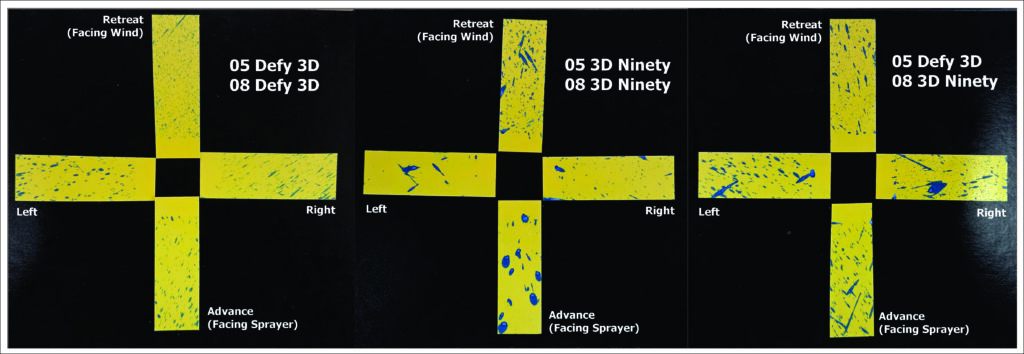
    The following image shows a typical coverage pattern for each treatment. While WSP is not able to determine droplet size accurately, it can certainly reveal relative differences. It was clear that the Defy 3D produced smaller droplets than the 3D Ninety, and that there were far more of them. The hybrid condition shows a more heterogeneous coverage pattern, which would be expected given it represents a greater span of droplet sizes than either nozzle design used alone.

    Typical coverage pattern from each treament.

    Defy 3D

    3D Ninety

    Hybrid Defy 3D and 3D Ninety

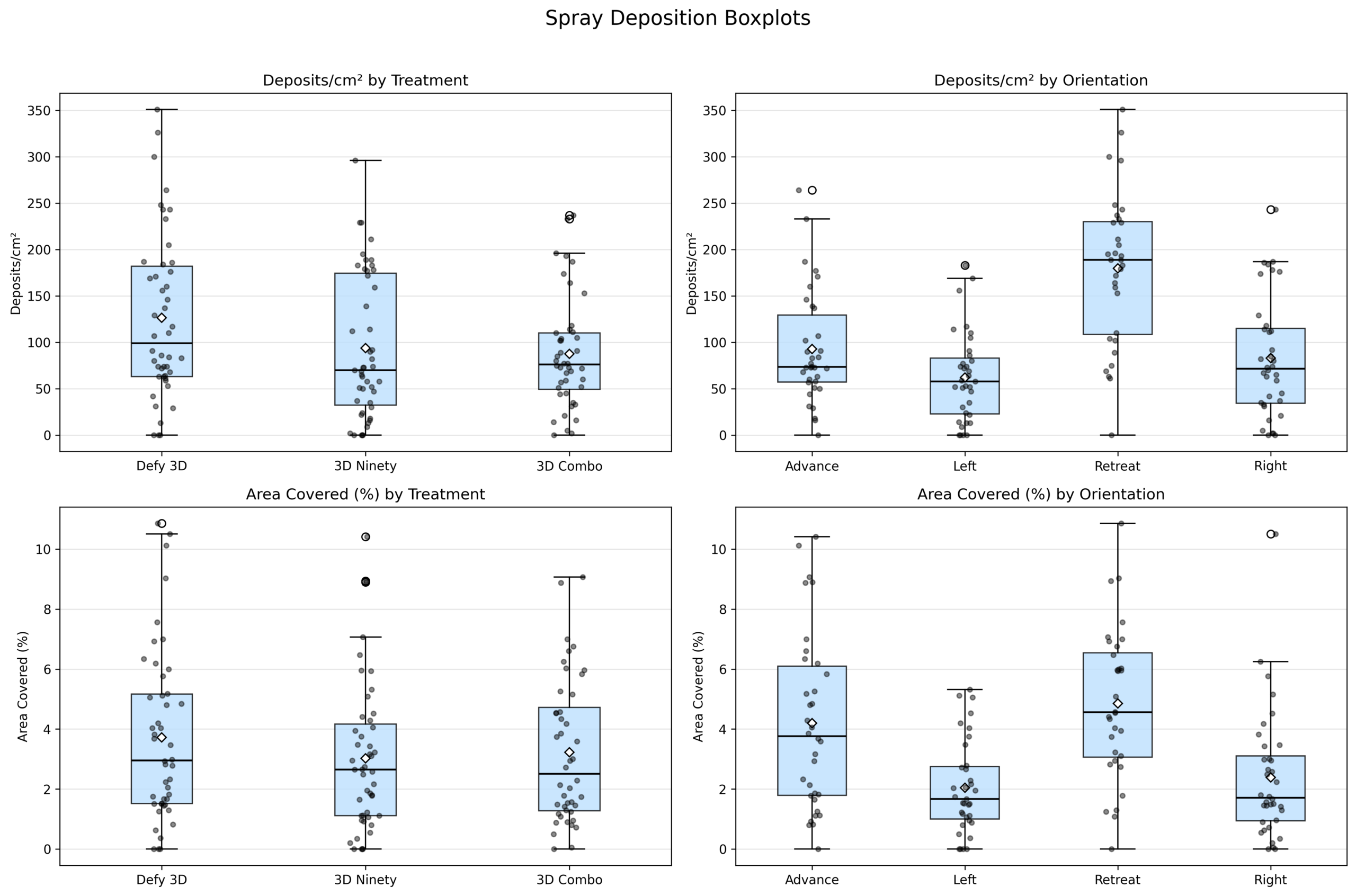
    Continuing with general observations, we can average the coverage measured on each plane, on each sampler, for each treatment. When spoiled samplers were removed from the study (it happens), coverage can be described as either the area covered, or the number of deposits per area. With no exploration of variability, we see that the Defy 3D resulted in the greatest average coverage as represented by either metric.

    TreatmentnMean Area Covered (%)Mean Deposits/cm²
    Defy 3D463.73126.35
    3D Combo443.2287.64
    3D Ninety473.0293.77

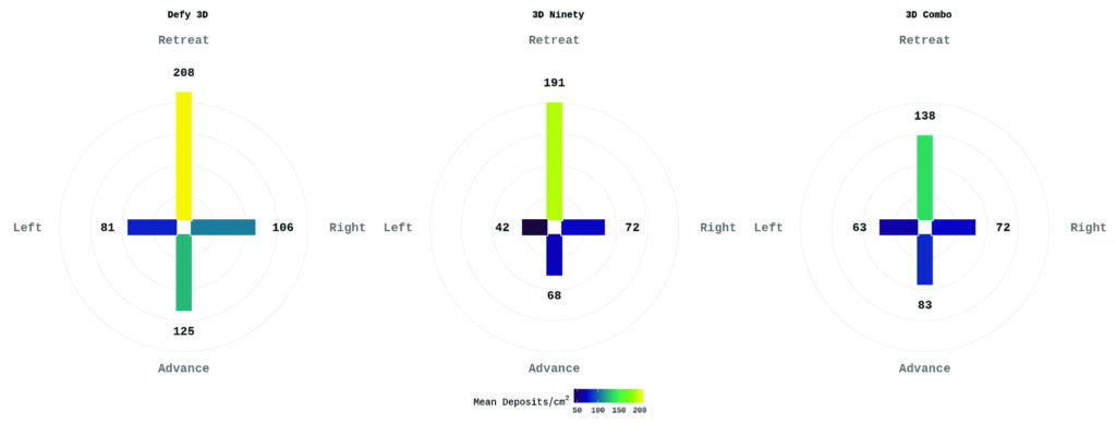
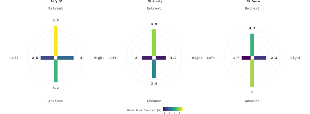
    We can drill down and explore coverage by WSP orientation as well, this time including some measure of variability (standard deviation). As a matter of housekeeping, there was no evidence that repetition or post position had any meaningful bearing on coverage results (Pearson p of 0.422 and 0.455 and Spearman p of 0.267 and 0.217). We see the highest average number of deposits on the retreat side (facing the wind) in all treatments. Similarly, and excepting the combination treatment, we see the greatest average area covered on the same plane.

    TreatmentOrientationnMean Deposits/cm²SDMean Area Covered (%)SD
    3D ComboAdvance1183.0053.584.982.80
    3D ComboLeft1163.3638.071.671.24
    3D ComboRetreat10138.2058.384.121.93
    3D ComboRight1272.0063.842.291.93
    3D NinetyAdvance1167.8252.923.413.38
    3D NinetyLeft1242.2549.831.961.61
    3D NinetyRetreat12191.1754.204.892.07
    3D NinetyRight1271.6750.301.871.46
    Defy 3DAdvance12124.9265.484.192.64
    Defy 3DLeft1280.7549.752.481.74
    Defy 3DRetreat10207.70115.845.553.45
    Defy 3DRight12105.5875.922.982.83

    We can illustrate this using box and whisker plots, which show all the data as well as the relative span of each treatment. This makes it easier to compare the treatments and determine if any differences in average coverage were significant or not.

    We can illustrate coverage in an even more intuitive manner using a rosette-style graph. Here we see the average deposit density or the percent area covered for each treatment on each plane. Note that the discrepancy between the Advance (shadowed by wind) and Retreat (wind-facing) side is far greater when the coverage is represented by droplet counts rather than area covered.

    Average coverage on each plane for each treatment, as represented by deposit density.
    Average coverage on each plane for each treatment, as represented by percent area.

    Interpretation and discussion

    Deposits/cm² and percent area covered were strongly positively associated (r = 0.75), indicating that higher deposit counts generally corresponded to greater percent coverage. The relationship wasn’t perfect, suggesting that other factors also influenced coverage and leaving room for interpretation.

    The Defy 3D produced the highest overall coverage, as reflected in total deposit counts. This is consistent with the fact that it emits a higher proportion of finer droplets relative to the 3D Ninety. While finer droplets can improve coverage, they are also more prone to drift and tend to deposit on the downwind face of vertical targets. We have evidence of this in all treatments, which showed more deposits on the Retreat (windward) face than on the Advance face, which was sheltered from the wind.

    This deposition pattern is likely influenced by the rear-facing nozzle configuration (an ‘08), which delivers a higher application rate than the forward-facing nozzle (an ‘05). With higher boom heights or stronger wind conditions, this configuration may be less effective, as reported in previous studies. In this comparison, the Defy 3D also exhibited the greatest variability, suggesting greater sensitivity to such conditions.

    The 3D Ninety and hybrid treatments were difficult to separate based on overall coverage. There was no significant difference in the magnitude of coverage between them, although the hybrid condition showed a more balanced distribution of deposits between the Advance and Retreat faces. In contrast, the 3D Ninety would be expected to produce a coarser spray that is less susceptible to deflection, assuming boom height is sufficiently low to maintain droplet trajectory. Despite this, it recorded more deposits on the Retreat face than the hybrid condition. We have no explanation.

    The hybrid configuration was designed to improve deposition balance by combining complementary spray characteristics. The forward-facing nozzle produced finer droplets, which can be carried along by the sprayer’s forward momentum to enhance forward deposition. The rear-facing nozzle produced coarser droplets at a higher application rate, compensating for lower droplet numbers while counteracting forward momentum to improve retreat-side coverage.

    Although the hybrid treatment appeared to provide a more even distribution of deposits between the Advance and Retreat faces, it is uncertain whether this would translate into improved biological efficacy. Further trials would be needed to evaluate whether this deposition balance leads to measurable yield gains.

    It is also important to note that both the 3D Ninety and hybrid treatments were applied at 25.7 km/h (16 mph), nearly 20% faster than the Defy 3D treatments. This indicates potential for higher productivity. Given the relatively balanced deposition observed, a combination of a forward-facing Defy 3D nozzle and a rear 3D Ninety nozzle may offer improved resilience to changes in boom height and wind speed while maintaining adequate coverage at higher travel speeds.

    Thanks to Clean Field Services for their participation in this study, thanks to Agflow Canada (Hypro / Shurflo) for donating the 3D Ninety’s, and thanks to Cesar Cappa, OMAFA weed specialist in horticulture for patiently explaining how to use R more effectively.