Category: Spray Basics

What is Spray Quality, Part 1 – Measuring Droplet Size
It’s often been said that droplet size is the most important factor governing spray operation success. Both spray drift and pesticide efficacy depend to a large degree on droplet size. For something this important, the droplet size information from nozzles ought to be accessible and easy to understand.
There are a few problems to overcome before we get there.
The first is the difficulty in measuring droplets in the first place. Spray droplets are very small and evaporate quickly. In the early days of spray technology research, sprays would be captured on a surface and individual droplets measured and counted under a microscope. A common approach was to use magnesium-oxide coated glass slides. The magnesium oxide layer was soft, and an impinging droplet left a tell-tale crater behind, much like those found on the moon’s surface. This allowed the analysis to be done after evaporation. Magnesium oxide does a great job but relies on droplets having enough momentum to leave their mark. There is also a spread factor (ratio of crater diameter to droplet diameter) that has to be known.
Water-sensitive paper (WSP) is the modern version of this concept, and we’ve written much about the topic. Jason in particular has done a deep dive on how WSP works and how it’s analyzed.
We can also add dye to spray mixtures to see deposits on various glossy paper surfaces. The resolution of the dye-droplets can be better than those from WSP but their deposits can also be so faint that they pose thresholding and analysis problems.
The great thing about impingement methods like WSP is that they’re easy to use, and they are particularly useful for a quick visual and qualitative assessment of coverage. If wanted, coverage can be quantified by scanning the WSP for percent area covered or deposit density.
Droplet size determination is problematic on WSP because one needs to know the spread factor (how much larger the deposit is compared to the in-flight droplet that caused it) to back-calculate the original size of the in-flight droplet.
Spread factor depends on droplet size, velocity, formulation, and the nature and orientation of the surface it’s collected on. The SF formula provided by the paper manufacturers is a good start but it is far from perfect.
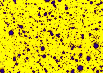
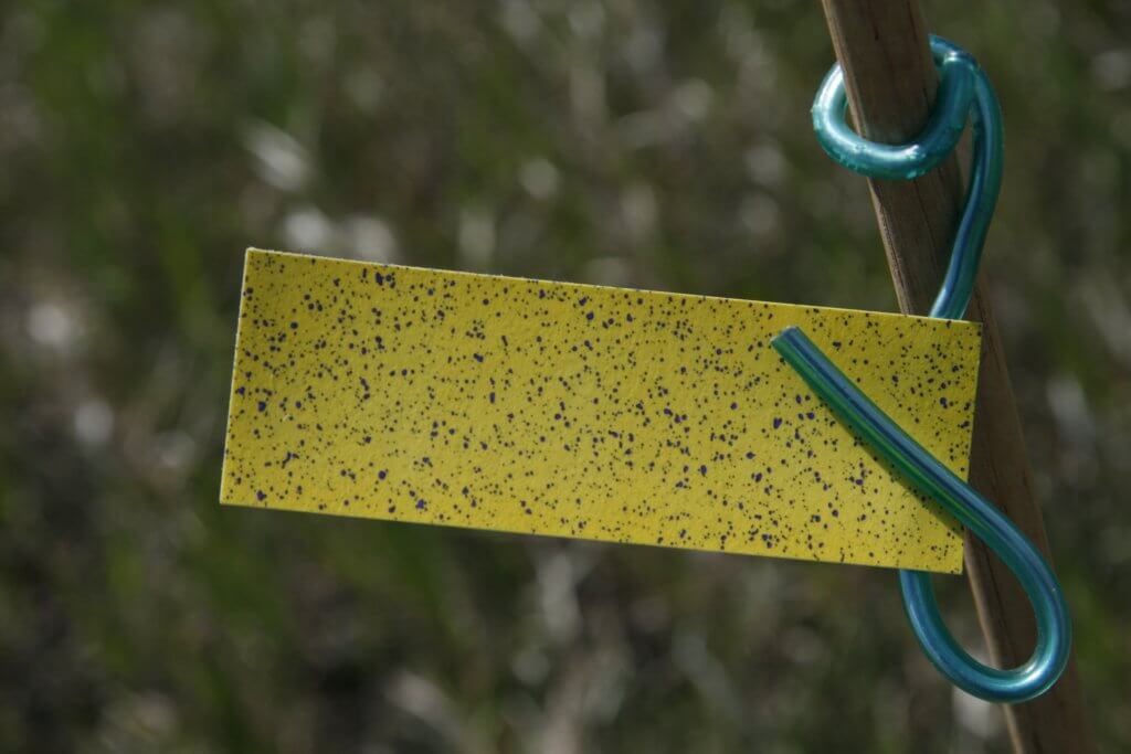
Fig. 1: Water-sensitive paper (WSP) treated with a Very Coarse spray at about 100 L/ha. Note the coalescence and overlap of some deposits.
In addition, the overall droplet density has to be low enough to avoid overlaps or coalescence. Usually a water volume over 50 to 100 L/ha will create issues. The WSP also has to collect the droplet in the first place. Smaller droplets often move around larger objects such as a leaf, or a similar sized piece of paper. If they impact at a sharp angle, the deposit will be elongated due to smearing and that creates additional difficulties.
Even if the paper collected the smallest droplets, they may not appear as stains. Droplets below a certain diameter (about 50 µm) do not leave a visible deposit on the paper.
So, while WSP is a great tool for visualizing a deposit, its limitations usually prevent it from being used to accurately measure the droplet size spectrum of a spray.
The Rise of the Laser
In the 1970s and 80s, we saw the introduction of laser-based droplet size measurements. With these, a spray simply needed to be directed into a such an instrument, and it very quickly determined the diameter, and in some cases, the velocity, of the droplets. The principles employed by various laser instruments differed, and although one could now rapidly obtain data in-situ, the numbers among the instruments didn’t always agree.
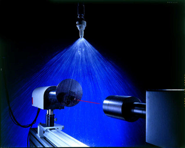
Fig 2: Laser instruments help to measure droplet size of sprays (photo source: TeeJet)
The Most Common Laser Systems
Laser diffraction: One of the first droplet sizing instruments is manufactured by Malvern (https://www.malvernpanalytical.com/en), and is still in use today. A laser beam passes through a spray cloud. The system uses a laser diffraction principle that works as follows, according to Malvern: “Large particles scatter light at small angles relative to the laser beam and small particles scatter light at large angles. The angular scattering intensity data is then analyzed to calculate the size of the particles responsible for creating the scattering pattern, using the Mie theory of light scattering.”
To calculate the droplet sizes responsible for the scattering behaviour, the laser system has light-sensitive sensors in concentric circles behind the spray plume. When a sensor in the middle of these rings picked up a signal, it likely originated from a larger droplet because of its lower light scattering properties. Sensors further from the centre picked up smaller droplets. The system thus had an idea of the relative frequency of the various droplet sizes in the spray cloud and modelled these according to the classic Rossin-Rammler spray distribution model, from which descriptive parameters are calculated.
Laser diffraction is the most popular method for in-situ droplet sizing. The company Sympatec (https://www.sympatec.com/en/) also offers a system that competes with Malvern that is found in many labs.
Laser Shadowing: The Particle Measuring Systems (PMS) system was one of the earliest laser systems. It was a very compact and sturdy system that shone a laser light at the spray cloud and the droplets in that cloud cast shadows against a sensor array a fixed distance away. The size of these shadows could then be measured to arrive at a droplet size distribution. The PMS was particularly good at measuring small droplets.
Although long discontinued, the PMS system had the basic appearance of a torpedo and was often mounted on aircraft or in wind tunnels to measure cloud aerosol sizes. Very cool. The company still manufactures other particle measuring devices (https://www.pmeasuring.com/).
Pulsed Laser Illumination: This is a different approach to the laser shadowing of the PMS system. Oxford Lasers systems (https://oxfordlasers.com/) use a video camera to view the spray cloud and freeze images from using a very high frequency pulsed laser light. This light illuminates the cloud briefly which allows a still image to be briefly displayed. Image analysis then measures the diameter of each particle in the image, adjusting for out-of-focus images. It’s possible to analyze the speed and direction of the particles by comparing the particle position in subsequent images. This system is quite popular among scientists due to its ease of use. A portable unit that can be deployed in fields is available.
Phase Doppler: In the mid 1980s, a system was developed that uses the Doppler principle to measure both the speed and diameter of droplets. Two out-of-phase laser beams intersected in a spray cloud, and a droplet passing through the intersection point created a Doppler burst that signalled the speed of the droplet. The burst signal also contained information on the droplet diameter, derived from a frequency shift of the two laser beams utilized in the system. This system has very high data acquisition and was the first to create a temporal sample of the spray, increasing the accuracy of the droplet size measurements.
Initially brought to market by Aerometrics (later acquired by TSI) and called the Phase/Doppler Particle Analyzer (PDPA), it is now mainly offered by Dantech systems (https://www.dantecdynamics.com/).
Sampling Bias: Temporal vs Spatial
It’s not straightforward to measure a sample of moving objects. It may seem intuitive that if one wants to know how many objects are present, taking a picture and counting the objects would provide the answer. But when objects move at different speeds, that answer will be incorrect because the slower moving objects will be over-represented.
Let’s assume you’re working on a traffic count project to understand the number of people crossing a bridge either walking or cycling. Let’s also assume that one walker and cyclist depart for the bridge every 5 seconds, i.e., there are the same number of each. If you wait until the bridge is full of people crossing and take a picture it will show more people walking on the bridge than riding bicycles. That is because the bicycles are faster and many will already have left the frame. Thus counting the number of people in the picture over-estimates the number of walkers because they move slower.
The same problem arises with these laser systems because in a hydraulic spray, the smaller droplets move slower than the larger droplets. Any system that takes a picture and counts what’s in it will have what’s called a spatial sample, overestimating the slower (smaller) droplets.
A temporal sample can measure the velocity of the droplets and therefore account for their speed, giving a more accurate measure of the abundance of the droplets. In the case of the PDPA, it acheives this simply by counting all the individual droplets that pass, in sequence, through its meassurement area, called the probe volume. As they pass, it notes their velocity and diameter.
To address this issue with a spatial sampling instrument, many labs now use wind tunnels and direct the spray to be tested with the wind direction. This forces the droplets to move at more or less the same velocity as the wind, eliminating or at least minimizing the speed differences before the droplets reach the laser instrument.
WSP produces a temporal sample because it ultimately catches all droplets, but it has different types of sampling bias. Large deposits usually cover smaller ones. Smaller droplets may not impact on the target due to poor collection efficiency. Small droplets may dry too quickly to leave a visible stain. As a result, even if we had accurate spread factors, we would tend to under-estimate the number of smaller droplets, opposite of the error of spatial systems.
Scanning the pattern
Droplets are not distributed uniformly within a spray pattern. In a flat fan nozzle, for example, the centre of the pattern contains the smaller droplets. The outside edges of the pattern contain fewer small droplets and more large droplets. Some laser systems have a very shallow depth of field, and the PDPA is a point-measurement. As a result, it is not accurate to simply point the measuring device at a single location of the spray pattern. Accurate droplet size spectra from lasers requires a thorough traversing scan of the spray pattern along at least its long axis, and preferably two or more such traverses at increasing distances from this central axis. The scanning method would likely need to be adjusted to suit various types of atomizers, such as hollow cone nozzles.
If no traversing mechanism is available, it is acceptable to measure the spray at several discrete locations and then merge the data prior to analysis. In all cases, three replicate samples should be taken so that an estimate of variability is available.
Many labs, having compared a full scan with many traverses to those with fewer traverses have opted for a simple back and forth traverse with little loss in accuracy.
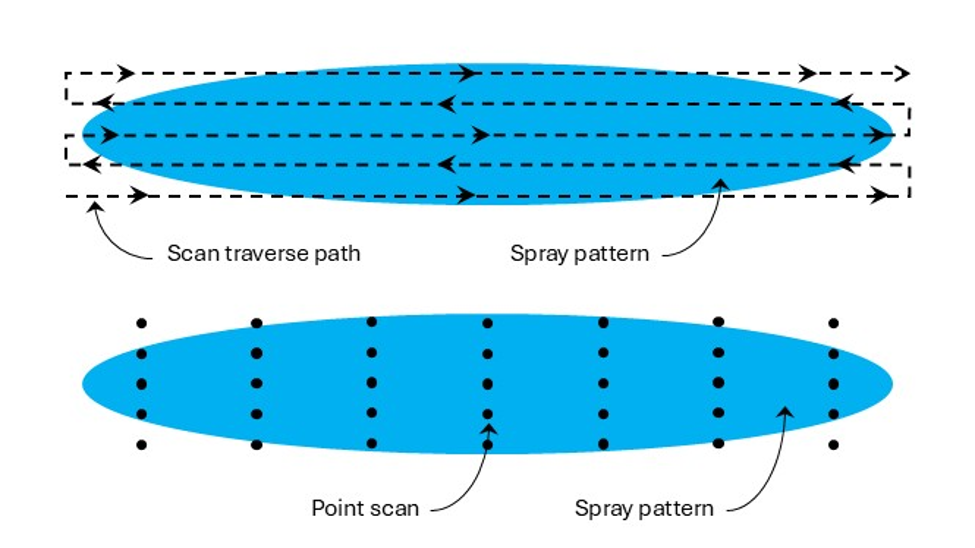
Fig. 3: Possible ways of scanning a spray pattern for droplet size analysis. Top: traversing scan. Bottom: point scan
Sometimes sprays are atomized within a chamber to prevent the droplets from contaminating the surrounding area if they contain any active ingredients. These chambers can also add measurement errors from, say, small droplets that recirculate within the chamber, or due to any glass surfaces through which the laser lights must pass. These all need to be considered, as they add to the many variables that create different results even when comparing identical sprays between labs.
The next topic, covered here, is how to use the information we gather from droplet measurements. As you might expect, this is also not as straightforward as it seems.
September 15, 2026
How to Calibrate a Drone – Swath Width Calculation
Calibration is a fundamental step in any spray application. To apply the correct product rate, we need to know how much liquid per unit land area is deposited under the sprayer.
To conduct the calculations, either manually or through the drone software, we need to know the width of the spray swath. This task requires the operation of the sprayer under typical conditions, some kind of sampler capture the spray deposit, and a means of quantifying that deposit so the spray pattern becomes apparent. Here’s how we do it:
1. Confirm the accuracy of the flow meter
Drones don’t typically report the spray pressure of the spray mix. Instead, they report the flow rate using a built-in flow meter. The drone maintains the desired application rate by using the flow rate to adjust pump speed and engage nozzles over a range of travel speeds. Because everything depends on the flow meter, its accuracy needs to be verified.
- Fill the spray tank with clean water and flush all the lines.
- Install nozzles required for task, ensuring all nozzles are identical and in good working order.
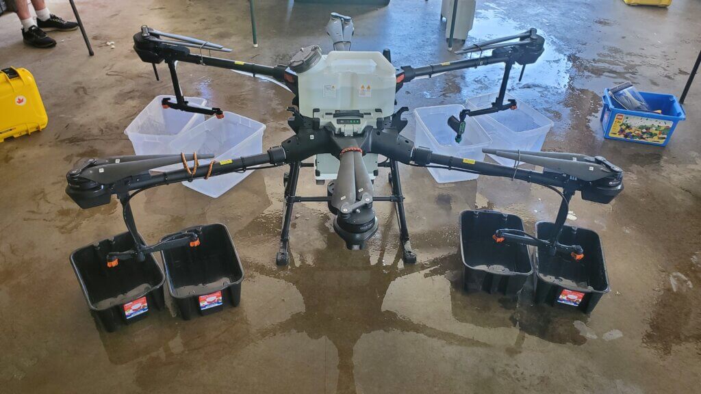
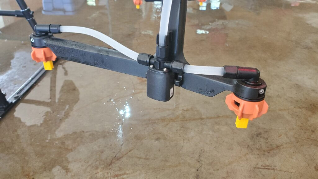
Nozzles installed on DJI T20 drone.
- Select the nozzle size you installed on the spray monitor.
- Purge the air from the system.
- Activate the spray and wait for the flow rate to stabilize on the spray monitor. This may take a few moments.
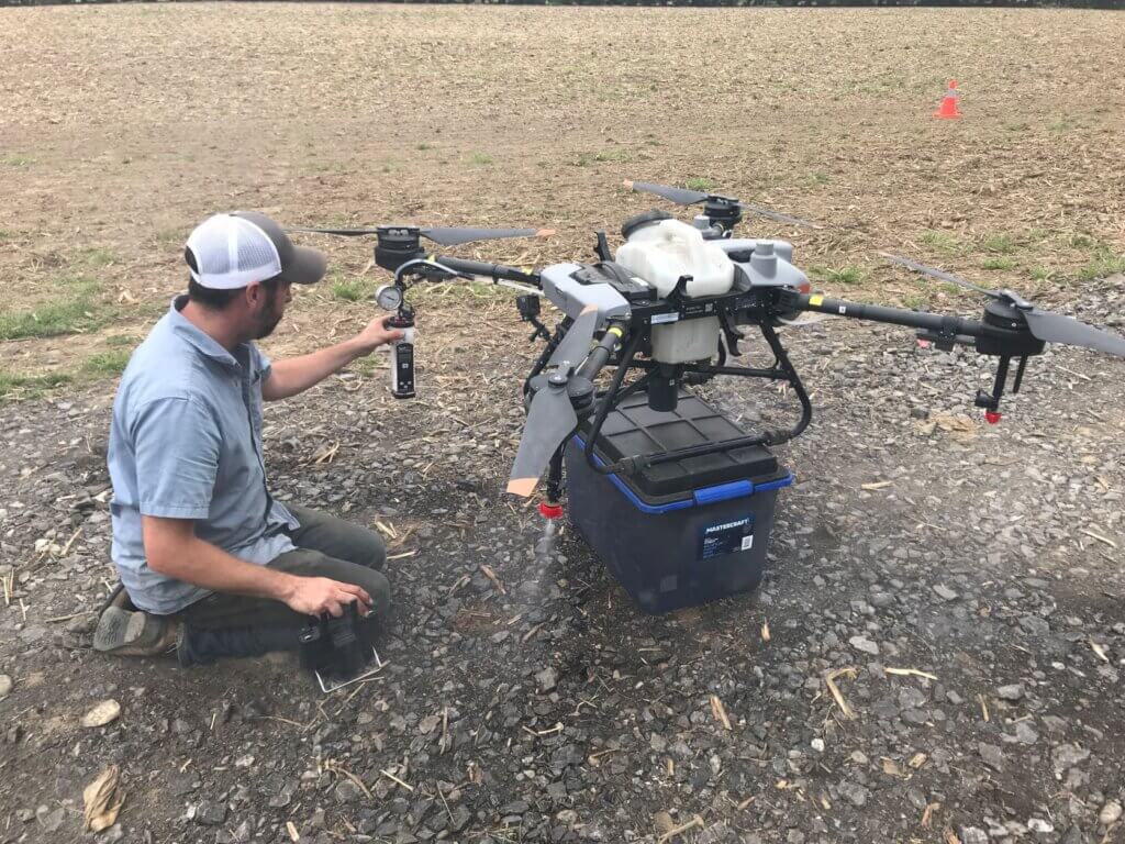
- With the nozzles flowing, place collectors under each nozzle and collect the spray liquid for a fixed time, say one minute.
Capturing spray during flow meter calibration.
- Ensure the collector catches all the spray. Buckets often create turbulence. Rotary atomizers make this more difficult.
- When the time elapses, remove the collectors and then shut off the spray.
- Unless the shutoff is very fast and positive, leaving the collectors in place during shutoff can introduce error as the flow diminishes.
- Confirm that the volume collected from each nozzle was identical, and that the flow rate reported by the drone flow meter is accurate.
- Repeat to ensure consistency.
Use of a Spot-On digital calibrating cup ensures that all spray is captured and it also reports the volume instantly.
2. Measure the swath width
Spray swath width is variable. For a measurement to be relevant we must evaluate spray deposition under environmental conditions that are similar to the planned spray operation, as well as use the same operational settings such as altitude, travel speed, nozzle choice, and application volume.
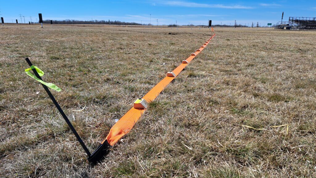
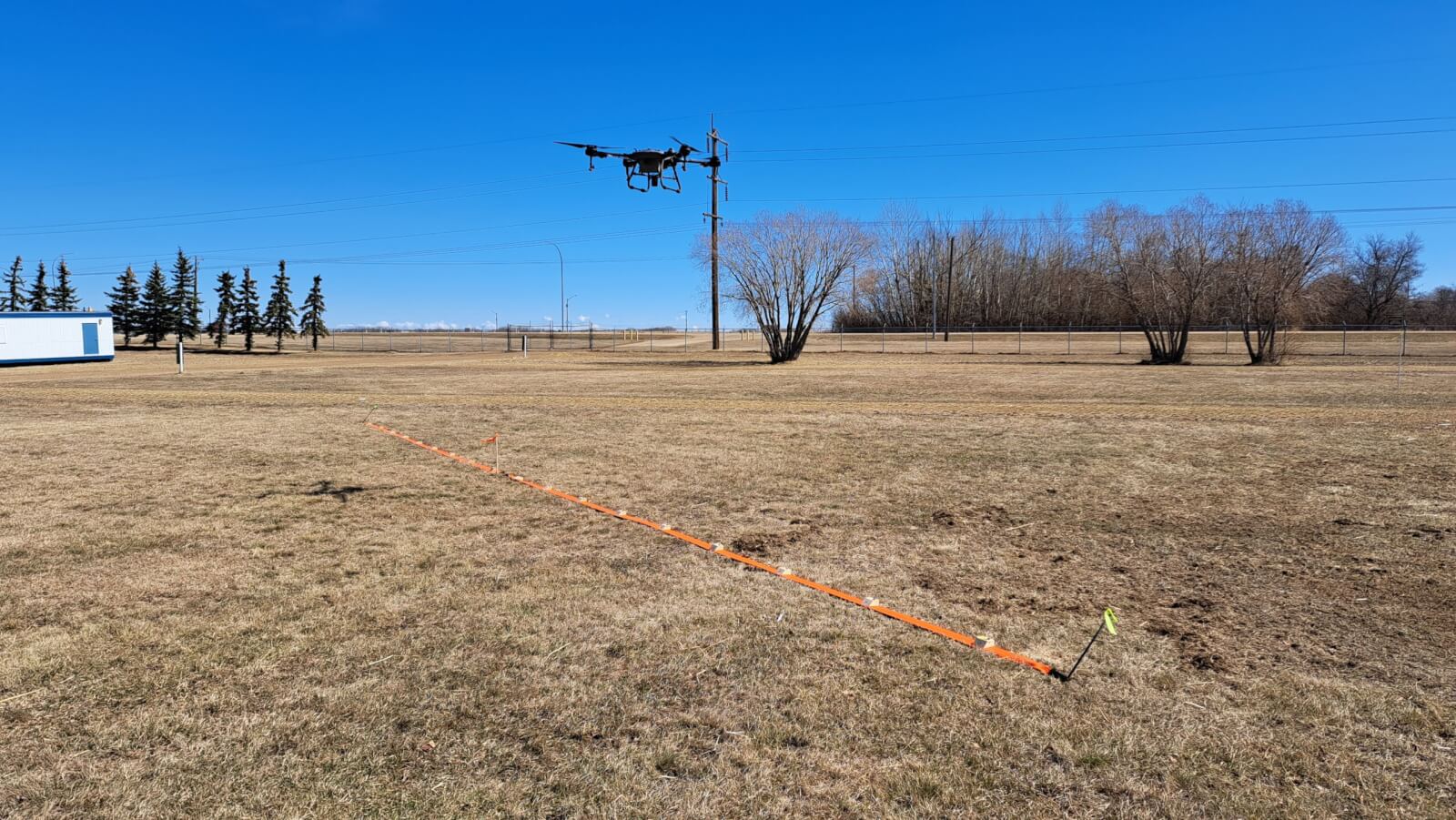
Spray samplers are positioned along the ground, perpendicular to the flight path. We use water-sensitive paper (WSP) because it’s readily available, fast and easy to use, and the deposits can be analyzed visually or using simple apps that calculate coverage. We create a sampling line of WSP positioned a 1 m intervals (or maybe 0.5 m for narrow swaths). The samplers should extend to twice the expected swath width to account for any swath displacement from sidewinds.
- Choose a day with light, consistent winds.
- Find an open space free of obstruction in the direction of the prevailing wind.
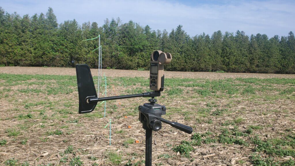
- Install a weather station to document conditions during flight.
A Kestrel 3550AG or 5550AG wind meter can record weather data and download to a phone via Bluetooth.
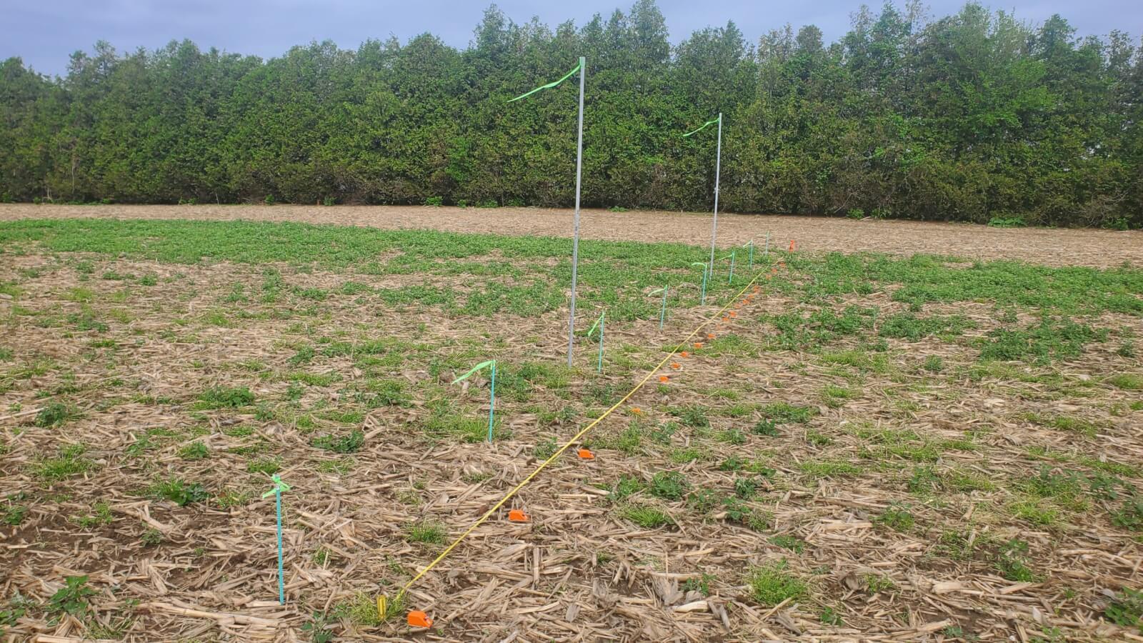
- Mark an approximately 200 m long flight line into the prevailing wind direction by placing wire flags every 50 m.
- At the 150 m mark, use wire flags to centre a sampler line perpendicular to the flight path. Sampler line length should be about twice the expected swath width.
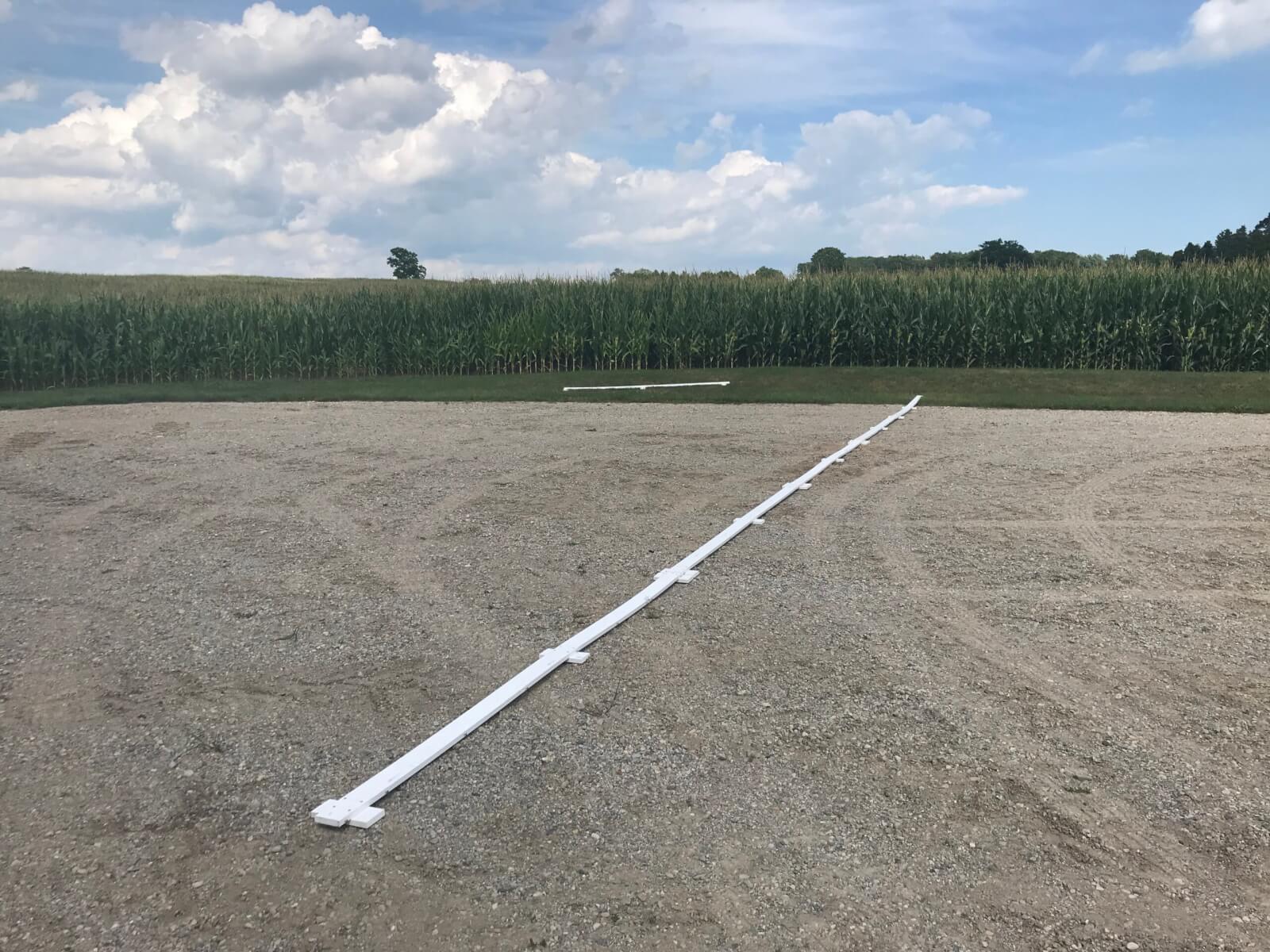
Swath sampling line
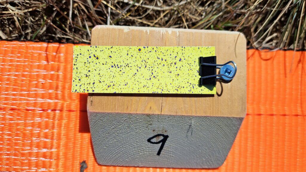
- Wooden blocks with paper clips can be used to secure WSP at regular intervals along the sampler line.
Wooden blocks attached to a 4″ tow strap allows for easy setup and movement of sampling line.
- Fill the drone 1/2 full.
- Manually fly the drone along the entire flight line. The spray pressure, flow rate and altitude of the drone should be stable before it reaches the sampler line. This may take 25 meters or more depending on drone model, flight speed and drone weight.
- Fly 50 m past the sampling line without any drone maneuvering to avoid affecting the deposit.
- Land the drone and walk along the sampler line.
- Note the deposits in the central region. Walk along line as the deposits taper off, looking for deposits that are approximately 50% of the average central deposits.
Water-sensitive paper following a drone application.
- Estimate the distance between these deposits on both edges of the swath. This is the estimated swath width that can be entered for the second flight.
- Replace the WSP with a fresh set, refill the drone to 1/2 full, and repeat the flight two more times.
Other methods perform a more advanced assessment by analyzing the entire swath, and not just intervals. These methods use dyes and dedicated hardware to quantify the deposits along strings or paper samplers.
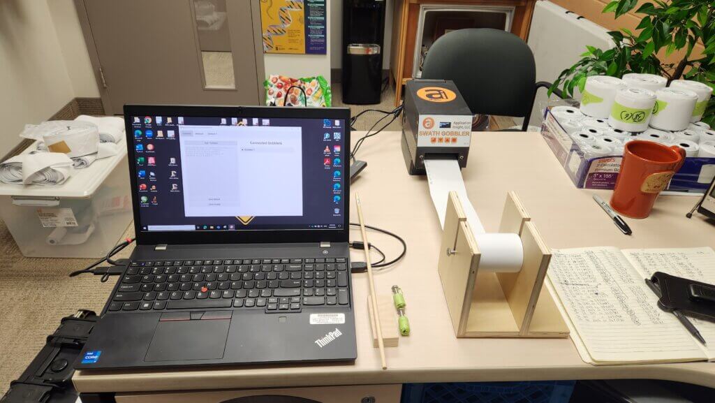
The Swath Gobbler documents swaths at high resolution using lengths of 3″ bonded receipt paper, food grade dye, and a digital scanner.
The Application Insight LLC Swath Gobbler scanner in action.
3. Analyze the Pattern
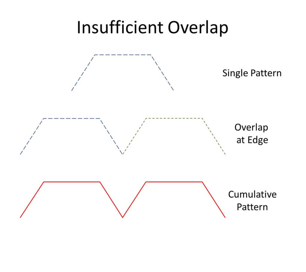
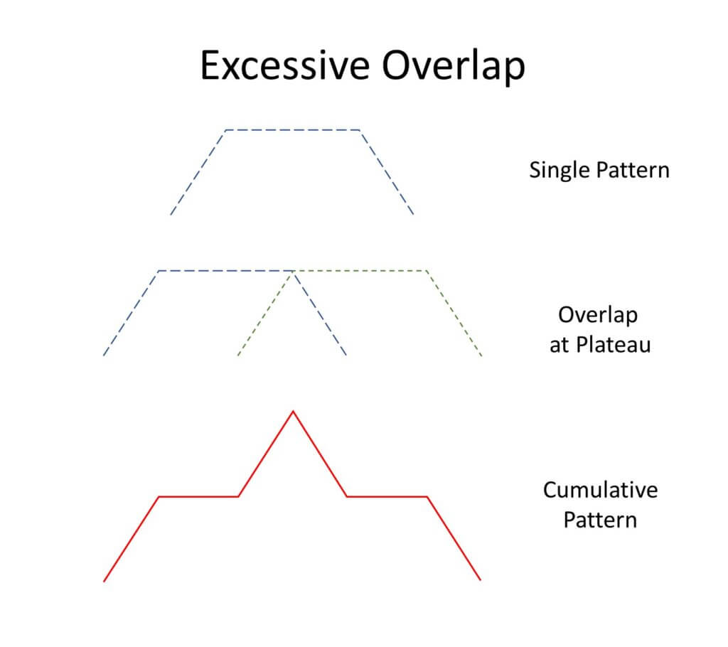
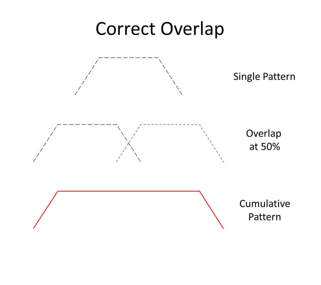
The nearest approximation for drone swathing is that of a manned aircraft. The spray pattern of an aircraft is tapered, meaning the highest deposition is near the centre of the swath, and the edges of the swath fade to zero deposit. In order to achieve consistent coverage, we need the edges of the spray swath to overlap so the cumulative coverage at the edges is closer to that in the centre. Too little overlap leaves gaps and too much overlap results in excessive deposit.
Insufficient overlap creates gaps in coverage
Excessive overlap results in over-dosing and waste
Correct overlap is necessary for efficient and effective application.
Deposits from drones can be highly variable. The challenge is to find an overlap distance that minimizes this variability, minimizes both over- and under-application, and maximizes swath width. Download a copy of an app we’ve developed to help you with this process.
swath_calculator v9 Download
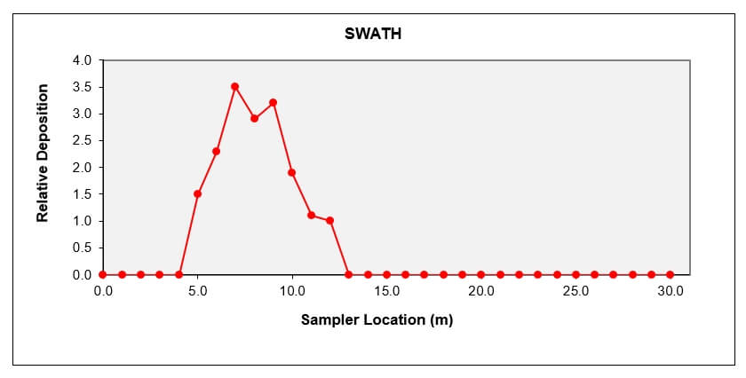
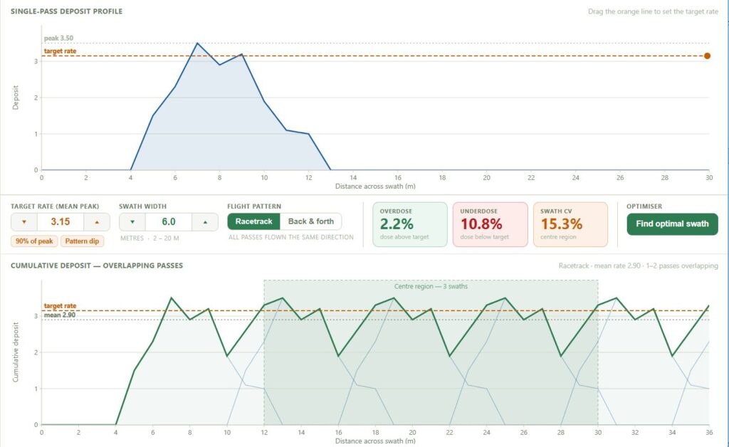
The first step is to estimate a reasonable average deposit, called “Threshold”. The app graphs the deposits from each sampler, and the user estimates a point on the Y axis (Relative Deposition) that represents the average maximum deposit. This could be the maximum value of the plateau, or a midpoint between the maximum and a nearby dip. The app assumes a value that is 90% of the maximum, to start.
We then take 50% of this estimated average deposit, and find the two distances on the X axis (Sampler Locations) that intersect the curve at these points. The distance between these two points is our first estimate of the swath width. If two adjacent swaths are spaced so the edge of one overlaps 50% with the next, the overall cumulative deposit should be relatively even.
The coverage information from each sampler location is graphed to create a deposit pattern.
We can alter the amount of overlap to improve the apparent uniformity, but be cautious. For example, even though we can often improve the uniformity by narrowing the swath width, this can add deposit to the area under the drone and raise the overall deposit amount. That would be waste. Plus, the narrower swath also lowers the productivity of the drone. Use the app to establish a swath width that has the lowest variability (Coefficient of Variability or CV) AND results in a balance between over- and under-dosing. The app has an “Optimize” button that can do this for you.
It’s possible to select a racetrack or a back and forth pattern. We’ve been using the racetrack pattern even though in real life the drone will frly back and forth, for the following reason: We expect a field to be sprayed in a sidewind. The tail of the deposit will always be on the same side of the pattern even with a back and forth flight path. In essence, the wwind creates a racetrack pattern for us.
The amount of overlap is adjusted to minimize variability (CV) and both equalize and minimize over- and under-dosing.
The app allows you to import your data using an Excel file. If the file has multiple data column, the user can select the column to be analyzed. From that point, other columns can be selected as the analysis proceeds. Each analysis can be saved and exported as a pdf file.
4. Recognize the factors that influence swath width
Operational use case affects swath width
Swath width is affected by altitude, speed, water volume and spray quality. Generally, higher altitudes, lower volumes, and finer sprays will result in a wider swath. Unfortunately, the same configuration also results in greater drift. It is recommended that swath widths be determined for each spray volume and nozzle arrangement that will be used.
Drones will be applying low water volumes and this requires a critical assessment of coverage to ensure the deposit density is sufficient to achieve the desired result. A low volume will require a finer spray for minimum coverage to be realized. Coarser sprays that reduce drift and evaporation will need higher water volumes and result in narrower swaths. Significant time may need to be invested to understand the effects of operational settings and environmental conditions on spray deposit uniformity and swath width.
Effective Swath Width and the Agronomic Use Case
The relatively sparse coverage at the extremes of the measured swath width may be insufficient to elicit the desired biological result. The Effective Swath Width (ESW) represents the segment of the total swath width that results in pesticide efficacy. In some use cases, the two widths can be similar, but typically the ESW is only a fraction.
The difference is influenced by the “Agronomic Use Case” which includes factors such as:
- Spray mix rheology (i.e. the interaction of spray mix viscosity and atomizer design on droplet size)
- Minimum effective dose: This is a complex relationship between coverage, spray mix concentration and pesticide mode-of-action that results in an effective result while minimizing the environmental impact.
- Target location (e.g. a pest within a dense canopy or a weed on relatively bare ground)
Taken collectively, research has shown a 20-30% reduction in ESW for corn, wheat and soybean fungicide applications compared to swaths measured on open ground. Conversely, herbicides sprayed on bare earth or sparse vegetation can produce an efficacious response 20% wider than the measured swath width. The impact of agronomic use case on ESW must be considered during mission planning.
Additional pointers
Here are a few tips and tricks to help you be successful when calibrating your drone.
- Drone patterns will have deposit peaks and valleys in the central region. Repeated runs are needed to confirm that these are real and persistent. If so, then adjustments in flying height, spray quality, or water volume may be needed to eliminate them.
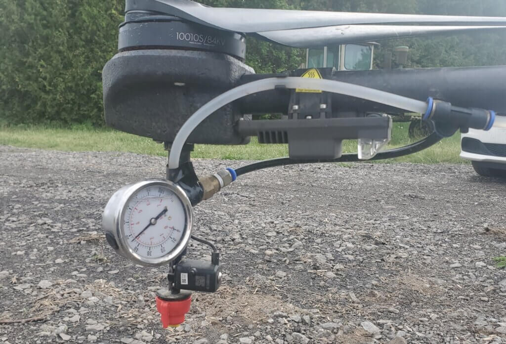
- The absence of pressure gauges on drones can be corrected by installing an analog gauge in-line with one of the spray nozzles. If may be necessary to mount an auxiliary camera on the drone to record this gauge. We have observed strong fluctuations in spray pressure, particularly on starting a spray swath, that were not reflected in the reported flow rate.
A pressure gauge can be plumbed into a drone without affecting flight behaviour. A camera is trained on it to read pressure during a flight.
- Many drones have the option of recording the flight screen during a mission. This will provide a record of the performance of the drone, and can be valuable should performance problems arise.
- Although swath width calibration is done by flying into a headwind, the actual spray application should be done with a side wind. Start at the downwind edge of the field and turn into the wind. The drone is symmetrical and the tapered spray patterns should equalize the deposits. Alternately, flying into a headwind and returning with a tailwind can alter the aerodynamics of the spray deposition process, alternating between a wider and more narrow swath width, respectively.
Drone spraying will walk a razor’s edge of sorts – there is little room for error when using scant water and fine droplets. Getting the basics right has never been more important.
September 12, 2026
How Much Pesticide in the Tank?
Sprayer math can be intimidating, but the effort gives solid value. When combined with a calibrated sprayer you reap the following benefits:
- Determine how much spray mix is required to apply the intended rate.
- Estimate how much crop protection product must be ordered for the season.
- Populate spray records which allow you to review practices, respond to enquiries and satisfy traceability requirements.
There are many ways to perform sprayer math, and you need only look to local pesticide safety courses, industrial catalogues, and extension resource centres for examples. If you’re already comfortable with your current method, don’t mix and match with others. Sprayer math is a series of related calculations that employ constants to keep the units straight. It’s all or none.
Walkthrough
Let’s start with the classic, US Imperial formula for calculating the sprayer output. We’ll weave in Metric, later. This base formula can be adjusted to allow you to solve for any factor, as long as you’re only missing one piece of information. Turns out your high school teacher was right – you DO need algebra.
GPM = [GPA x MPH x W] ÷ 5,940
In this case, you can determine an output rate (GPM – gallons per minute). You’ll need to know your target volume (GPA – gallons per acre), your average travel speed (MPH – miles per hour) and your nozzle spacing (W – which is width in inches). The number “5,940” is a constant that handles all the unit conversions. If you divide the GPM by the number of nozzles on your sprayer (assuming they are all the same rate), you can hone in on the ideal nozzle size.
But, as we noted earlier, you can do a lot more with sprayer math than just pick the ideal nozzle size. The rest of this article includes examples of both Metric and US Imperial formulae, but watch out for unit conversions. If at any time you don’t see the units you’re looking for, you can consult our unit conversion tool.
Grab your calculator – it’s math time!
Don’t be intimidated. With a little practice, sprayer math gets easier and it’s always worthwhile. The real trick is navigating unit conversions.
Step 1 – How large is the area you need to spray?
Multiply the length of the area you plan to spray times the width. If you are using metres, then divide the product by 10,000, which is the number of m² in a hectare (ha). For feet and acres, divide by 43,560 which is the number of ft² in an acre (ac):
Step 2 – How much product is needed to spray the area?
Consult the rate(s) shown on the label. In Canada, rates are often based on planted area (E.g. hectares). In Australia and New Zealand, they may be based on row length (not covered in this article). If you measure your area in acres, you’ll have to convert the rate by multiplying by a constant: 0.4.
Now multiply the area you want to spray (step 1) by the rate (step 2).
Step 3 – How far can you go on a full tank?
You know your sprayer output (determined through calibration) so you divide that into your tank size. Watch your units:
Step 4 – How much pesticide per tank?
Multiply the area that can be sprayed per tank (Step 3) by the pesticide rate (Step 2). Again, watch your units:
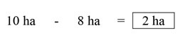
Step 5 – How much area is left to spray?
Just subtract what you’ve already sprayed from the total area.
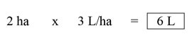
Step 6 – How much pesticide in the last, partially-full tank?
Multiply the area you have left to spray (Step 5) by the pesticide rate (Step 2). Yes, watch your units:
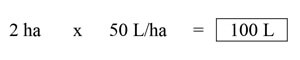
Step 7 – How much spray mix will I need for the partial tank to finish spraying the total area?
Multiply the area you have left to spray (Step 5) by the sprayer output (determined through calibration). Guess what? Watch your units:
Sample problems
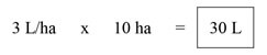
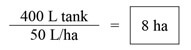
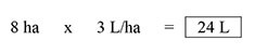
Time to test your knowledge. Let’s suppose you want to apply a product rate of 3 L/ha to your blueberries. You calibrate your sprayer and determine your output to be 50 L/ha. Your tank holds 400 L of spray mix. Your planting is 500 m long and 200 m wide.
Q1 – How large is the area you need to spray?
Q2 – How much product is needed to spray the area?
Q3- How much area can be sprayed on one tank?
Q4 – How much product should be added to a full tank?
Q5 – After the tank is empty, how much area is left to spray?
Q6 – How much product to add to the last, partially full tank?
Q7 – How much spray mix will be needed to finish spraying?
Tank mix calculator
You might feel we buried the lead by adding this calculator to the end of the article. It’s important for a sprayer operator to understand the math required to interpret labels and calculate tank mixes, so hopefully you read and understood the process before you got here. And now that you have, this is a very helpful tool. Try it online, or download a standalone version.
Notable exceptions
Certain situations aren’t covered in this article. If you are spraying a greenhouse, the math is different. If you are performing a banded application, the math is different. And, if you’re an airblast operator trying to reconcile why a pesticide label uses planted area rather than canopy volume for its rates, you’re in for some additional reading.
September 9, 2026
The Ultimate Sprayer Calibration and Unit Conversion Tool
Canada, like most of the world, is officially Metric. America operates using the US Imperial system. It sounds very cut and dried, doesn’t it?
However, anyone that’s tried to calibrate a sprayer in Canada quickly discovers that we’re really an amalgam of the two systems. We like to call it “Mock-tric“. By way of evidence, some operators still adhere to the dreaded L/ac. You know who you are. To be fair, some of our sprayers and nozzles originate from the states, meaning nozzle tables and rarely, sprayer indicators, can be in US Imperial.
This leads to mind-bending questions such as:
I drive 12 mph, spraying 150 L/ha and my pressure is about 40 psi. How many ml/min should my 72 nozzles emit for a product that wants a 6 oz/acre acid equivalent?
Cue the quiet sobbing…
Frustrated back in 2017, we created a set of conversion tables to help operators with almost any Imperial/Metric emergency. Admittedly, they were in 4-point font and therefore too cumbersome for practical use. We’ll keep one here for posterity.
The good old days of “look-up tables”. RIP.
Happily time has marched on and we now have a better way. Explore our new Sprayer Calibration and Unit Conversion Tool, below. While it doesn’t do it all, it certainly does a lot! You can:
- Convert between common (and some uncommon) agriculturally-relevant units.
- Calibrate a field sprayer for both broad acre or banded applications.
- Calibrate an airblast sprayer for almost every traffic pattern and swath width.
- Calibrate a plot sprayer, either for a handheld boom (any number of nozzles) or for a backpack sprayer mist/wand in 3D rows.
- Calibrate a fogger for common closed environment structures
To use this suite of calculators correctly, the user needs some agronomic understanding of what these variables mean and how to obtain them. In order to provide context, and reduce the friction, we’ve added a link to relevant articles at the top of each calculator.
Grab an offline version here, or try it out below. We’ve tried to validate every path, but if you find a bug, please let us know. Once you know your calibration settings, go here to determine how much goes in the sprayer tank.
September 4, 2026
We Need Better Drift Control Technologies
Sprayer manufacturers have all but offloaded the entire responsibility for drift management to the sprayer nozzle. It’s asking too much.
Sprayers have changed a lot over the past 25 years. They have become larger, with more tank capacity, boom width, and, if self-propelled, horsepower. They are more comfortable and ergonomic, with more sophisticated swath control and guidance systems. But every year, a very important deficiency in their design becomes obvious. Drift control.
The changes described above are intended to improve productivity and fight operator fatigue. Today’s sprayer can cover more ground than ever before. But the demand to cover ground, through a combination of growth in farm size and frequency of treatment, has outpaced machine productivity. As a result, operators find themselves ever further in a time deficit, with acres on the to do list and no time to get the work done.
Spray drift remains the single most limiting factor to the safe application of pesticides. Spraying cannot happen when it’s too windy or during inversions because all agricultural nozzles produce fine droplets whose movement in the atmosphere cannot be controlled. This has been an issue since spraying began.
Simply put, pesticides belong in one place only, and that is on the treated swath. Applicators have some tools to make this happen, such as using coarser sprays, lowering the booms, choosing very specific weather conditions, and the like. But when winds are incessant, and crops and pests are quickly growing out of the treatable stages, what is an applicator to do? There is only one thing they can do: lower their standards. Either miss the treatment and suffer the yield loss, or spray in the wind and hope nothing bad happens.
Neither of these options are acceptable.
There isn’t an easy fix. Spraying is a game of tight margins. The spray liquid in the tank must be atomized into droplets that can make their way to the target and provide adequate coverage when they get there. The total liquid volume to achieve that task must also be practical. The global ag industry has determined, over the past 100 years, that about 100 to 200 L/ha, 10 to 20 gallons per acre, is the ballpark amount that allows reasonable work rates with sprays that are just coarse enough to resist displacement in modest winds. If it gets windier and we need even coarser sprays, we need to add more water to maintain an acceptable droplet density on the targets. And of course, the droplets need to stick to those targets, so there is a limit how coarse we can spray.
Over the past 20 years, we’ve been asking the low-drift nozzle to do the heavy lifting in drift management, and it has served us well. But with a return to more contact modes of action for resistance management, there’s a need to retain good coverage for product performance.
What ag needs is a drift-reducing technology that is better than the low-drift nozzle. We need a technology that maintains a practical water volume limit and combines this with intermediate spray qualities that generate good pesticide efficacy without allowing drift under windy conditions.
These technologies need to do just one of three things: (a) Protect the driftable droplets from exposure to moving air with a physical barrier, (b) make driftable droplets less drift-prone by increasing their velocity, or (c) eliminate the driftable droplets altogether.
Let’s have a look at some options, and explore the pros and cons.
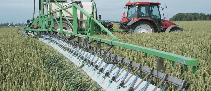
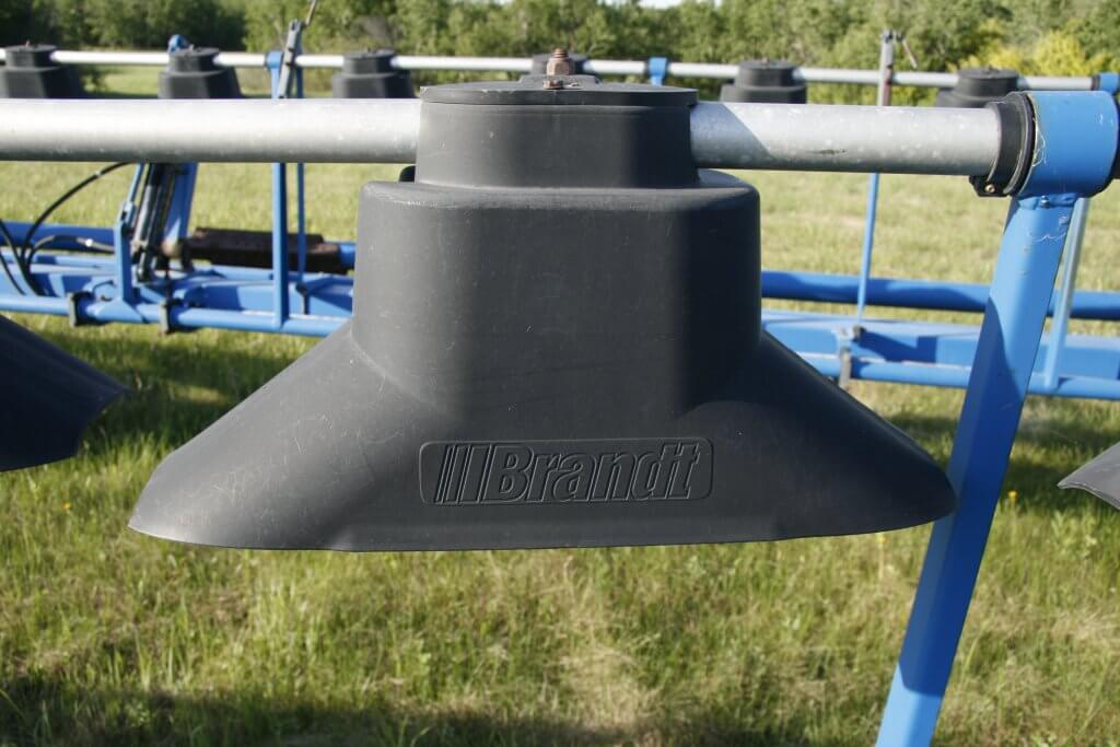
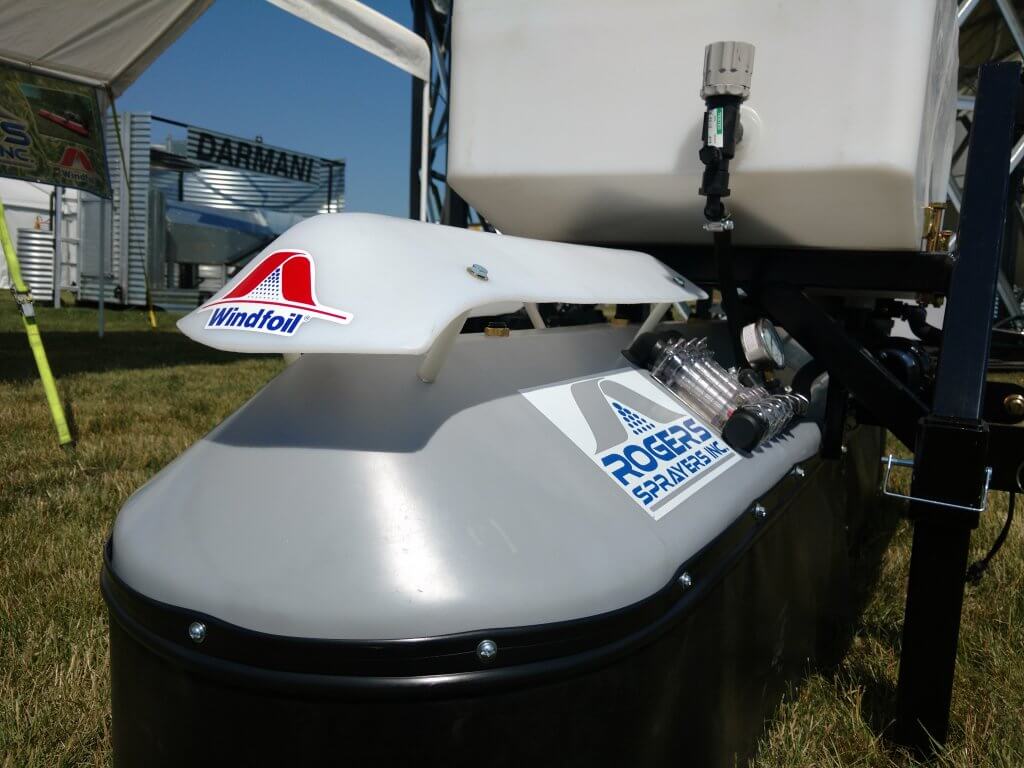
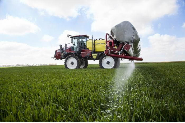
Shields and Cones. A shroud surrounding the boom was first proposed and built in the 1950s in the UK by Dr. Walter Ripper. Although never commercial, his “Nodrif” boom inspired an entire industry that took hold in western Canada in the 1980s and 1990s. Shrouding worked. In studies conducted at Ag Canada, shrouds produced by Flexi-Coil, Rogers Engineering, AgShield, and Brandt reduced drift by up to 80%. But shrouds disappeared in the 90s, partly because of the advent of tight-folding suspended booms where their physical size posed a problem, but also because of crop contamination from the shrouds and poor nozzle visibility in case of blockages.
The advent of the air-induced low-drift nozzle offered an alternative, but coarseness has been taken to its practical limit.
What about a newly engineered version of shrouds that addresses its shortcomings? Willmar Fabrication has created the Redball Buffer Sprayer, for example. We see hooded sprayers in row crops. But there may be other ideas. The simple device called the PatternMaster introduced by KB Industries a few years back was also a step in that direction. Let’s keep working on this.
Figure 1: Shrouded booms, once common on the prairies and proven effective (Brandt cones, top), are still used on research and turf sprayers (bottom).
Air Assist. Small drops don’t drift just because they’re small. They drift because they have very little kinetic energy, and they get blown off course easily. Speed them up, and that problem is solved. Introducing an air stream at the nozzle can do just that. Furthermore, air assist also enhances canopy penetration, a problem that we currently attempt to address with the addition of more water. Again, this idea is not new. Hardi, once the world’s largest sprayer manufacturer, has had the TwinForce boom available for decades. An inflatable bag is positioned over the boom. Openings along the bottom direct the air down. The operator turns a knob in the cab to control fan speed, and another for forward or backward angle, until the combination is suited to the canopy and the travel speed. The SprayAir, out of Carseland, AB (purchased by Miller but no longer available) was a less elegant version because they chose an air-shear atomizer that sometimes required more air than was prudent. Too much air rebounds off the ground, increasing the drift issue. Their Trident boom, allowing a hydraulic nozzle to be used with air assist, continues to have potential.
Air bag type air assist systems were also available from other manufacturers, but none were ever commercially successful.
Figure 2: Air assisted booms such as this Hardi TwinForce accelerate small droplets, reducing their drift-potential and improving canopy penetration (Source: Hardi Sprayers)
Low Booms. How low can booms go? It depends on the nozzle spacing and fan angle. Horsch claims that with a good boom package, this is an option. They are offering 10” spacing, and with wide fan angles, booms as low as 15” would still provide good overlap. Hands up who will try this at 18 mph. Wingssprayer has an interesting design where the boom rests on backswept plastic sheets, providing a physical barrier and a low height.
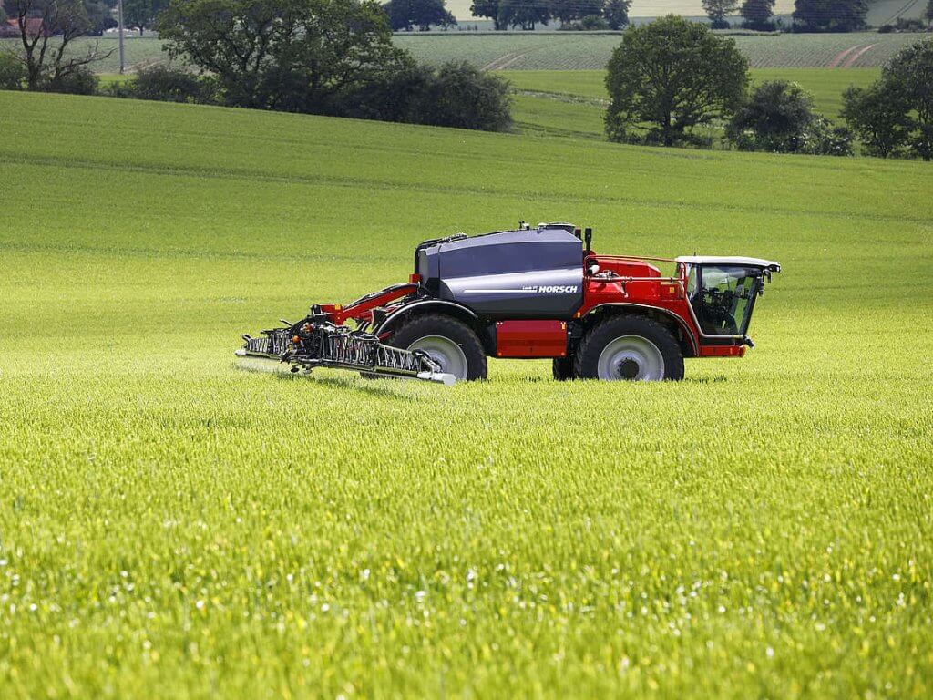
Figure 3: Low booms can significantly reduce drift, but their success depends on superior stability and height control (Top, Source: Horsch Sprayers; Bottom, Source: Wingssprayer)
Twin Fluid Atomizer. In this atomizer type, both air and liquid are forced out through the same nozzle. The ratio of air and liquid determines the liquid flow rate and the degree of atomization. First introduced by Cleanacres in the UK as the Airtec, improved by Harry Combellack in Australia over many years, and making a re-appearance with the Dutch manufacturer Agrifac, it’s been one of my favourite atomizers. The small amount of air moving through each nozzle is not enough for serious air-assist, but the idea is good and perhaps it can be improved.
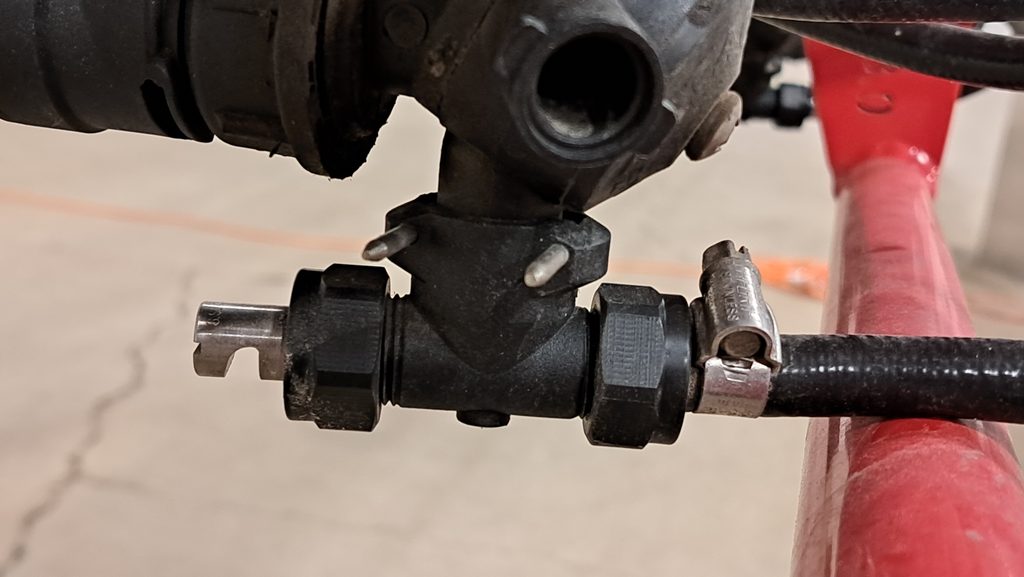
Figure 4: A twin fluid atomizer utilizes air (entering from hose) and liquid (entering from boom) to create a spray whose droplet size and flow rate are adjustable. Air generates some assist to reduce drift.
Electrostatics. Forget about it for drift control. The attractive force is so weak that it only works for very small droplets over short distances. It needs air-assist to work properly. See point #2.
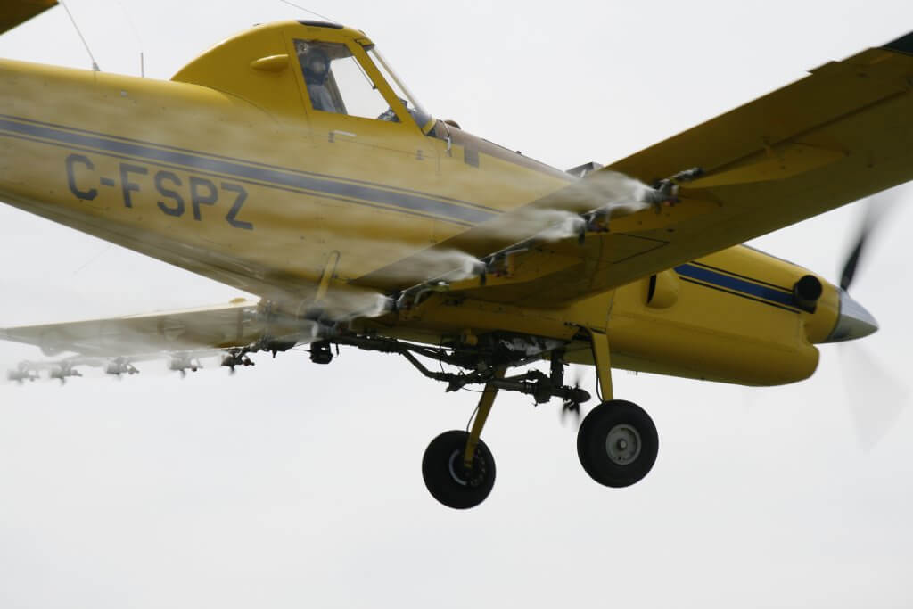
Rotary Atomizer. These are common on aircraft these days, as rotary cages, offering a more consistent droplet size range that eliminates the largest, water-wasting droplets, and curtails many of the smallest droplets produced by hydraulic atomizers. These attributes are powerful and address the fundamental problem: If the small droplets drift, then let’s not produce them. In reality, rotary atomizers are used mainly to produce smaller droplets to save water in the aerial business, not really solving the drift problem. In the 1970s and 80s, the concept was advanced by Micron Corporation, led by Ed Bals and later by his son Tom. Although very successful in forestry and hand-held applications in arid regions where water posed a serious limitation, the transition to boom spraying never happened.
Rotary atomizers are now making a comeback with drone sprayers. Though promising, the flow rate capabilities of spinning disks are lower than those of the cages mounted on crewed aircraft. As a result, the disk may flood, and will no longer produce the desired monodisperse distributions.
Figure 5: Rotary atomizers can eliminate larger droplets and sharply reduced the smallest ones, leaving a more uniform sized distribution (insert). They are used on aircraft to save water, but have not been adopted on ground equipment to control drift.
A new Atomizer. All hydraulic nozzles produce a wide variety of droplet sizes, and that variety has provided robust performance over a wide range of conditions. But it can also be a problem. Even the venerable dicamba nozzles that create Extremely Coarse and Ultra Coarse sprays produce some fines that drift in inversions. The idea put forth by Ed Bals, to eliminate the problematic size ranges, is sound. But the rotary atomizer is hard to implement on a boom sprayer. Can there be an innovation that maintains a simple overall design, produces a narrow, but low-drift droplet size range, and mates it to a bit of air assist to get the spray where it belongs? Absolutely.
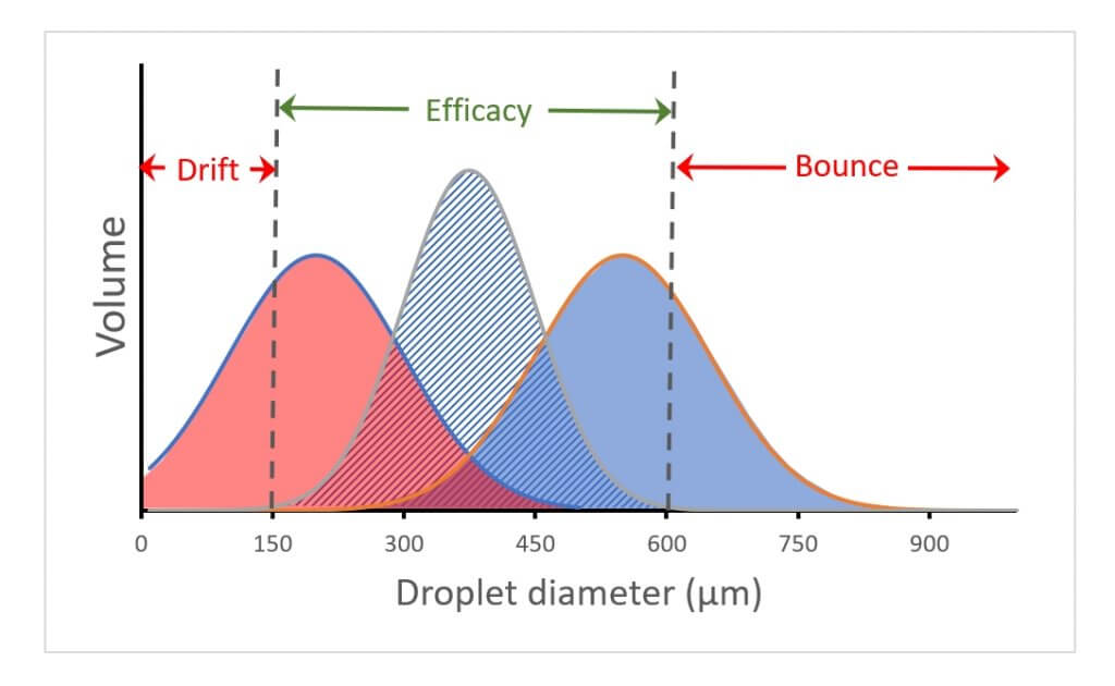
Figure 6: Current hydraulic atomizers tend to produce a wide range of droplet sizes. The distribution on the left results in significant drift (droplets <150 µm). The one on the right wastes the larger droplets (droplets >600 µm. The narrower span in the centre distribution avoids these problem areas and delivers the spray in an efficacious portion.
Adjuvants. One of the problems with low-drift nozzles is their tendency to generate some very large droplets. These droplets are not very abundant and therefore don’t contribute to coverage, but they nonetheless consume significant carrier volume. The current generation of oil-based drift-reducing adjuvants (DRAs) have helped reduce the drift-prone size fraction without increasing the largest droplet size fraction as much as low-drift nozzles do. This more surgical approach is welcome. Unfortunately, the drift-reducing effect is not as much as low-drift nozzles alone can achieve. A combination of these two technologies is likely the best way forward.
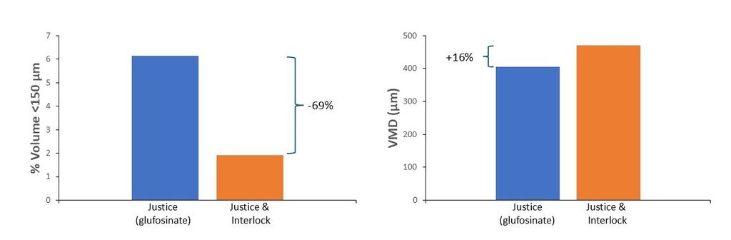
Figure 7: Effect of DRA on driftable fines (left) and overall volume median diameter (VMD, right) from AIXR11004 tip. Data courtesy Winfield United.
Targetted Sprays. An obvious way to reduce drift is to spray less. With recent developments in camera-driven spot spraying, this is already happening. It’s safe to assume that every percentage not sprayed is an equivalent reduction in drift potential. And with reports of 50 to 90% savings, this will be significant. How these product savings are deployed remains important. Some applicators choose to raise pesticide rates to effect better control, and this of course negates some of the gains. Others are increasing the overall spray volume. This then opens the door to the use of coarser sprays without loss of coverage, enhancing gains.
Figure 8: Spot spraying (Courtesy Croplands)
To create value for farmers you first need to understand farmers’ priorities and problems. Getting the spraying job completed on time often means squeezing the work into ever narrower time frame, between rains, between winds in the afternoons and inversions that same evening, between too much dew and too dry, between too early and too late. I am looking forward to the day when engineering resources are allocated to address these issues better, protecting both the environment and the stress levels on the farm.
August 20, 2026