Sprayer math can be intimidating, but the effort gives solid value. When combined with a calibrated sprayer you reap the following benefits:
Estimate how long a job will take.
Estimate how much spray mix is required.
Estimate how much crop protection product must be ordered for the season.
Populate spray records which allow you to review practices, respond to enquiries and satisfy traceability requirements.
There are many ways to perform sprayer math, and you need only look to local pesticide safety courses, industrial catalogues, and extension resource centres for examples. If you’re already comfortable with your current method, don’t mix and match with others. Sprayer math is a series of related calculations that employ constants to keep the units straight. It’s all or none.
Walkthrough
Let’s start with the classic, US Imperial formula for calculating the required nozzle output. In other words, you want to know which nozzle size you need to get the volume-per-planted area you’re aiming for. This is the bread-and-butter formula that seems to be needed most often, so that’s why we list it first.
In order to determine nozzle size (gallons per minute), you’ll need to know your target volume (gallons per acre), your average travel speed (miles per hour) and your nozzle spacing (in inches). The number “5,940” is a constant that handles all the unit conversions. It is what it is.
GPM = [GPA x MPH x W] ÷ 5,940
Of course, this formula can be adjusted to allow you to solve for any factor, as long as you’re only missing one piece of information. Algebra is all about solving for X, or in other words, determining some unknown variable. I know, it’s been a long time since you learned this in school and it doesn’t come easily to most. I propose brushing up on the basics using a series of three great YouTube videos from “Mathantics“
As we noted earlier, you can do a lot more with sprayer math than just pick the ideal nozzle. But before we continue, a warning: If you live where units are strictly US Imperial, or strictly Metric, then Canada’s odd hybrid “Mock-tric” units can get a little confusing. The rest of this article attempts to be globally-relevant by including examples of both Metric and US Imperial formulae, but watch out for unit conversions. If at any time you don’t see the units you’re looking for, you can consult our exhaustive list of unit conversion tables.
Grab your calculator or favourite smart phone app – it’s math time!
Don’t be intimidated. With a little practice, sprayer math gets easier and it’s always worthwhile. The real trick is navigating unit conversions.
Step 1 – How large is the area you need to spray?
Multiply the length of the area you plan to spray times the width. If you are using metres, then divide the product by 10,000, which is the number of m2 in a hectare (ha). For feet and acres, divide by 43,560 which is the number of ft2 in an acre (ac):
Step 2 – How much product is needed to spray the area?
Consult the rate(s) shown on the label. In Canada, rates are often based on planted area (E.g. hectares). In Australia and New Zealand, they may be based on row length (not covered in this article). If you measure your area in acres, you’ll have to convert the rate by multiplying by a constant: 0.4.
Now multiply the area you want to spray (step 1) by the rate (step 2).
Step 3 – How far can you go on a full tank?
You know your sprayer output (determined through calibration) so you divide that into your tank size. Watch your units:
Step 4 – How much pesticide per tank?
Multiply the area that can be sprayed per tank (Step 3) by the pesticide rate (Step 2). Again, watch your units:
Step 5 – How much area is left to spray?
Just subtract what you’ve already sprayed from the total area.
Step 6 – How much pesticide in the last, partially-full tank?
Multiply the area you have left to spray (Step 5) by the pesticide rate (Step 2). Yes, watch your units:
Step 7 – How much spray mix will I need for the partial tank to finish spraying the total area?
Multiply the area you have left to spray (Step 5) by the sprayer output (determined through calibration). Guess what? Watch your units:
Sample problems
Time to test your knowledge. Let’s suppose you want to apply a product rate of 3 L/ha to your blueberries. You calibrate your sprayer and determine your output to be 50 L/ha. Your tank holds 400 L of spray mix. Your planting is 500 m long and 200 m wide.
Q1 – How large is the area you need to spray?
Q2 – How much product is needed to spray the area?
Q3- How much area can be sprayed on one tank?
Q4 – How much product should be added to a full tank?
Q5 – After the tank is empty, how much area is left to spray?
Q6 – How much product to add to the last, partially full tank?
Q7 – How much spray mix will be needed to finish spraying?
Exceptions
Certain situations aren’t covered in this article. If you are spraying a greenhouse, the math is different. If you are performing a banded application, the math is different. And, if you’re an airblast operator trying to reconcile why a pesticide label uses planted area rather than canopy volume for its rates, you’re in for a lot of additional reading. Some of that latter process can be summed up in this infographic:
When you find a method that works for you, write it down and keep it with your spray records. Happy spraying!
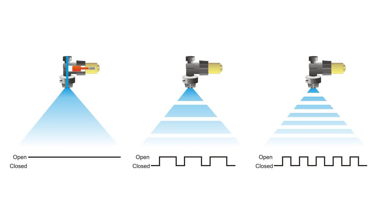
There’s a certain deer-in-headlights expression that creeps onto a sprayer operator’s face when we discuss nozzle selection. We sympathize with our field sprayer clients given the variety of brands, styles, flow rates and spray qualities they must choose from. And PWM has made the process even more complex. However, airblast operators face an additional challenge; Unlike horizontal booms, vertical booms often distribute the flow unevenly to reflect relative differences in the distance-to-target and the density of the corresponding portion of target canopy. We discuss the broader, iterative process of nozzling an airblast boom here, but in this article we focus on the topic of flow distribution.
An overwhelmed operator trying to nozzle a boom.
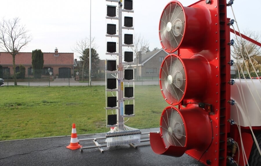
The question of “which rate goes where” is still debated. It’s led to diagnostic devices called Vertical Patternators which show the profile of the spray. Operators can use these to visualize their distribution… but they are few and far between. For the rest of us, deciding on the best distribution begins with understanding how the practice evolved.
The AAMS vertical patternator. The mast moves back and forth across the swath of a parked sprayer. Each black collector intercepts the spray at different heights. The fractions collect in the tubes at the bottom to show relative volume.An OMAFRA-built vertical patternator. The sprayer parks in front of the screens, which intercept spray. It’s collected in troughs and runs into columns that show relative volume.
1950s
In the 1950s, the mantra was to blow as much as you could, as hard as you could, and hope something stuck. At the time, John Bean promoted a method called “The 70% Rule” whereby operators used full-cone, high volume disc-core nozzles to emit the vast majority of the spray from the top boom positions. John Bean provided a slide-rule calculator to help operators configure booms to align the top nozzles with the deepest, densest portion of the 20-25 foot standard trees they were trying to protect. Back then, most airblast sprayers were engine-driven low-profile radial monsters capable of blowing to the tops of those trees. The practice persisted into the 60s and was encouraged by Cornell University (Brann, J.L. Jr. 1965. Factors affecting the thoroughness of spray application. N.Y. State. Arg. Exp. Sta. J. paper no. 1429).
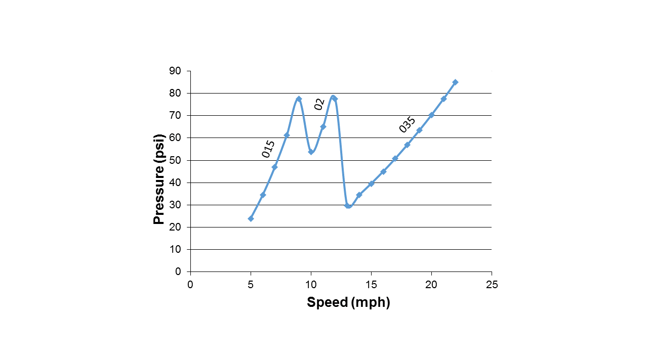
The profile of the spray would have looked something like the following graph:
1970s
In the 70s, extension specialists began advising operators to tailor the distribution to match the orchard spacing, tree architecture, canopy density and weather conditions. we reached deep into our archives for the Ontario Ministry of Agriculture and Food’s 1976 publication entitled “Orchard Sprayers” to see what we used to tell airblast operators.
Here’s a synopsis of what was advised:
Choose a tree size and shape that is typical of your orchard and park the sprayer at the normal spraying distance from it.
Find one or two middle nozzle position(s) and air deflector or vane settings that direct the spray up through the top-inside of the tree. This is called the “middle volume zone”.
Find rates that will give a large output in this middle volume zone, and smaller outputs for positions above and below.
The total output must still add up to the target volume.
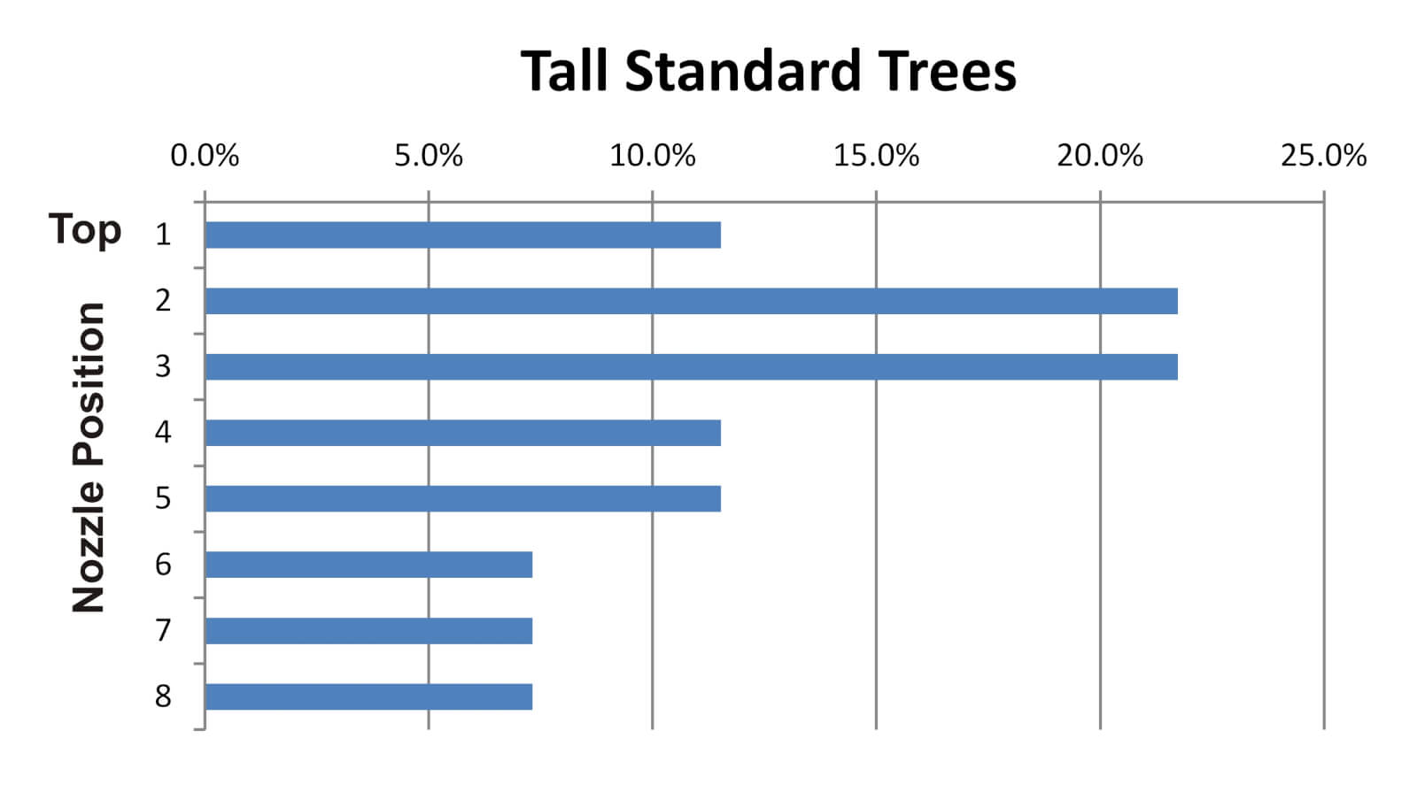
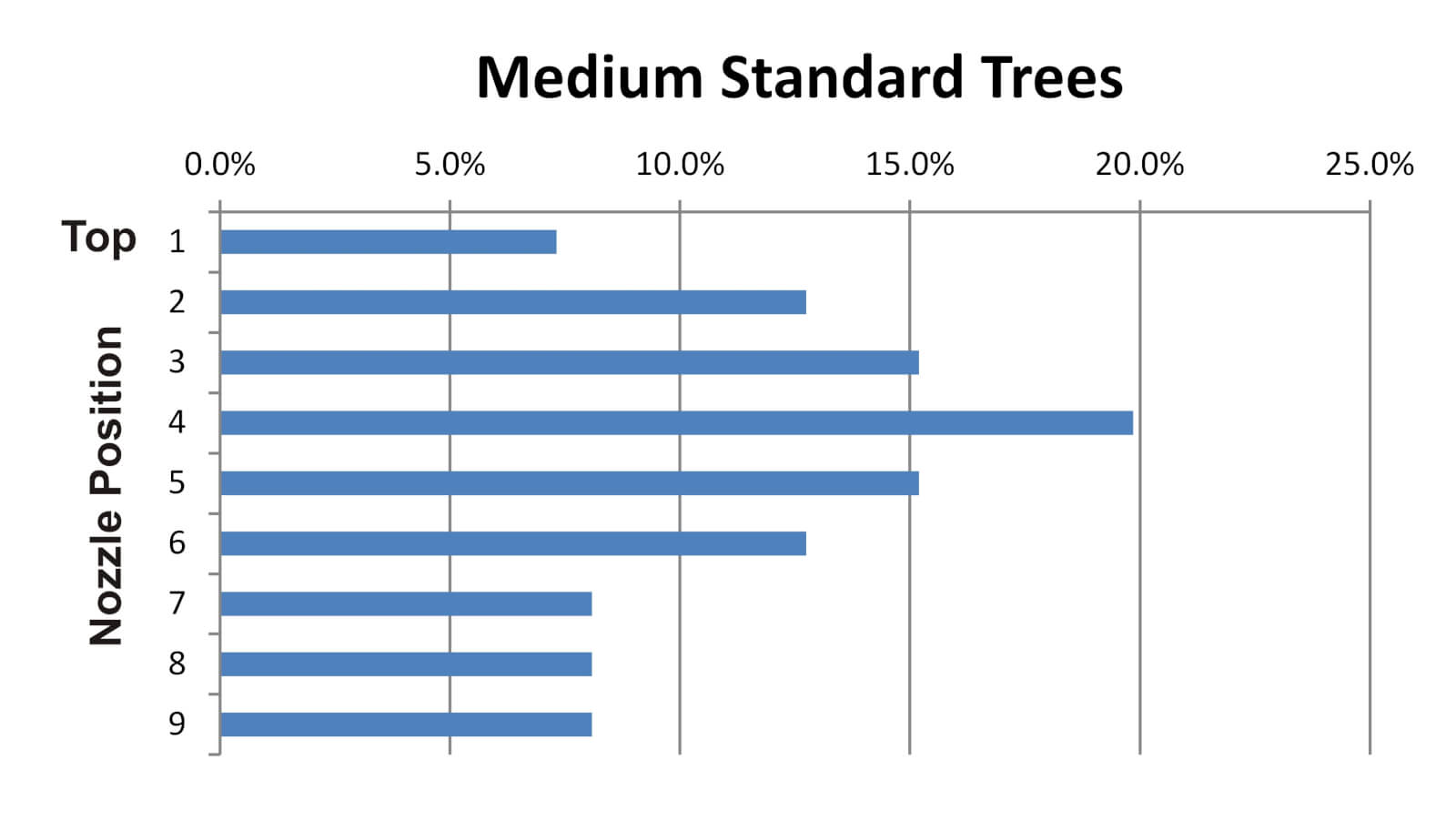
It seemed operators were getting away from high rates in the top positions and instead shifting the distribution to match the canopy shape and density. If we were to follow these recommendations, the spray profile would look something like this:
This begins to resemble advise found in Agriculture Canada’s 1977 publication entitled “Air-Blast Orchard Sprayers – A Operation and Maintenance Manual“. Here we find the “2/3 boom rule” as the authors state: “To ensure good distribution through the trees, about two-thirds of the spray should be emitted from the upper half of the manifold.”
1980s
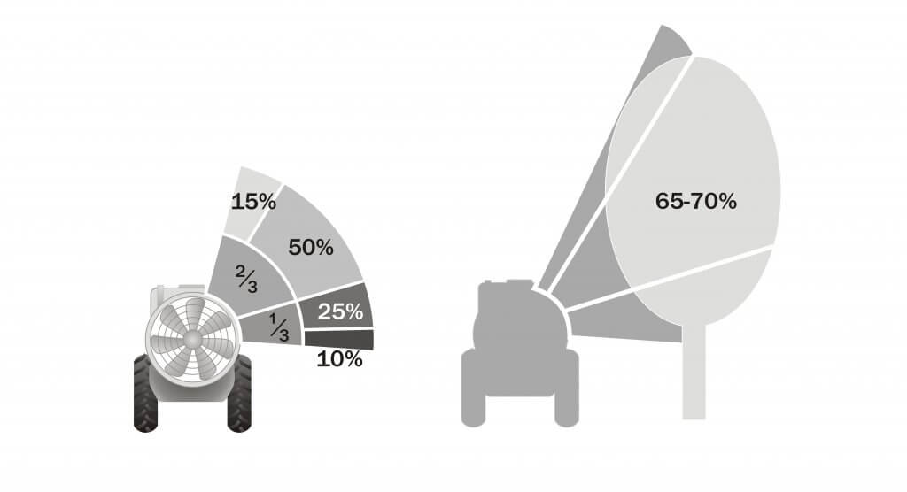
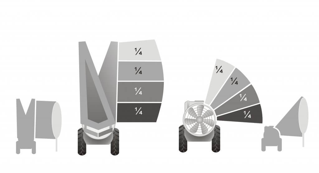
Operators followed this approach well into the 80s, as they endeavored to aim the majority of the spray into the densest part of the canopy. Many can relate to the following illustration that divides the boom. The fractions represent the portion of the available boom. The percentages indicate the relative volume. Of course, it matters how large and how far away the target is for either the 2/3-boom or 70% rule to make sense (the middle volume zone is shown receiving 65-70% in the silhouette).
1990s-2000s
The 2/3 or 70% rules still work for standard nut and citrus trees, and perhaps for large cherry trees, but pome and tender fruit orchard architecture is densifying. In the 90s and 00s we started transitioning from semi-dwarf into trellised, high density orchards.
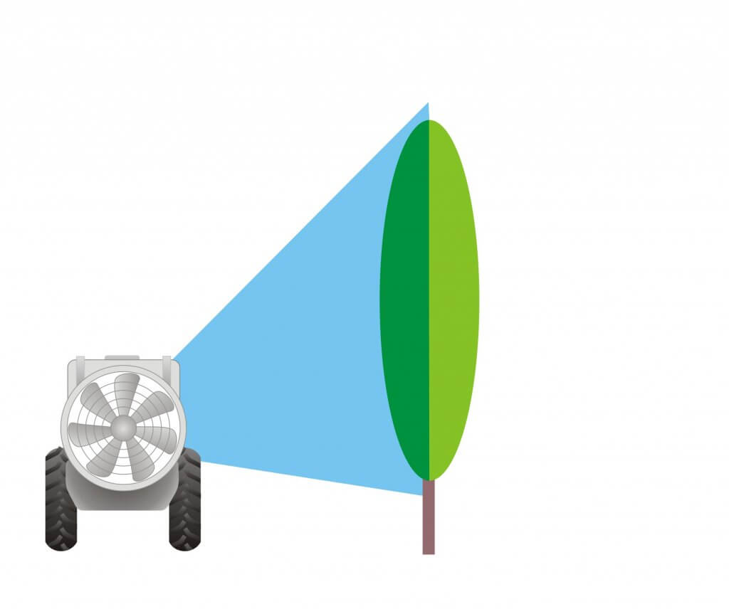
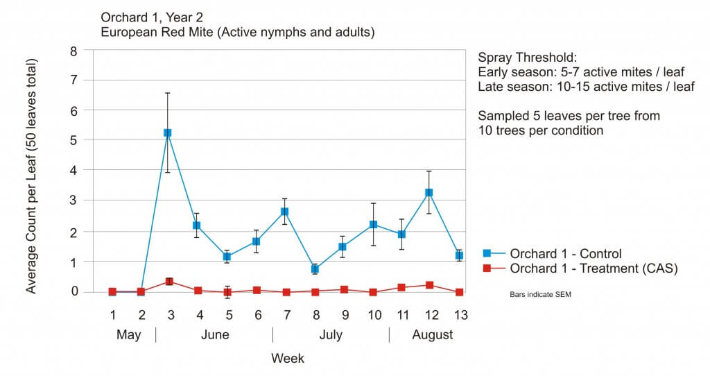
 In 2005, Ohio’s Dr. Heping Zhu et al., found that a high density orchard is effectively sprayed by the same rate in each nozzle position. They wrote: “[Historical] recommendations are to use a larger nozzle at the top of each side, with the capacity of the top nozzle at least three times greater than other individual nozzles. However, results in this study with three different spray techniques showed that spray deposit was uniform across the tree canopy from top to bottom with the equal capacity nozzles on the air blast sprayer.”
What a pleasant surprise to simplify our lives! If we can use an even distribution for dense, nearby trees, it follows that any vertical crop with the same width and density located close to the sprayer (e.g. cane fruit, trellised vines, etc.) would benefit from even distribution:
Today
So, how do we do it today? There is still no simple answer; Conditions change, not all sprayers are the same, and not all applications have the same target. Let’s build on what we’ve learned to establish a process to achieve better coverage uniformity and reduce waste.
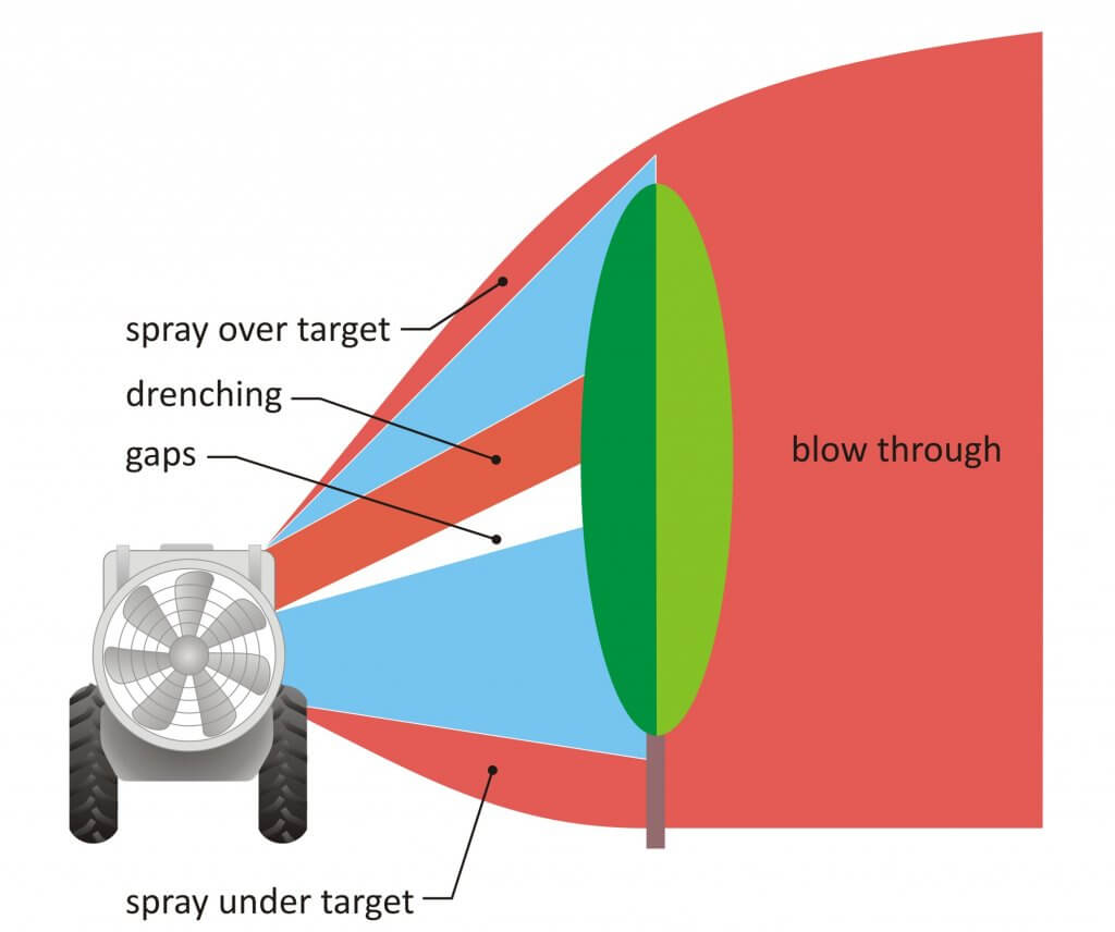
No matter the crop, the operator must first adjust air settings. Air volume and direction play the most critical role in transporting a droplet to (and into) a target canopy. Too high an air speed will cause spray to blow through the target, rather than allowing it to deposit within. Aim the air just over, and just under, the average canopy. Ensure there’s enough air to overcome ambient wind and to push the spray just past the middle of the target canopy.
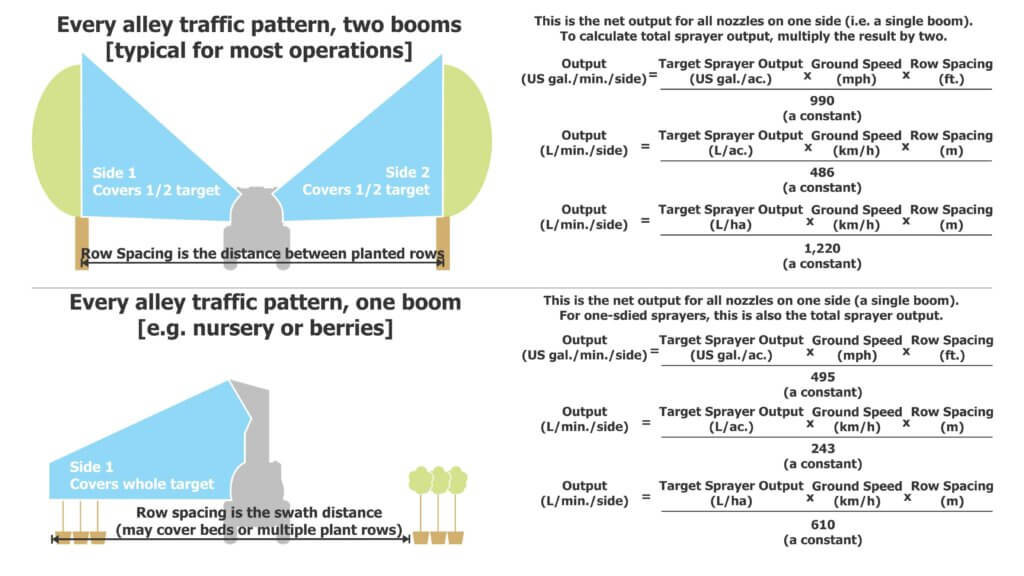
It should be noted that we assume the operator is spraying every row. With certain exceptions, alternate row middle spraying is not generally recommended. Not only can it compromise coverage on the far side of the target, it makes it far harder to match the nozzling on a single-row sprayer and is a sure-fire way to increase drift.
Next, determine which nozzles are not needed (e.g. spraying the ground or excessively higher than the top of the canopy). Remember: hollow cones overlap very close to the boom and spread as much as 80°. Airblast sprayers rarely if ever need the lowest positions and unless spraying overhead trellises they may not need the highest either. Turning off the highest, and most drift-prone, nozzle positions in high density orchards is illustrated very nicely in the logo of Washington’s 2017 Pound the Plume awareness campaign.
Then, finally, we decide on distribution. If the crop is nearby and relatively narrow, you can try even distribution. If you elect to distribute the spray unevenly to better match the variable-width target, or compensate for distance, aim half the overall output at the densest part of the canopy (the middle volume zone). Consider how the following factors might influence your choices:
High humidity means more spray will reach the target, and vice versa. This is because all droplets are prone to evaporation. We have heard it said in dry conditions a droplet can lose ½ its diameter every 10 feet. As they evaporate they get lighter, meaning they are less subject to their original vector and the pull of gravity, and more subject to deflection by wind. The use or coarser droplets, and/or humectants, can help, but higher volumes can help too – they increase the odds of some droplets hitting the target and actually humidify the air to slow evaporation.
Windspeed increases with elevation, so spray is most likely to deflect at the top of canopies where they have already lost size (and momentum and direction). Early in the season when there is little if any foliage, wind speeds are higher overall. This is why we advise adjusting air settings using a ribbon test before considering boom distribution – you need enough air volume, aimed correctly, to get the spray to the top.
The denser and deeper a canopy, the more spray is filtered and unavailable for coverage. This is why you will always achieve more coverage on the adjacent, outer portion of a canopy versus the interior. In semi dwarf apple orchards we have seen the coverage drop by half for every meter of canopy. Finer spray can penetrate more deeply because there are more droplets and they move erratically, whereas coarser droplets move in straight lines and impact on the first thing they encounter. Higher volumes will improve penetration and overall coverage, but there is a diminishing return and runoff will occur more quickly leading to more waste.
Further to the last point, remember that it’s the air that propels the spray, not the pressure. Higher liquid pressure can propel coarser droplets further, but has little effect on finer droplets. imagine throwing a golf ball and a ping pong ball into a light headwind and envision how they fly. Plus, the higher the pressure, the finer the mean droplet diameter.
Confirm Your Work
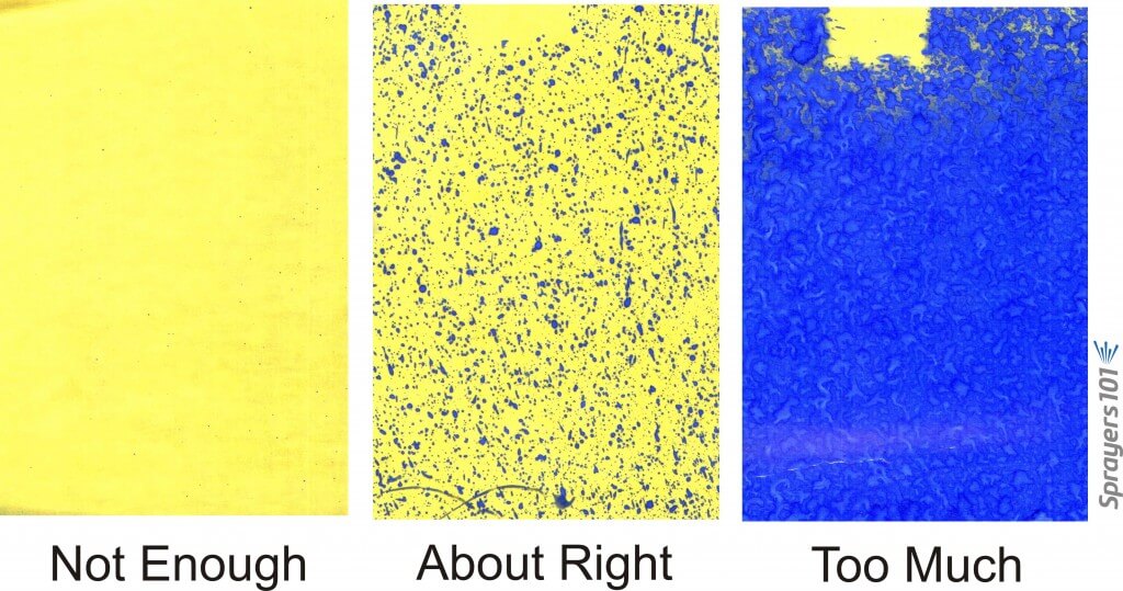
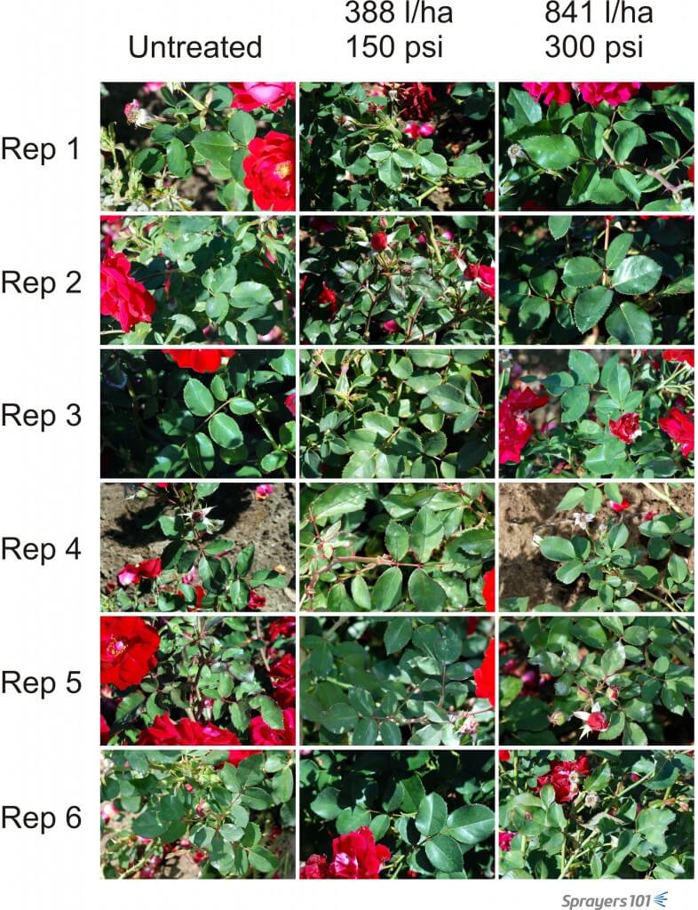
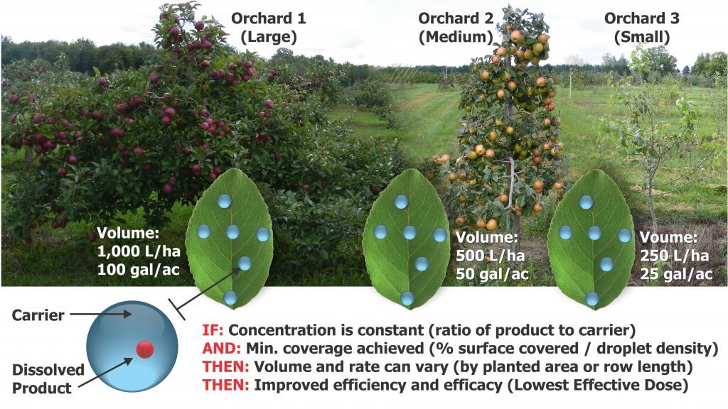
To know how all these factors play out, you must use water sensitive paper (or some other form of coverage indicator) to diagnose the results. Remember, the goal is uniform coverage and for most foliar products, we want to achieve a minimum coverage threshold of 15% and a droplet density of 85 deposits per cm2 on at least 80% of the targets.
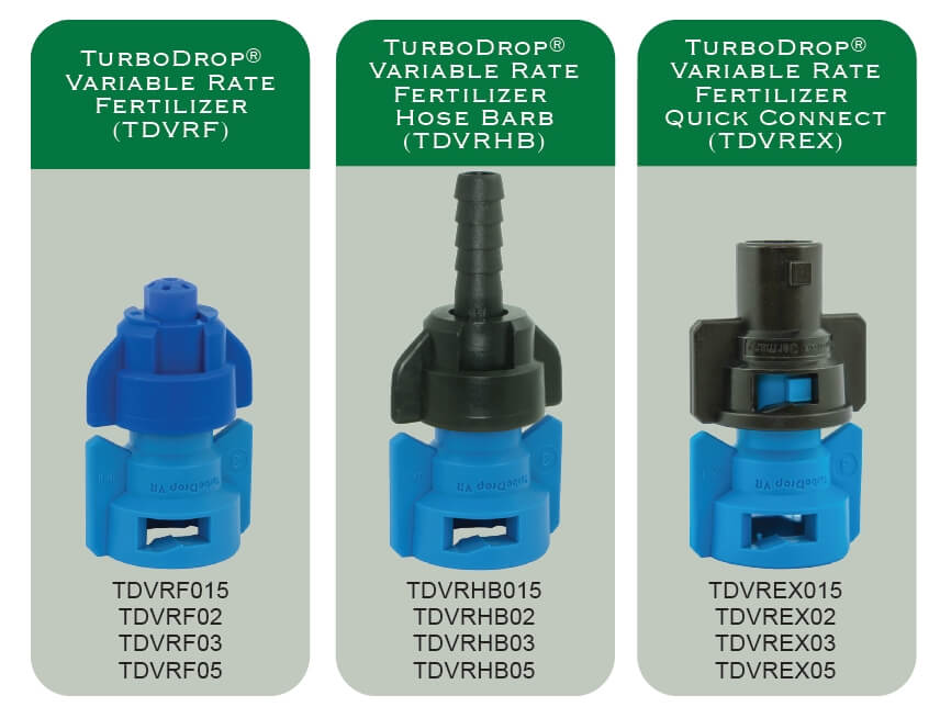
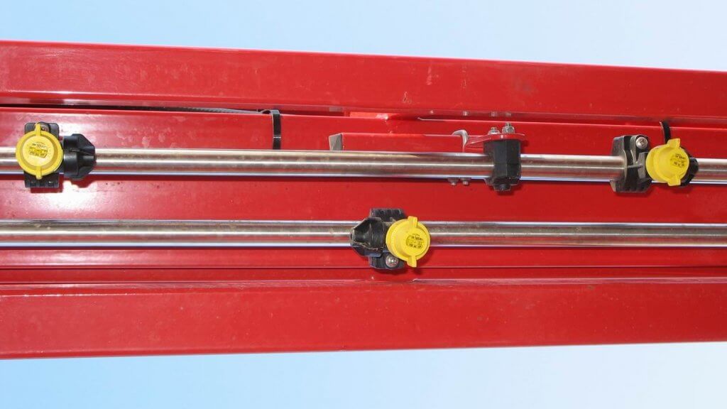
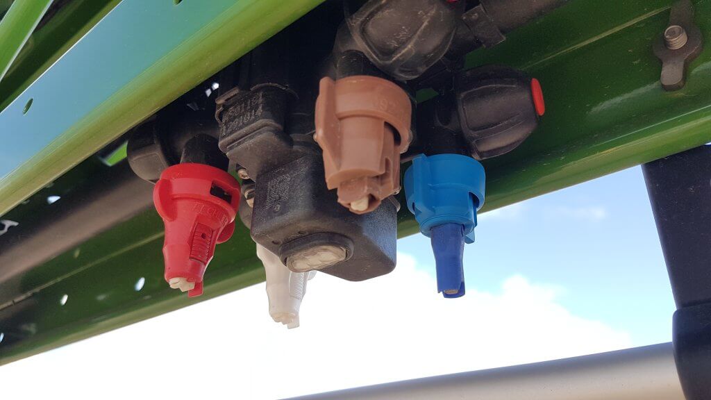
Taking the time to match your output to the target has the potential to greatly improve coverage and reduce waste. Nozzle body flips and quick-change nozzle caps make the process of switching nozzles between blocks fast and easy. It’s worth it.
Grateful thanks to Mark Ledebuhr, Gail Amos and Heping Zhu who edited, corrected and contributed to this article.
We always admire the photos of sprayers in tulips produced by the Netherlands. Rose protection in Ontario is equally beautiful.
Nursery growers apply pesticides to a diverse range of plant species. In a perfect world, sprayer operators would adjust their sprayer set-up to match each crop, but this is rarely done because of time constraints and a lack of guidance. Adjustments in product rate and spray distribution should reflect the plant size, row spacing and developmental stage of the crop and pest. Any such adjustments should be performed using a reference point for coverage and a strong history of efficacy.
To demonstrate the value of sprayer optimization, we marked out three, 65m x 6.5m blocks in a field of roses. One block was an untreated control. One block was the grower’s traditional set up of hollow cones (D4D45) on 50 cm centres at 300 psi and 3.0 mph (841 L/ha). The third block was the experimental condition where we used an optimized set up of hollow cones (D3D45) on 50 cm centres at 150 psi and 3.0 mph (388 L/ha). We validated this condition using an iterative process to dial in the coverage indicated by water-sensitive paper.
Setting up water-sensitive papers in the rose blocks.Rule-of-thumb fungicide coverage on water-sensitive paper.
One application of Folpet + Nova was made on Sep 19, 2011. Roses were photographed before and after the treatment. The photographs were digitized and the amount of powdery mildew appearing on the upper surfaces was determined as a percent of the total visible leaf area. Six replications were randomly selected from each block.
Visual record of randomly selected roses prior to treatment (September 9).Visual record of randomly selected roses immediately following treatment (September 20).
There was no significant difference in the amount of mildew presented in the two sprayed blocks one day after the application (September 20). Eight days after application (September 27), there appeared to be better control in the optimized sprayer set up condition versus the grower’s standard set up. The large standard error bars in the grower’s condition made this statistically insignificant. It is unclear why the untreated block presented with the least visual mildew at this point. This preliminary work demonstrates the value of customized application settings and their potential to conserve pesticide, water, and fuel without compromising pesticide efficacy.
Results of optimizing sprayer set up on the visual occurrence of powdery mildew on rose leaves. Bars represent standard error of the mean. Unclear why control block presented less mildew on Sept 27.
The Ontario Farm Innovation Program and the grower co-operator are gratefully acknowledged for making this research possible.
Variable rate spray application is receiving a lot or attention with our increased ability to farm according to prescription maps. For dry products such as seed or fertilizer, metering is relatively straight-forward and variable rate application has been possible for many years. However, liquid product application has been more complex and requires special approaches
Hydraulic Pressure and Flow Rate
In conventional liquid metering, the liquid is forced through a metering orifice that is placed in-line. This could be an orifice plate for liquid fertilizer, or a flat fan nozzle for pesticides. Rate control is achieved by altering the spray pressure. It is usually impractical to change the nozzle or metering orifice during an application.
The main drawback to this approach is that spray pressure is not very effective at changing flow rates due to the square root relationship between spray pressure and flow rate.
For example, with reference to the table below, one can see that doubling the spray pressure (say, from 30 to 60 psi) only increases the flow rate by 40%. Tripling the pressure (from 30 to 90 psi) increases the application volume by 73% (we can call that a factor of 1.73). As a result, the use of pressure alone doesn’t offer a large range of application rates, and we accept a factor of 2 to be the limit for fertilizer streamer and broadcast nozzles (meaning a four-fold pressure range) and a factor of 1.73 to be practical for broadcast pesticide sprays over a 3-fold pressure range. Any wider application volume range would require adjustment to travel speed.
With these inherent limitations in flow rate capacities from hydraulic pressure alone, applicators are often forced to use wide pressure fluctuations to achieve reasonable rate responses. In some cases, this means that pressure needs can be too low for uniform distribution, or too high for pump or plumbing capacities.
For Variable Rate application, we are less interested in travel speed range, and are more interested in flow rate range. The above chart can be used for both purposes. In the above example, rows under each application volume identify the travel speed range. These headings can be flipped, so the 10 gpa column (with mph values in it) can also be a 10 mph column (with gpa in it). the numbers don’t change. same is true for metric units, except the convenience of being in the same magnitude that makes the flip easy in US units is absent.
There are a few options available that expand the flow rate range of liquid products. A brief overview of the main options follows:
Greenleaf / Agrotop
TurboDrop Variable Rate (TDVR): This nozzle appears like the traditional TurboDrop family, but has an innovative dual orifice in its venturi. The first stage is always open, but the second orifice is held closed under spring pressure until a certain threshold is reached. This design achieves a 3-fold flow rate range between 40 and 140 psi. Below the 40 psi threshold, the spray pattern fan angle deteriorates quickly.
TurboDrop VR tip provides about 3-fold flow rate range at any given speed, but requires higher pressures.
TurboDrop Variable Rate Fertilizer (TDVFR): Because fertilizer streams do not need to atomize the spray or form a fan, the minimum pressure can be reduced, in this case to 10 psi. From 10 to 140 psi, this design offers a four- to five-fold range of flow rates. Three exits are offered, a streamer, a hose barb, and a quick connect.
Three variants of the variable rate fertilizer orifice are offered by Greenleaf.
VariTarget Nozzle
This nozzle design uses a spring-loaded plunger to exert force on a flexible nozzle cap, deflecting it slightly. The deflection changes the orifice size, allowing for a change in flow. As a result, the flow rate response to a pressure change is increased dramatically. A single VariTarget nozzle equipped with a blue or green nozzle cap can deliver flows ranging from 0.2 US gpm at 20 psi to 1.2 gpm at 65 psi, for a stunning 6-fold change in application rate (link).
The VariTarget nozzle body
The main drawback of this nozzle is the poor metering accuracy of the system. In calibration tests, flows from various new VariTarget nozzles operated at the same pressures varied by more than 10%. While this amount of variability may be acceptable in liquid fertilizer application, it is not considered acceptable for pesticide application. Tightening or loosening the threaded spring cap even a little changes the flow.
TeeJet Variable Rate Fertilizer Assemblies
These metering assemblies, introduced in 2016, offer an elastomer (EPDM) metering plate whose orifice diameter expands with pressure, offering a wider range of flows. There are no moving parts in the assembly. Four models are available (link).
PTC-VR: Using a push-to-connect design for planters and toolbars, it offers versions that accomodate 1/4″, 5/16”, and 3/8” OD tubing diameters
QJ-VR Hose Barb: This unit offers hose barb diameters for 1/4″ and 3/8” ID hose.
Both units feature a pressure range of 10 psi to 100 psi, within which a flow rate range of approximately 8-fold is possible.
SJ3-VR: This unit generates three streams and operates over a pressure range of 20 to 100 psi, offering a flow rate range of about 3-fold.
GPA ranges for specific travel speeds for TeeJet SJ3 VR
SJ7-VR: Generating seven streams and operating over a pressure range of 30 to 80 psi, this unit allows a flow rate range of about 2.9.
In all cases, the realized flow rate range is significantly greater than would have been achieved with pressure change alone. TeeJet has tested the flow rate variance among units operating at the same pressure and has found them to be acceptable, according to company representatives.
Fertilizer banding has greater tolerances for application because pattern width is less important, and also because stream stability is less affected by pressure than spray pattern droplet size.
Pulse Width Modulation (PWM)
PWM utilizes conventional plumbing: a single boom line and a single nozzle at each location. Liquid flow rate through each nozzle is managed via an intermittent, brief shutoff of the nozzle flow activated by an electric solenoid that replaces the spring-loaded check valve. Typical systems pulse at 10 or 15 Hz (the solenoid shuts off the nozzle 10 or 15 times per second), and the duration of the nozzle in the “on” position is called the duty cycle (DC) or pulse width.
100% DC means the nozzle is fully on, and 20% DC means the solenoid is open only 20% of the time, resulting in the nozzle flowing at approximately 20% of its capacity. This is illustrated in the figure below. The ability to control the duty cycle is referred to as pulse width modulation.
The system has a theoretical flow rate range of about four- to five-fold. Within this range, spray pressure, and the corresponding spray pattern and droplet size, stay roughly constant. This makes it ideal for variable rate pesticide application, where spray patterns and spray quality are critical for performance.
The main disadvantage of this system, compared to the variable orifice designs, is cost. Although highly accurate and dependable, commercial sprayer units are priced between $15,000 and $65,000 per sprayer, depending on features and boom widths. The available systems are Capstan PinPoint II and EVO (as a retrofit to any sprayer), Raven Hawkeye (retrofit to any sprayer, available as factory option on Case (AIM Command), New Holland (IntelliSpray) and most other brands, John Deere ExactApply, WEEDit Quadro, Agrifac StrictSprayPlus and TeeJet DynaJet (available as retrofit). See our in-depth article on PWM for more information on these systems.
For ammonia and liquid fertilizer planters or toolbars, Capstan offers three different PWM products, N-Ject NH3, N-Ject LF or EVO LF. These systems offer more control over PWM pulse frequency and duty cycle and can achieve 8-fold rate ranges.
Flow rate ranges for Capstan N-Ject LF, on 30″ spacing
At low frequencies and duty cycles, the mobiliy of the fertilizer in soil needs to be considered, as significant gaps in a stream can be generated.
A variable rate for liquid fertilizer system for seeders, together with sectional control and turn compensation, is offered by Capstan EVO-LF. This system can generate 10 to 60 gpa at 4.5 mph on 12″ spacing.
Dual Boom Systems
A second boom fitted with different flow nozzles is installed, and is activated when the flow rate requirements can no longer be met with a single set of nozzles. Once the second boom is activated, the spray pressure drops significantly and additional flow capacity can be realized.
Dual boom system
Dual or Quadruple Nozzle Bodies
A similar approach to the dual boom is available as selectable nozzles in the same body from Arag (Seletron), Hypro (Duo React), John Deere (ExactApply) Amazone (AmaSelect), and others. These systems utilize a single boom and direct the flow through one of any two (Duo React, ExactApply, Seletron) or four (Seletron, others) nozzles, or several nozzles at the same time.
AmaSelect utilizes a unique switching system that allows the user to select only Nozzle 4, Nozzle 3, Nozzles 3 & 4, and Nozzles 2 & 4, making the placement of certain sized nozzles critical.
Amazone AmaSelect nozzle switching system
Similar pressure fluctuations as with a dual boom would be experienced, requiring careful selection of nozzle flow rates to avoid large pressure jumps. The system can also be used to manually change from one nozzle to another as needed. In the figure below, the pressure changes associated with the sequential use of 015, 02, and 035 flows are shown.
Direct Injection
Direct injection is an option for variable application of pesticides. In this system, undiluted pesticide is placed into canisters on the sprayer, and plain water (or water plus adjuvant) is in the sprayer tank. The chemical is metered and introduced into the water on the pressure side at some distance upstream from the boom sections. The pesticide rate can be varied with the speed of the direct injection pump, offering a very high dynamic range of possible rates. For example, Raven’s Sidekick Pro (available as factory option on Case and John Deere sprayers, or as a retrofit to any sprayer) offers a 40-fold range of flow rates.
After injection, an in-line mixer ensures that products are evenly distributed in the carrier. The amount of lag in the systems will depend on the amount of spray mixture in the plumbing upstream of the nozzles, the total boom flow rate, as well as the boom section configuration. With a variable rate map this lag can can be anticipated and accommodated.
Pump technology has improved the metering accuracy over a range of viscosities. However, dry formulations remain a challenge as slurries can settle and create problems for the pump and screen components.
Summary
High dynamic flow rate ranges for agricultural sprays are challenging to achieve, but will become more important as interest in site-specific management increases. Relatively inexpensive solutions are available for liquid fertilizer, whereas pesticide sprays require greater investments in technology to preserve spray pattern integrity. As mapping sophistication continues to grow, these application technologies will be integral to variable input prescriptions.
Here’s a common situation: An orchardist following IPM identifies a pest that poses an economic threat. It’s an annual pest and spraying is really a matter of when, not if. The operation is 150 acres and runs three airblast sprayers; two have a tower and one does not. Multiple varieties are planted in several blocks on different rootstocks and they are at different stages of maturity. The newer blocks are trellised high density trees and the older blocks are semi-dwarfs on different row spacing. Let’s also imagine the pruning team hasn’t finished yet, so some trees are not pruned.
The orchardist turns to the pesticide label to decide how to spray such variable targets. It prescribes a range of doses per planted area (not canopy size), depending on the pest pressure. It advises the orchardist to use “enough water” to ensure “good coverage” without incurring “runoff”.
The orchardist recognizes that the label is vague, and elects to rely on what has worked historically: A water-soluble pouch is dropped into each tank (dose is close enough), and each sprayer operator is instructed to drive at an efficient speed (get it done because rain is coming), spraying until the tank is empty. They say that if a tank is running low before the job is done, speed up and stretch it. If the spray is overshooting a younger planting, they suggest turning off the top nozzles and/or driving faster.
Airblast operators face this situation regularly. The question is: “Is there a problem with spraying this way if it results in a respectable crop of quality fruit?” Agricultural engineers specializing in application technology in Spain, Australia, Great Britain and the United States say there is a problem, and on behalf of Canada, I completely agree with them.
Canopy and Sprayer Variability
The fundamental problem is inconsistent spray coverage and avoidable waste (of time, water and pesticide) due to variability. Our scenario notes multiple sprayer operators, different models of sprayer, and a range of varieties, orchard architectures and canopy management practices. The label does not allow for any of these factors, adhering to a rate based on planted area and remaining silent on water volume.
International peer-reviewed journal articles stretching back to the sixties have conclusively demonstrated order-of-magnitude differences in the area-density of orchard canopies from one acre to the next. There can even be fold-differences in canopy area-density in the same planting as the season progresses. A label prescribing a fixed dose based on the area planted is not appropriate for any vine, bush, cane or tree crop, and the result is that more crops are over- or under-sprayed than receive appropriate coverage.
Let us not forget the variability that comes from a poorly adjusted sprayer. I won’t to attempt to quantify the impact (although some researchers have suggested order-of-magnitude differences from sprayer to sprayer). Instead, let’s illustrate it as a conceptual “before and after”:
Before: Potential spray loss and inconsistency before adjusting sprayer to match the canopyAfter: Coverage variability reduced and unnecessary waste mostly eliminated.
Beyond the immediate impact on efficiency, variability makes it difficult to diagnose pesticide effectiveness. As an example, there was a scab outbreak in Ontario in 2009 that elicited questions about timing, weather, product choice and resistance. There was very little attention given to spray coverage, which to my mind should have been the first question if only to eliminate it as a potential culprit. This is because each operation interprets labels differently, and very few confirm coverage in any quantifiable way. This practice makes it more difficult to identify a cause when crop protection fails.
Optimizing pesticide rates
That was a lot of preamble to describe an issue that many orchardists are already aware of. What is needed is a way to adjust the amount of pesticide per unit ground area (i.e. the label’s prescription) to achieve consistent foliar coverage for canopies of varying shape and density. The concept is visualized in the following figure. In addition, the method has to be simple, intuitive and effective.
Many models have been proposed to tackle the dose expression issue, including Tree-Row Volume, Leaf Area Index, Leaf Wall Area, PACE+ and DOSAVIÑA. There are advantages and disadvantages to each method. Standing on the shoulders of giants, we combined aspects of each of these models, including incorporating coverage factor research from USDA ARS work in nurseries, to develop the Crop-Adapted Spraying (CAS) method. It is neither complicated nor sophisticated. It formalizes a series of qualitative calibration techniques and the objective is to achieve a target foliar coverage pattern. When achieved with sufficient accuracy, pesticide efficacy is maintained and waste is greatly reduced.
Caveats
Perhaps I shouldn’t point out flaws before I describe the model’s effectiveness, but it’s important to understand that CAS relies on a few critical assumptions.
The first assumption is that the sprayer operator’s typical ratio of formulated product to carrier is appropriate. We need a starting point for adjusting the amount of pesticide per unit planted area, and unless the label specifies a concentration (i.e. a ratio of formulated product to water) or a minimum amount of product per planted area, this is a reasonable starting point. The appropriateness of this assumption is evidenced by a history of satisfactory pest control in the orchard.
The second assumption lies in defining a threshold for sufficient coverage, and this is a real challenge. Applications can be concentrate or dilute. Some products translocate in the leaf or redistribute on the leaf surface while others do not. Even the droplet size employed (e.g. A mist blower’s fines compared to Medium-Coarse droplets produced by an air induction nozzle) will affect dose, bioavailability and how long residues are active. So, how does one draw a universal line in the sand and say “this much is enough”?
Our threshold for suitable foliar coverage has evolved through experience, literature review and independent experimentation in several countries and in multiple 3D cropping systems. We propose 10-15 % surface coverage and a minimum of 85 droplets per cm2on a minimum 80% of the canopy. This standard is intended to be practical, versatile and robust in order to safely represent sufficient coverage for most foliar insecticides and fungicides. It is not suitable for ultra-low volume sprayers (e.g. misters, foggers, air-shear), nor is it intended to be a rigorous, scientific absolute.
For example, a drench application, such as streptomycin or dormant oils, will obviously require more coverage. Plant growth regulators like thinners, stop-drops and foliar nutrients have their own unique criteria. Products that work through vapour redistribution (e.g. some forms of sulfur) and bio-rational products have a minimal dose threshold that must be ensured per planted area, no matter the water volume used. In these cases, Crop-Adapted Spraying may not be appropriate.
So while it is the nature of models that they may not hold in every situation, this threshold has proved successful in multiple Ontario apple (later in this article) and highbush blueberry operations.
The method
The method is a simple and iterative approach that allows growers to adjust the product rate and sprayer output in relation to canopy and sprayer effects on deposits. Follow these steps to adjust the sprayer and optimize coverage. Only do so in conditions you would normally spray in.
Step 1
The sprayer should receive all seasonal maintenance prior to first use and undergo a visual inspection before each spray day.
Step 2
Park the sprayer in an alley between rows of trees and tie 25 cm (10 in) lengths of ribbon along the air outlet. That would be the deflectors on a low profile axial sprayer, the hubs of multifan systems or the ducted outlets on towers. Turn on the air and extrapolate where the air is aimed. Adjust the air to just overshoot the top of the canopy.
Step 3
It is important that the spray slightly overshoot the canopy height. It is less important to spray the lowest point of the canopy as secondary deposition tends to provide sufficient coverage. This may change if fruit weighs down the branches. Ensuring a full swath, turn off any nozzles that are not required. For small and medium canopy sizes, consider using air-induction hollow cones in the top positions of each boom to reduce drift. You may have to increase the rate in those positions to compensate for the fact that nozzles producing larger droplets produce fewer droplets.
Step 4
Affix 25 cm (10 in) ribbons to the upwind and far side of one or more trees. At minimum, affix them at the treetop and along the widest portion of the canopy. With the tank half-full of water, drive past in the spraying gear at the ideal RPMs with the air on. A partner in the next alley should see the highest ribbon move. Ideally the other ribbons will waft as well, but in large, dense canopies they may not. In this case, ensure leaves are moving beyond the trunk. No ribbons should strain straight-out.
This will determine if more/less air is required from the airblast sprayer. The operator can change fan speed (e.g. fan gear), or adjust the sprayer’s travel speed. Lower speed causes air to go higher and deeper and vice versa. In some cases, operators can reduce fan speed by reducing the tractor PTO revolutions by gearing up and throttling down. When air is corrected, determine ground speed in the orchard using smartphone GPS app or a calibration formula.
Step 5
Place and interpret water-sensitive papers per this article. If coverage is excessive, reduce output in corresponding nozzle positions (by replacing them with lower rate nozzles). If you see less than ideal coverage, increase the nozzle rates in those positions.
Be aware that excessive coverage may be unavoidable in the outer edge of the canopy, given that spray must pass through to get to the centre. It is not unusual to see half the deposition mid-canopy when the outside is saturated. Also be aware that ambient wind speed and humidity have significant impacts on coverage. Therefore, only test coverage in conditions similar to your typical spraying conditions.
Step 6
When the canopy grows and fills in sufficiently (usually after petal fall), you may have to reassess coverage to reflect a larger, denser canopy with more surface area. Given the critical nature of early season fungicide applications, it may be preferable to have slightly excessive coverage early season and allowing it to self-correct as the season proceeds. If you are suspicious that the spray is being stretched too thin or you are unsatisfied with the coverage, increase the output.
For high density trees, there may be no need to increase output mid-season. Early in the season, wind travels relatively unimpeded in a high-density orchard and will blow spray off course, reducing coverage and requiring higher water volumes or possibly more air to compensate. As the trees fill in, the average wind speed is reduced and more spray can impact on the target.
Mixing and Work Rate
When the correct sprayer settings and volumes have been determined, the operator will mix their spray tank as they would for their typical application. The sprayer will likely cover more orchard than it has in the past, and the operator will have to re-assess how many tanks are required pre and post petal-fall. If your sprayer is employs conventional hydraulic nozzles (that is, it is not a low-volume sprayer), it is not advisable to go below 400 L/ha (~40 gpa).
This is where OrchardMAX (the free CAS calculator app) can help the operator ballpark the correct rates for each nozzle position and estimate work rate, tanks required, and any potential savings in product.
Yes. There’s an app for that.
Apple Orchard Case Study
Three Ontario apple orchards (and one Nova Scotia orchard) agreed to test the model. A block of trees was randomly selected from each operation to serve as the treatment condition. These trees received spray according to the CAS model. The rest of the orchard was sprayed according to the grower’s traditional methods. The orchards included several varieties and represented both semi-dwarf and high density plantings.
Orchard
Typical spray volume (Control)
CAS spray volume (Treatment)
% Savings
Varieties (age)
Orchard Structure
Years in study
Orchard 1
486 L/ha
373 L/ha
23%
Gala + g. Del (~10 yr old)
High density
3
Orchard 2
748 L/ha
478 L/ha &
608 L/ha = 543 L/ha
28%
Macs + Empires (~30 yr old)
Semi-dwarf
3+
Orchard 3
577 L/ha
(660 L/ha)
407 L/ha
39%
(38%)
Gala + Fuji (~20 yr old)
High density
2
Nova Scotia
544 L/ha
416 L/ha
33%
Jonogold (~10 yr old)
High density
1+
According to the model, each grower sprayed anywhere from 20-35% less per hectare in the CAS block than in their traditionally-sprayed block. In many cases, the overall canopy coverage was improved in the CAS block compared to the traditional method simply by aiming formally wasted spray into the canopy, and reducing volume in those areas that were unnecessarily drenched.
A scout was dispatched to monitor insect and disease activity each week for ~15 weeks. They observed a typical IPM scouting protocol and were not informed which block was the traditional control and which was CAS treatment. Data was transformed where appropriate for analysis of variance. In almost every case, there was no significant difference in counts between the CAS treatment and the grower’s traditionally-sprayed control (p=0.05). In those few cases where a pest had higher counts in the CAS block, the counts were so far below a spray threshold as to be insignificant.
If we look more closely at the three (of 128) ANOVA comparisons of control to treatment, we see that economic thresholds are rarely an issue, and essentially, difference between control and treatment are moot.
This study was repeated over three years. Having examined the data to determine if three years of optimized doses had any effect on pest populations, results suggest no such effect.
Apples were randomly sampled for destructive analysis at harvest and the total counts of any and all damage are shown below. This is simply a tally, and no statistical significance is implied. Note that Orchard 3 was only involved in the study for two years, and unfortunately a killing frost destroyed their harvest in their second year, so we didn’t have much to harvest.
An important part of knowledge transfer is whether or not growers will choose to adopt a method once the instructor is gone. By year two the biggest challenge was ensuring the orchardists in the study continued to spray the control block at their traditional volumes! They were more than willing to adopt the method wholesale and all three did so starting in 2016. Further, colleagues in Nova Scotia performed their own CAS trial for two years, and reported no significant difference in pest activity or apple quality. They accomplished this simply by following a written protocol.
The orchardist’s enthusiasm, the ability for the study to be replicated without my direct involvement, and the successful results speak to the viability of the method.
We would like to thank the researchers that developed the methods CAS is based upon, statistician Behrouz Eshani, the orchards that cooperated in the study, my OMAFRA colleagues and the OMAFRA summer students that scouted those orchards for three years.
More information
This method of application is really no more sophisticated than the pro rata practice of turning off nozzles that are aiming at the ground or above the target. It will take time for operators to get comfortable with the new volumes (and potentially reduced dosage) and regular scouting is highly encouraged to confirm they are achieving control.
The maintenance, calibration and operation of an airblast sprayer is an involved process. Collectively, the sprayer setup, weather and crop morphology all influence the coverage obtained from an application. A fundamental understanding of application technology is required before attempting to optimize dosage using the CAS method. We suggest grabbing a copy of the second edition of Airblast101 – Your Guide to Effective and Efficient Spraying. The digital version is a free download, but you can buy a hardcopy as well.
Finally, take a few minutes to watch this video by AAMS-Salvarani. In many European countries such as Belgium , France and Germany, sprayers must be calibrated regularly. While there is no mention of air speed adjustments, many of the steps in this video correspond with the airblast adjustments relating to Crop-Adapted Spraying.