When T3 wheat rears its head, the first rainy day brings questions about spray angles. Let’s begin with a graphic that illustrates how angled sprays cover a vertical target like a wheat head. Assuming moderate wind and sufficiently large droplets, this is a simplified depiction of what we would expect to see.
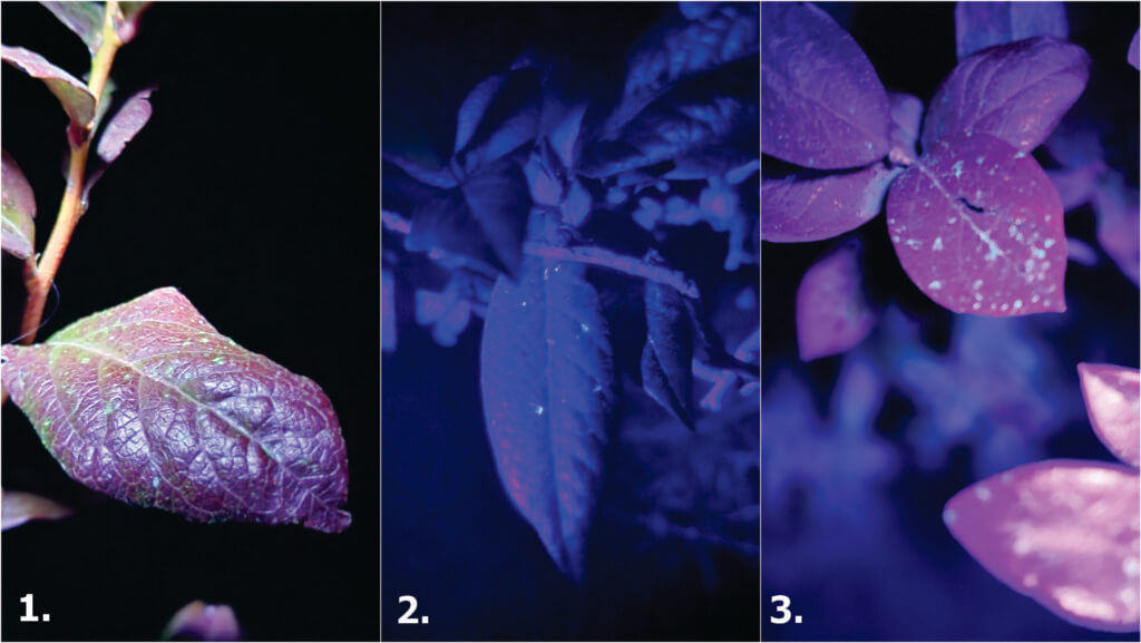
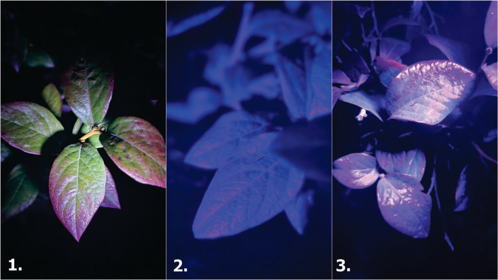
But is this how the nozzles actually perform? Are dual angles really better than a single fan with an aggressive angle? We hoped to answer these questions when we demonstrated a selection of dual fan nozzles at Canada’s Outdoor Farm Show in 2013. But it was a very windy few days and what we saw was that regardless of the nozzle, most of the spray tended to deposit with the wind.
A 10 km/h wind will easily deflect Medium-and-smaller droplets and at 20 km/h all but the coarsest spray is deflected. This leads to non-uniform deposits and unacceptable levels of drift (yes, even through it’s a fungicide and you have lots of acreage.) To learn more, we turned to the literature to review studies performed in Ontario and Saskatchewan.
Wolf and Caldwell
In 2002, Dr. Tom Wolf and Brian Caldwell experimented with fan angles. They evaluated the impact of nozzle angle, travel speed, and droplet size on the “front” (facing the sprayer’s advance) and “back” (sprayer’s retreat) of vertical targets. They ran three laboratory experiments: spray configuration (single vs. double fan), travel speed (7.6 and 15.2 km/h) and spray quality (conventional versus air-induced droplets) using TeeJet XR’s and Billericay air bubbles at a rate of 175 L/ha. Here’s what they observed:
- Larger, air-induced droplets produced higher average deposits than smaller, conventional droplets.
- Twin fans improved overall average deposit compared to single fans.
- Building on the first two points, twin air-induction fans improved overall average deposit versus conventional twin fans, and also improved deposit uniformity (i.e. coverage on the front versus the back of the vertical targets).
- Higher travel speeds improved overall average deposit, but at the cost of reduced uniformity as the rear-facing target received reduced coverage (particularly in the case of conventional droplets).
- Spray angle did not impact coverage from conventional tips, but increasing from 30 to 60 degrees improved coverage for AI tips.
While the coverage data was compelling, growers were not reporting improved efficacy with the improved coverage. The authors felt there were confounding variables like crop susceptibility, disease pressure and product effectiveness. Their conclusion was that applicators should strive for improved coverage, but only after integrated pest management (IPM) criteria such as product choice, crop staging and application timing are satisfied.
Hooker and Spieser
In 2004, Dr. David Hooker (University of Guelph) and Helmut Spieser (OMAFRA) started exploring nozzle configuration and sprayer set-ups to optimize Folicur applications in wheat. For several years they ran field trials exploring panoramic wheat head coverage. That is, not only the front and back of the wheat head, but the sides as well. Ten different nozzle configurations were used:
- TurboTeeJets mounted in dual swivel bodies (backwards and forwards)
- AirMix air induction nozzles mounted in dual swivel bodies
- Air induced Turbo TeeJets mounted in dual swivel bodies
- Single Turbo TeeJets angled forward or angled backwards
- Single Turbo FloodJets angled forward or angled backwards
- TwinJets
- Single Hollow cones
- Turbo TeeJet’s mounted in Twincaps
- Turbo TeeJet Duos
- Single Turbo FloodJets alternating forward and backwards
They explored boom height (0.5 m and 0.8 m above the crop), travel speed (10 km/h and 20 km/h) and application volume (93.5 L/ha and 187 L/ha). Here is a summary of their findings:
- Travel speed did not appear to impact overall coverage.
- Spraying higher volumes improved coverage.
- Lowering the boom improved coverage.
- Coverage from conventional flat fans and TwinJets gave ~15-18% coverage and 22-26 mg of copper was deposited per m2, but alternating Turbo FloodJets gave ~29% coverage and deposited ~37 mg copper per m2.
- The highest percent coverage was obtained using Turbo TeeJets or the AirMix tips mounted in dual swivels (~26% coverage), or single Turbo Floodjets alternating forward and backwards (34% coverage) as long as the spray was not obstructed by the boom structure itself.
Hooker and Schaafsma
A few years later, Dr. Hooker and Dr. Art Schaafsma worked with OMAFRA to explore efficacy. DON is a mycotoxin that may be produced in wheat infected by Fusarium Head Blight (FHB) or scab. There is an indirect relationship between wheat head coverage of fungicide and the reduction of FHB and DON: The higher and more uniform the coverage (with the right timing) the lower FHB and DON.
In two field experiments they performed in 2008, DON values in the untreated checks were around four parts per million. DON was reduced by an average of 22.5% using a single flat fan, 23.0% using a TwinJet and 41.5% using alternating Turbo FloodJets when averaged across two fields, two fungicides and four reps (n=16). They all reduced DON significantly. There was no statistical difference between singles and twins, but control from the alternating Turbo FloodJets was significantly better.
The Return of Wolf and Caldwell
Then, in 2012, Tom and Brian evaluated the new asymmetrical twin fan nozzles from TeeJet. The marketing claimed they could improve overall coverage at higher travel speeds because they decrease the contribution of the front-facing fan and increased the angle of the back. Tom and Brian’s lab-based experiments determined that:
- Asymmetricals increased overall deposit amounts and uniformity versus single fan and symmetrical twin fans.
- Nozzle orientation (alternating or not) seemed unimportant.
- As suggested earlier, boom height was a big factor in coverage. Nozzle angle didn’t improve coverage when the boom was too high, but spray deposit increased significantly when the boom was lowered.
- Coarser spray droplets have more momentum, so they can travel greater distances on their original vector. A coarser spray quality is the best choice for any angled fan.
Water volumes and FHB
Let’s address the notion that high water volumes might increase Fusarium Head Blight (FHB). This is a hypothesis that seems to have resonated with growers. Dr. David Hooker ran trials where he tried to favour FHB by spraying 40-50 gpa of water multiple times per day (even up to 100 gpa). There was no pathological impact (personal communication).
Consider that 1″ of rain is the equivalent of 2,715 gpa of water. Raising your carrier volume from 15 gpa to 20 gpa is the equivalent of 0.000184″ of rain. Admittedly, it’s all aimed at the wheat head, but it’s still a tremendously small volume. While studies have shown a diminishing return in coverage at 30 or 40 gpa, spraying with 20 gpa appears to be a safe way to improve coverage significantly.
Learn more about early morning spraying here, and a more in depth discussion of spraying when there is dew here.
PWM
What if you’re running a PWM system? Sizing for PWM requires the tip be sized about 20-40% more than if you were running a conventional sprayer. In other words, at expected travel speeds, the pulsing duty cycle should be approximately 60-80%. Nozzles that are permitted on PWM sprayers are limited and the angled fan selection for PWM is, at the time of writing, more so. It requires some experimenting. The following list uses the JD Exact Apply as an example system, and it is not exhaustive. We’re always looking for new ideas.
- 3D90 (the original 3D is arguably too misty) in the A or B positions, alternating front and back <or> in both A and B positions. This tip may not be readily available in North America.
- LDT (Low Drift Twin) which is two LD tips installed in a Twincap (twin 30° angles) in position A or B.
- LDM (Low Drift Max) which is two LDM installed in a Twincap in position A or B. This tip only goes down to an 03.
- The Deere 40 degree angled adaptor (developed for See and Spray) can be used to convert any PWM-compatible nozzle into an angled spray.
- GAT (GuardianAir Twin) is an air-induced tip, running in conventional “A” mode or in Auto Mode but sized for “B”. Avoid operating in A and B to prevent pattern interference.
- Wilger Wye Adaptor with SR nozzles. This does cause tips to drop below the boom frame but is a versatile option.
- Wilger Dual Angle Max. More compact than the wye adaptor, this asymmetrical assembly (30° fore and 50° aft) prioritizes Coarse spray.
- TeeJet Accupulse TwinJet.
- Greenleaf Blended Pulse Dual Fan Assembly.
Summary
So here’s what we can say based on all this research:
- Higher volumes improve coverage (significantly up to ~200 L/ha or 20 gpa). Can you go to 30 gpa? Yes, and it will likely improve coverage, but it’s a diminishing return and at some point you will incur run-off.
- When using angled sprays, coarser droplets improve vertical coverage. Compared to finer droplets, they move faster, survive longer (i.e. resist evaporation) and are less likely to be deflected by wind.
- Maintaining the lowest operable boom height improves coverage from angled sprays. We want 100% overlap at target height, and with angled sprays that means getting pretty close. Aim for the highest wheat heads and not the tillers. If you’re 2′ away, you’re likely too high.
- Symmetrical fans with shallow angles (e.g. 30°) improve coverage uniformity on vertical targets versus single fans, and a steeper backward-facing angle (e.g. 70°) improves coverage even more on the sprayer-retreat side.
- Travel speed may or may not affect coverage, but slower speeds do facilitate lower booms, which do improve coverage.
- Timing, weather and product choice are likely the most critical factors.
Angled sprays may offer some advantage in other situations, but they are primarily intended for panoramic coverage of vertical targets.