In 1977, David Shelton and Kenneth Von Bargen (University of Nebraska) published an article called “10-1977 CC279 Gear Up – Throttle Down”. It described the merits of reducing tractor rpm’s for trailed implements that didn’t need 540 rpm to operate. In 2001 (republished in 2009), Robert Grisso (Extension Engineer with Virginia Cooperative Extension) described the same fuel-saving practice. Again, it was noted that many PTO-driven farm implements don’t need full tractor power, so why waste the fuel? He tested shifting to a higher tractor gear and slowing engine speed to maintain the desired ground speed. 700 diesel tractors were tested, and as long as the equipment could operate at a lower PTO speed and the tractor itself didn’t lug (i.e. overload), as much as 40% of the diesel was saved.
How this applies to Airblast
For airblast operators with PTO-driven sprayers and positive-displacement pumps, this has potential for reducing air energy. Gearing up and throttling down (GUTD) sees the operator reducing the PTO speed from 540 rpm to somewhere between 350-375 rpms, which not only saves fuel but more importantly slows the fan speed. This may be an option when air energy from the sprayer, even at higher travel speeds and a low fan gear, still overblows the target canopy.
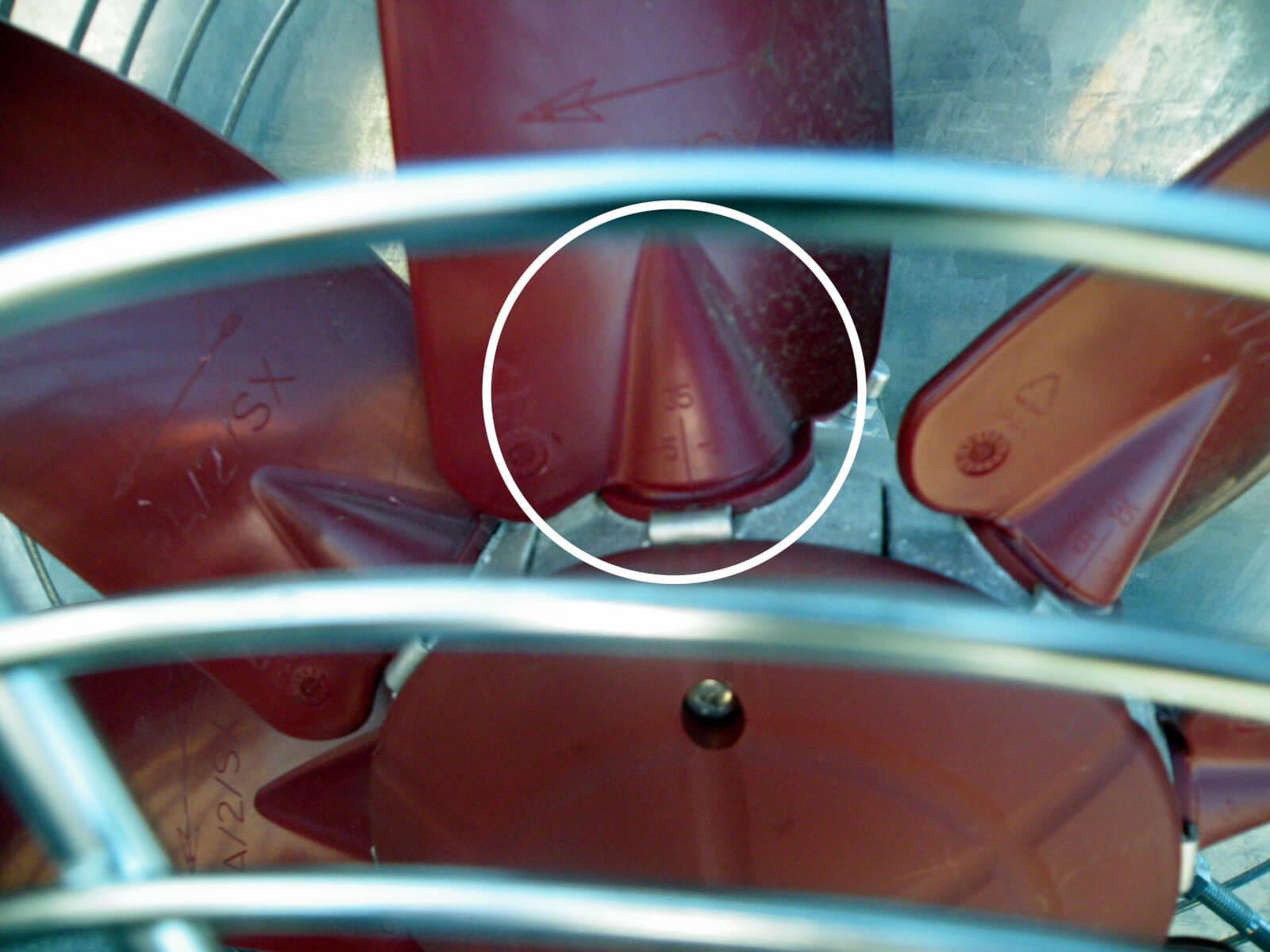
Some airblast sprayers, like this one, feature fan blades with manually-adjustable pitch to increase or lower air volume and speed. It’s often a pain to try to adjust them, and most operators only try it once.
A good time to try this out is early in the spraying season when (most) canopies are dormant and at their most sparse. For example, when applying dormant sprays in apple orchards, look to see if the wood on the sprayer-side gets wet, but does not creep around the sides. This suggests that the air, and much of it’s droplet payload, are being deflected. When the air speed is slowed, it will become more diffuse and turbulent on target surfaces, and this turbulence helps more droplets deposit in a panoramic fashion within (not past) the target canopy. Look to see if the wood is wet >50% around the circumference of the branches. You’ll get the rest when you spray form the other side.
Limitations
GUTD is not always appropriate. It requires airblast sprayers with PTO-driven positive displacement pumps (e.g. diaphragm). Airblast sprayers with centrifugal pumps would experience a drop in operating pressure and would have to be re-nozzled. Further, the pump must have sufficient surplus capacity to maintain pressure at low rpms.
GUTD is not intended for air-shear sprayers that employ twin-fluid nozzles because dropping air speed below a certain threshold may compromise spray quality; the air needs to be fast enough to create and direct spray droplets
The tractor must have sufficient horsepower (more than 25% in excess of minimally-required capacity) to permit the reduction in engine torque. This is especially important if the operator is on hilly terrain. If the tractor begins to lug (e.g. black smoke, sluggish response, strange sounds) you’ll be in trouble.
Observations
We first experimented with GUTD in 2013. We noticed how much quieter the sprayer was, and the fuel consumption was certainly reduced. One grower-cooperator switched to a GUTD spray strategy mid-way through their dormant oil application in pears. We saw the trees immediately began to drip. Panoramic coverage was improved significantly; once the operator passed down the other side of the target, capillary action and surface tension helped to give near-complete coverage.
However, in one instance, the operator was already applying a low spray volume per hectare using air induction nozzles and their lowest fan gear. By further slowing fan speed using GUTD, coverage at the top of his cherry trees was compromised.
In short, GUTD can work under the right circumstances. If you want to try it, use water-sensitive paper to establish a base-line with your current practice, and then evaluate coverage after you change your sprayer settings.
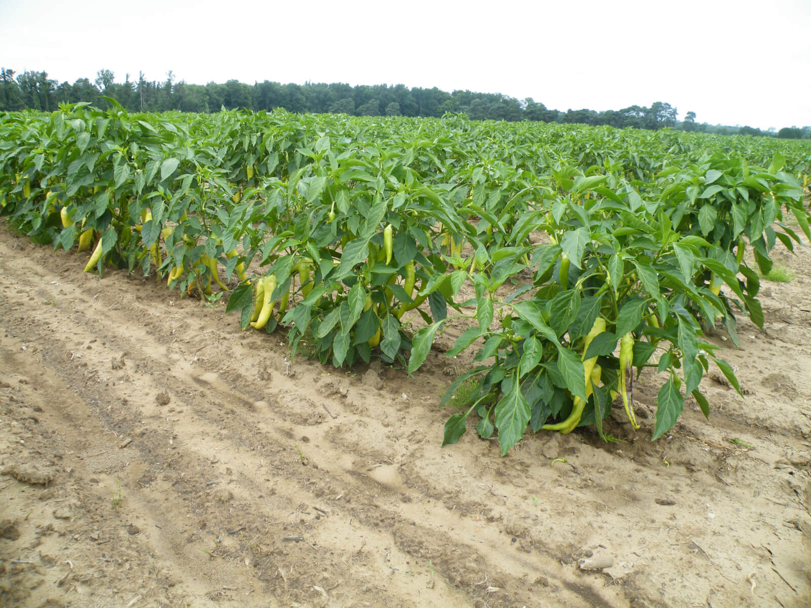
In early July 2016, a farm supplier contacted us on behalf of a client with a history of disease control issues in his field pepper operation. He wanted us to calibrate their sprayer and diagnose spray coverage to see if there was room for improvement. Improved coverage doesn’t necessarily mean improved efficacy, but generally it’s a reliable indicator. When we arrived at the field the winds were gusting over 15 km/h, which had the potential to create a massive drift issue. We were only spraying water, so it was decided that if we managed decent coverage in those conditions, there would be no need to worry on an acceptable spray day.
Field pepper in Southern Ontario in mid-July
The grower traditionally ran two different settings on his sprayer. They were relatively low volumes for a vegetable operation, but the crop was still small at this stage, so we did not propose raising the volume:
TeeJet AITX 11008’s on 50 cm (20″) centres at 11.25 kmh (7 mph) and 3.44 bar (50 psi). That’s 3.35 L/min (0.89 gpm) per nozzle for a total rate of 350 L/ha (37.5 gpa).
TeeJet ConeJet TXVK18’s on 50 cm (20″) centres at 7 kmh (4.5 mph) and 3.44 bar (80 psi). That’s 1.6 L/min (0.42 gpm) per nozzle for a total rate of 275 L/ha (29.5 gpa).
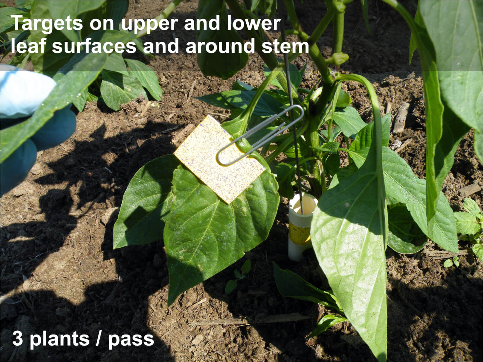
To test the coverage with these settings, we folded a piece of water-sensitive paper over a leaf to cover both surfaces, and wrapped one around a hollow tube to mimic a plant stem (see figure). Three plants were papered for each sprayer pass. Papers were collected, digitized and analysed for percent-coverage and droplet density. When diagnosing coverage for a horticultural crop, a distribution of 85 medium deposits/cm2 and 10-15% coverage is a reasonable standard for most applications.
Location of water-sensitive papers in situ.
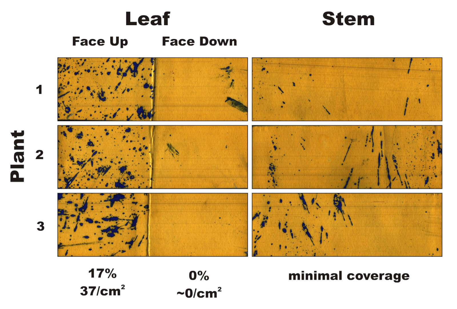
The first condition (the AITX tips) averaged 17% coverage on upper leaf surfaces (37 deposits/cm2). These were coarser droplets at relatively low volume, so it was no surprise that we didn’t achieve 85 deposit/cm2 target. When using such large droplets, it is more important to achieve an even distribution and the 10-15% surface coverage (we achieved 17%). There were no deposits on the underside of the leaves (See figure 1), but that was also expected as coarser droplets tend to follow a downward vector that is not conductive to under-leaf coverage.
Figure 1 – Water-sensitive papers from three plants sprayed in Condition 1. Percent coverage and droplet density are calculated for the leaves, and a visual inspection is made of the stems.
The second condition (the ConeJets) provided better coverage. The fine droplets produced covered an average 17.5% coverage with a distribution of 99 deposits/cm2 on upper surfaces, and 23% coverage with a distribution of 185 deposits/cm2 on lower surfaces. Panoramic stem coverage was improved as well (see figure 2). This is excellent coverage, but the finer droplets were highly prone to drift (see below). With no form of drift control, this set up is undesirable.
Figure 2 – Water-sensitive papers from three plants sprayed in Condition 2. Percent coverage and droplet density are calculated for the leaves, and a visual inspection is made of the stems.With no form of drift control, the finer droplets produced by hollow cones create unacceptable spray drift, even in moderate wind conditions.
This led us to propose a more directed boom arrangement: We set up a hollow cone over the row (the grower’s original ConeJet) and a drop hose suspended in each alley with two TeeJet XR 8004 flat fans positioned on an angle (i.e. not vertical or horizontal to ground). This gave sufficient height to span the canopy with as little direct waste on the ground as possible. As the crop grows, the nozzles would need to be twisted into a more vertical alignment.
ConeJet TXVK18’s alternating with drop hoses with TeeJet XR 8004’s.
We did not use an air induction fan to avoid the Very Coarse spray quality and we used 80° instead of 110° to ensure the spray did not overshoot or undershoot the plant. Here are the details of the third set up:
3. TeeJet ConeJet TXVK-18’s on 100 cm (40″) centres at 7 kmh (4.5 mph) and 3.44 bar (80 psi). That’s 1.6 L/min (0.42 gpm) per nozzle. Also, two TeeJet XR 8004’s per drop on 100 cm (40″) centres at 7 kmh (4.5 mph) and 3.44 bar (80 psi). That’s ~4.5 L/min (1.2 gpm) per drop hose. Together, set of nozzle for a total rate of 523 L/ha (56 gpa).
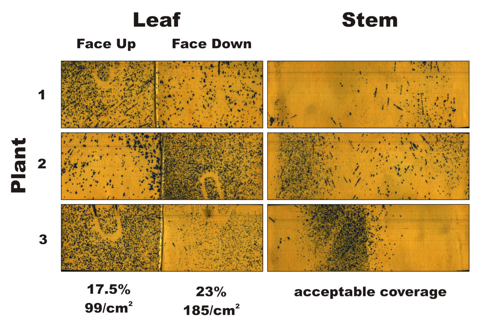
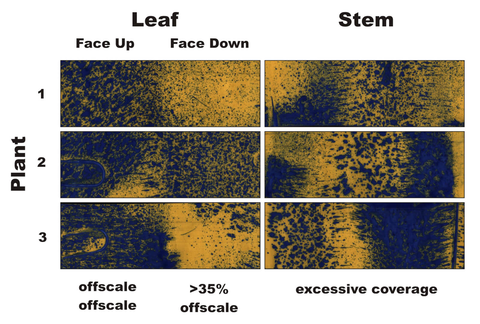
This set up raised the volume considerably and aimed spray directly at the sides of the plant. Coverage was excessive and in a few cases exceeded what the diagnostic software could reliably resolve (see figure 3). Since the plants were still small at this stage, it was decided we would let them “grow into the volume” and come back to check coverage once they were at full size.
Figure 3 – Water-sensitive papers from three plants sprayed in Condition 3. Percent coverage and droplet density are calculated for the leaves, and a visual inspection is made of the stems.
When we returned in mid-August the plants had reached full maturity. In this final coverage trial, we added a second water-sensitive paper to each plant to span the height of the crop canopy, which had grown considerably.
The same pepper plants ~5 weeks later had more than doubled in size.
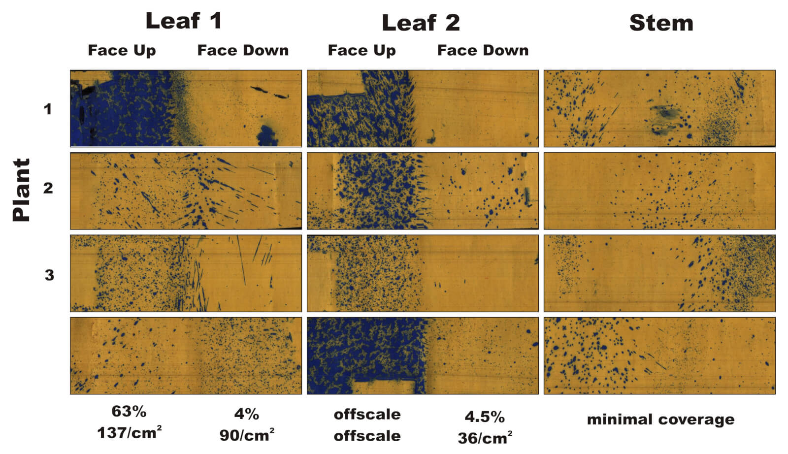
Coverage was reduced compared to how we left things in July, but appeared to be sufficient on key surfaces (see figure 4). The papers showed upper leaf-surface coverage of 63%-to-offscale and deposit distribution of 137 deposits/cm2-to-offscale. Coverage on the lower leaf surfaces was greatly reduced to 4-4.5% and 36-90 deposits/cm2. Panoramic stem coverage was present, but minimal. Applying higher volumes would likely have improved matters.
Figure 4 – Water-sensitive papers from three plants sprayed in Condition 3, ~5 weeks later. Percent coverage and deposit density are calculated for the leaves, and a visual inspection is made of the stems.
When asked about the drop hoses, the grower reported “They are a bit of a nuisance because they take extra time to put on, and they get caught in the bush at the back of the field. But if they increase our coverage, then they’re worth the extra effort.”
Final thoughts
Adding drop hoses to a vegetable sprayer may be unconventional, but if fungicide coverage is a concern, and the drops will fit between rows, they might be worth a try. Carefully consider the volumes you use because they should reflect the size of the plant canopy you are trying to protect. Finally, water-sensitive paper provides excellent feedback to help you decide if your field volume, nozzle rates and nozzle positions are providing acceptable coverage.
We’ve heard it often: calibrate your nozzles to be sure your boom output is uniform across its entire width. The downside of poor uniformity is obvious: strips of over- or under-application causing problems with pest control or crop tolerance. A graduated cylinder held for 30 s under each nozzle is the approach of choice. Several electronic versions exist to make the job easier, for example the Spot On.
But there’s more to the story. Nozzle calibration only ensures volumetric uniformity from nozzle to nozzle. It serves to identify worn, plugged, or damaged nozzles, and little else.
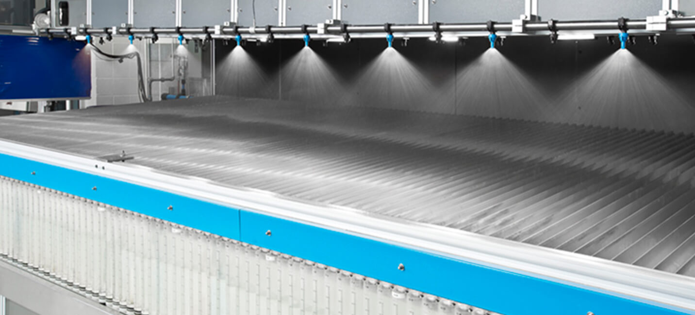
After release, the spray is atomized and distributed across a wider area with a properly developed pattern. An operator adjusts boom height or spray pressure to generate proper overlap for a given fan angle at the target height. Unfortunately, the uniformity of this pattern can’t be measured with a graduated cylinder, so we’ve traditionally used a “patternator”, a flat collector placed under a few nozzles that uses a series of channels to show the peaks and valleys of the volumetric distribution. Both calibration and patternation are done with a stationary spray boom. Nozzle manufacturers employ both methods to ensure their products meet international uniformity standards before marketing.
A spray patternator determines the uniformity of a stationary boom’s spray distribution (Photo: TeeJet)
Burt even that isn’t enough. We can have good volumetric distribution but still have inconsistent coverage in places. To identify those regions, we need a way to measure small amounts of spray deposit under a moving boom, ideally in the canopy we intend to treat. Here we have a few options. We can place a tracer (dye, salt, etc.) in the tank, and collect spray on small collectors placed throughout the area to be treated. We collect the samples, wash them, and analyze the solvent for the tracer. This requires special equipment and takes time. It’s useful, but only measures dose, not droplet size or density.
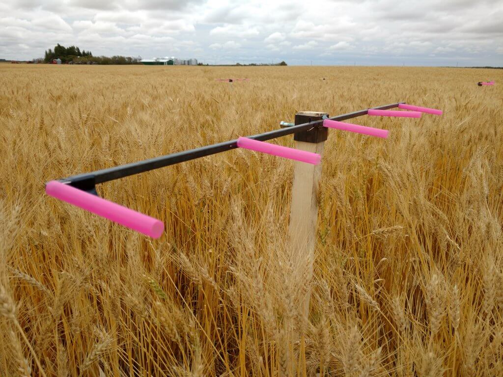
Plastic straws can act as collectors of sprays under field conditions.
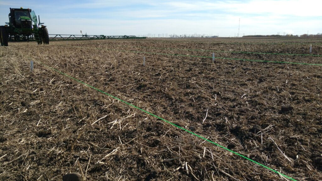
Monofilament strings can be used to collect spray over long distances.
A faster way is to use water-sensitive paper, about which we’ve written here and here. Using WSP is fast and easy, and it can provide additional information such as the number of droplets per unit area, or the total percent of the area covered, or even the size of the deposits, with the right equipment. We call this “coverage”, and believe this to be one of the two components of good pest control (the other being “dose”, the total amount of material deposited). Because the world isn’t fair, WSP isn’t great at quantifying dose.
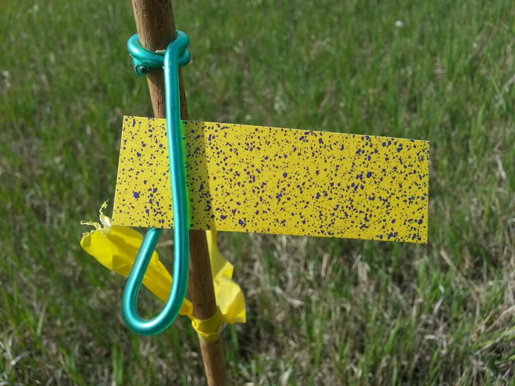
Water-Sensitive paper provides a quick visual indication of the deposit, not just amount but also qualitative aspects such as droplet size and distribution.
The industry has done a good job of identifying the dose required for good control, and this is reflected in the rate recommendations on a label. But there are a few gaps. They don’t tell us, for example, what “good coverage” is, despite often telling us to “ensure” it.
Back to Deposit Uniformity
We quantify deposit uniformity by calculating the Coefficient of Variation (CV) of a series of measurements. The CV is defined as the standard deviation of these measurements, expressed as a percent of the mean value.
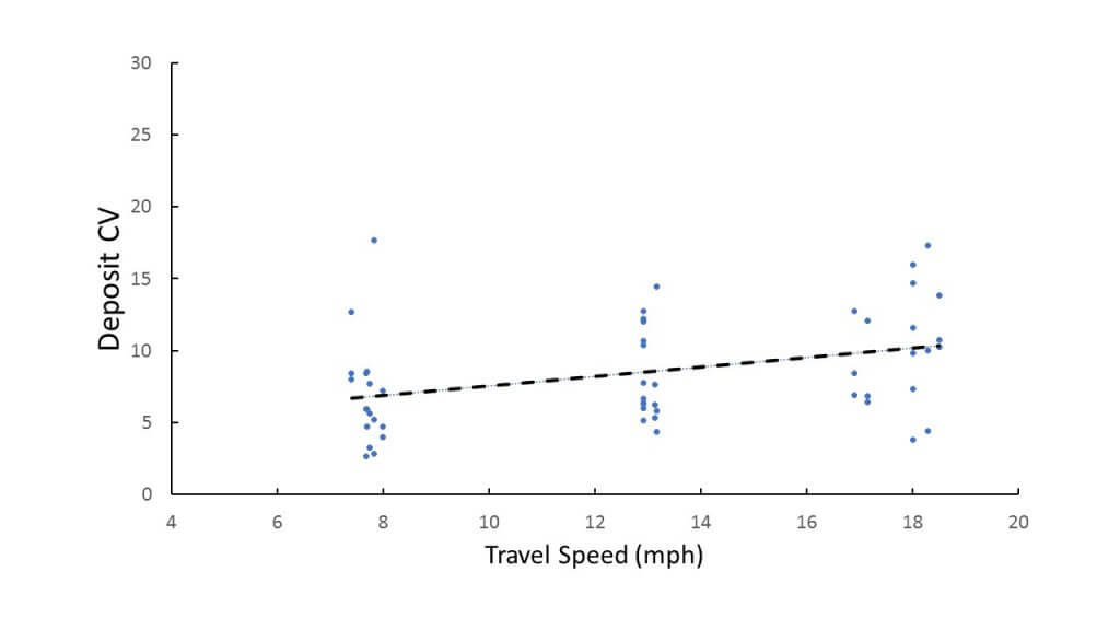
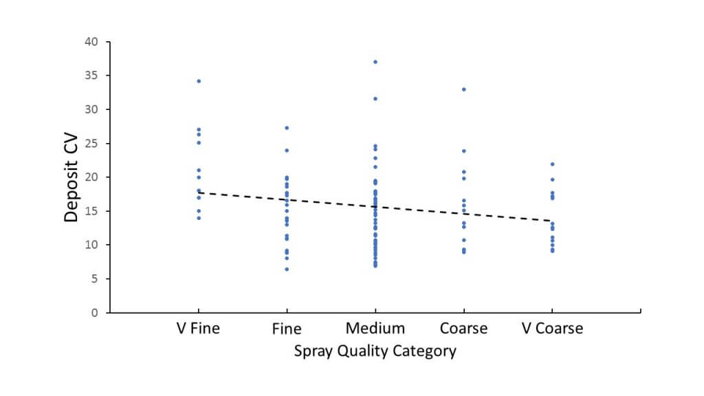
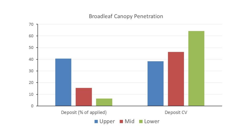
Because it’s hard to measure, it’s easy to ignore. But here are a few basics our research has told us: (In the first three examples, deposits were measured under a spray boom using petri plate or drinking straw samplers. There was no interference from a canopy. The last example was taken from within a canopy.)
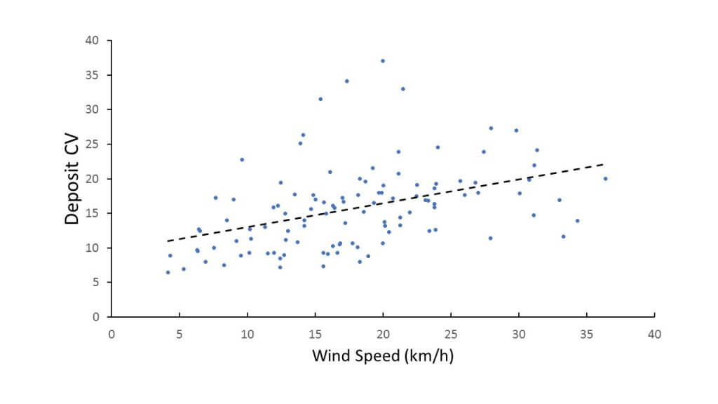
When measuring the deposited dose, the CV under a boom tended to rise with increased wind speed. This is no surprise, as it reflects that more wind has a greater chance to displace spray from its intended destination.
Spray deposit uniformity, observed during various spray drift studies, tended to decrease with higher wind speeds.
Higher booms and increased travel speed also tended to increase deposit CV.
Faster travel speeds during spray drift studies tended to decrease uniformity.
Finer sprays tended to increase deposit CV. This makes sense, as the finer droplets are more easily displaced by air movement.
Coarser sprays created more uniform deposits possibly because they were more resistant to turbulent displacement.
Deposits were reduced and became more variable deeper in a broadleaf canopy. Again this makes sense, as there are a lot of obstacles to clear and canopies themselves are by no means uniform.
Deposit amount was lower in the canopy, as expected. But the lower deposit was also more variable.
Also note that the CV in the canopy was quite a bit higher (40 – 60%) than for the exposed targets (10 – 20%). That’s another challenge.
To recap, the best uniformity was achieved with low booms (as long as patterns overlap sufficiently), slow speeds, low winds, and coarser sprays. It’s easy to see that current spray practice isn’t always conducive to uniform deposits.
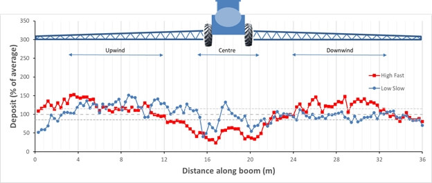
Deposit variability as captured by a 2 mm diameter string with two sprayer configurations.
So What?
Why does uniformity matter? It matters because more variable deposits are less efficient. They require higher doses for the same effect as uniform deposits. Here’s why:
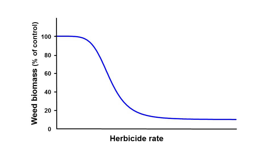
The figure below shows a typical dose response curve for a herbicide. On the y-axis, we see weed biomass, on the x-axis herbicide dose. At low pesticide doses, not much happens. (In fact, we often see a slight increase in biomass with very low herbicide doses.) As we increase dose, biomass begins to decline, and as dose increases further, the effect begins to taper off. At a certain dose, no further biological response is possible.
A typical dose response curve for a herbicide.
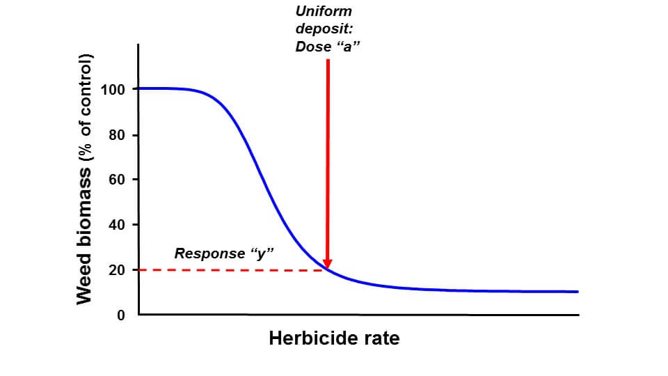
In the next figure, we see that application of a uniform dose “a” results in biomass “y”, about 20% of untreated.
A dose response curve represents the weed biomass that resulted from any applied dose.
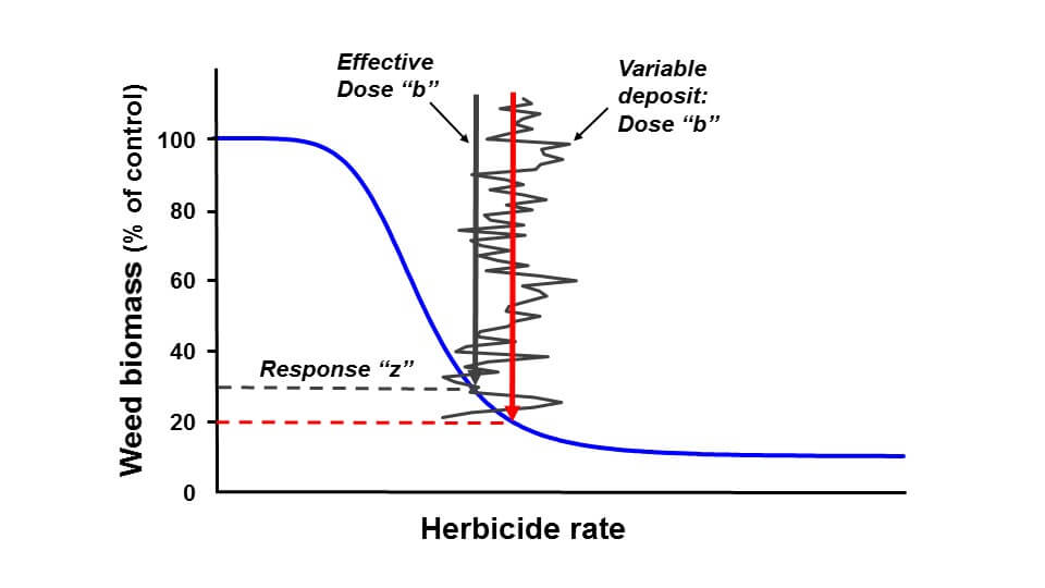
Next, we apply the same average dose, but we do it non-uniformly. At some locations under the boom, the deposit may be 40% higher or lower than average. The result is response “z”. Weed control is worse, as bad as it would have been at a lower uniformly applied dose (effective dose “b”).
A variable dose across a field results in many individual weed biomasses because of deposit variation. The net result is lower control.
This effect only happens when the effective dose is near the lower inflection point of the dose response curve. Perhaps we’re shaving rates. Perhaps the weather is challenging the herbicide’s performance. Or perhaps the weed is difficult to control. Under those conditions, any gain in performance with a higher dose is less than the penalty from a lower dose.
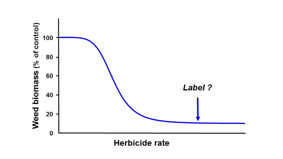
There are two ways to correct this performance loss. One is to apply a higher herbicide rate. It’s commonly done, as insurance against – you guessed it – variability, and it’s one reason why label rates have some flexibility. The second way is to improve deposit uniformity. In effect, better uniformity allows for rate reductions.
Label rates are typically in the flat region of the dose response curve to allow for variable conditions in weed susceptibility, weed growth stage, growing conditions, and deposit variability.
Take Home Message
Uniform spray deposition improves overall control. Our examples used herbicides, but the same is true for fungicides and insecticides. It’s true for field crops as well as fruit and vegetable sprays.
Uniformity is especially important when the application is done under adverse conditions in which the pesticide performance is challenged. It’s a fundamental part of good application practice.
It’s not always easy to improve uniformity. But at least it should be measured. Without measuring it, an applicator may never know how much product is being wasted. Have a look at the Crop Adapted Spraying approach Jason is using, it’s a template for all sorts of applications.
What can you do? The easiest task is to record the flow from each nozzle. The results might be surprising. Ensuring proper and consistent boom height is also important. Using water-sensitive paper to visualize the quality of the job would be icing on the cake. And adjusting application method, with uniformity as a goal…that gets you a gold star.
When we consult a nozzle catalogue we are interested in the flow and droplet sizes produced at a given pressure. Perhaps we should also consider the effect of pressure on spray angle. We have several articles discussing the collective impact of spray overlap, nozzle spacing and boom height on coverage uniformity (Check here and here for example). However, we don’t really address the fact that fan angle is not a constant. This may be more relevant with the growing adoption of spot sprayers.
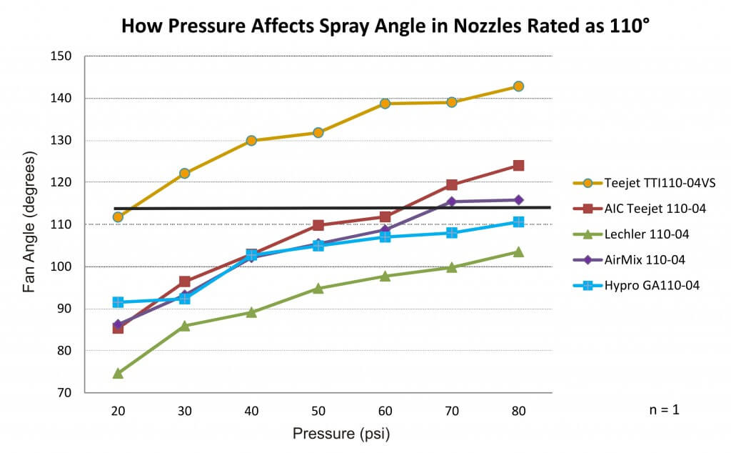
To illustrate the potential for fan angle variation, we assembled a collection of red, flat fan nozzles (‘04s) from several manufacturers. We plugged each nozzle into a spray pattern table, set the regulator at a given pressure, and photographed the spray angle and flow distribution. This process was repeated for each nozzle at seven different pressures within the manufacturer’s approved range of 20-80 psi. After digitizing the photos, we measured the spray angle using a digital protractor.
We anticipated a concomitant increase in spray angle as the pressure increased. This is not news. Anyone who has operated a sprayer has seen the spray pattern open up as the boom fills and pressurizes. Bear in mind this was only performed once (i.e. n=1), so while it illustrates trends it shouldn’t be mistaken for a rigorous scientific comparison. Further, this demonstrates a static situation and not a dynamic one where travel speed, wind conditions and the vortices from the sprayer it self will influence matters.
We saw similar trends with nozzles other than 110˚ fans, but let’s focus on 110˚s due to their current popularity.
Fan angles for five common 110 degree AI flat fans over their manufacturer-recommended pressure range
The spray angle for 110˚ nozzles ranged from 75˚ at 20 psi to approximately 143˚ at 80 psi. One nozzle failed to reach 110˚ at any pressure. Conversely, there was another that was over 110˚ at nearly all pressures. Ideally, spray nozzles should be operated around the middle of their manufacturer-recommended operating range. Three of the nozzles tested came close to 110˚ at that median pressure, but only the TeeJet AIC110-04 measured 110˚ at the middle of its recommended range (~50 psi).
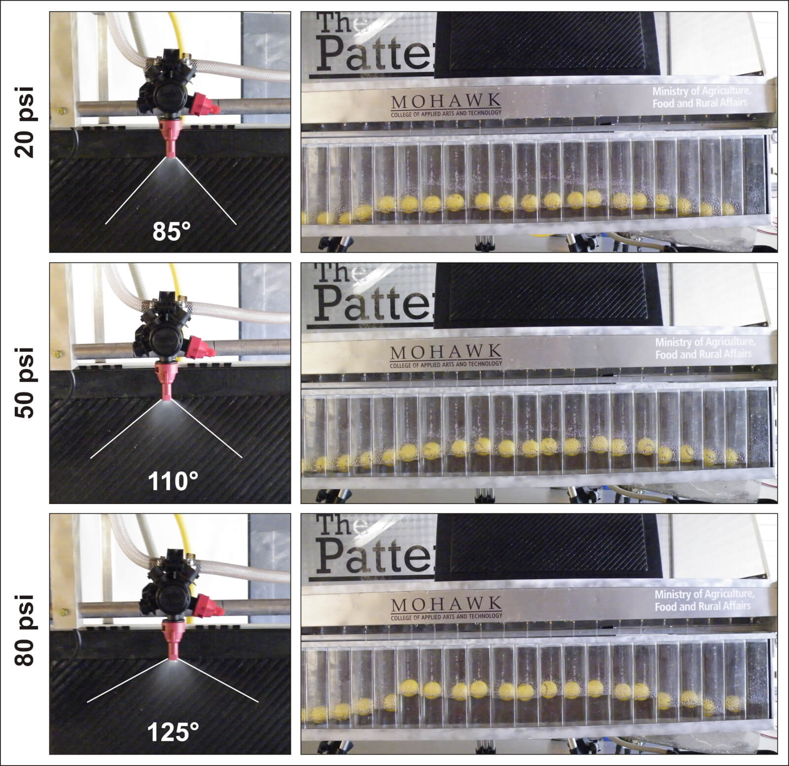
Using that nozzle as an example, let’s look at the pressure, spray angle and subsequent distribution of flow along the swath at three different pressures. At 20 psi, the spray angle was 85˚. The yellow balls are floats that reflect flow as a series of cross sections of the swath. We see that aside from the tapered edges (which illustrate the need for 100% overlap between neighbouring nozzles) the distribution was fairly even. One of the priorities in nozzle design is to ensure a low coefficient of variability over the operating pressure range. In other words, the length of the swath may change, but the spray quality and uniformity in that swath is still within spec. At 50 psi the nozzle produced the expected 110˚ fan, and the spray distribution remained even. At 80 psi, the angle spread out to 125˚, spanning a greater distance, but it started to produce a less-even distribution.
Photographs of spray angle and distribution for the TeeJet AIC110-04 at the extreme low, middle and highest pressures of its recommended pressure range.
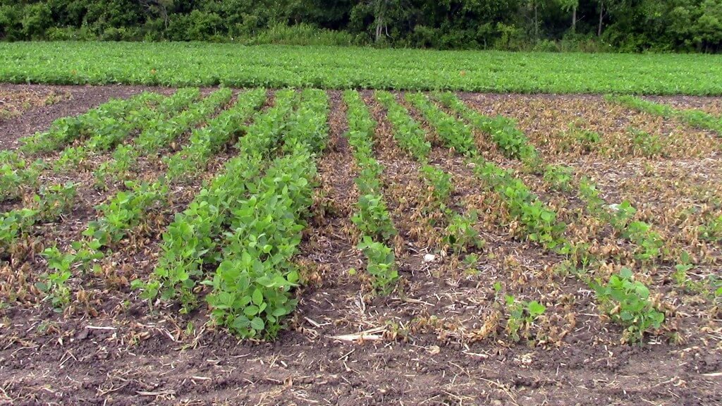
When fan angle changes with pressure, it can have significant implications. Nozzle spacing on a boom varies from sprayer to sprayer. Generally 50 cm (20 inch) centres are the standard in North America, but we’ve seen 15″ and even 10″. Nozzle spacing and boom height collectively determine the degree of spray overlap. Excessive overlap isn’t a problem, although additional nozzles do mean added expense, cleaning time and potential for plugging. Conversely, gaps in the pattern could lead to sub-lethal applications or flat-out misses. For example, in this soybean demo plot (below) we sprayed a contact herbicide at low pressure to collapse the spray pattern. You can see the alternating stripes of hits and misses that resulted from an incomplete overlap of spray.
Soybean demo plot sprayed with a contact herbicide using 110˚ air induction flat fans at 20 psi. The collapsed spray pattern did not overlap sufficiently to burn the entire crop down, leaving a striped pattern and demonstrating the poor coverage.
Nozzle manufacturers generally recommend a 100% spray overlap for flat fans. This creates sufficient overlap when the boom sways low to the ground. It also increases the degree of droplet size homogeneity under the boom as coarser and fewer droplets are generally found at the “horns” or edges of the pattern compared to the centre. In order to ensure this degree of overlap, sprayer operators should observe and consider changes in fan angle over their typical pressure range. Otherwise, the cost of poor deposit uniformity under the boom could be high.
Operate nozzles around the middle of the manufacturer-recommended pressure range. However, just because a nozzle is rated over a range of pressures does not mean the angle is constant.
Lower pressures are a greater concern than higher pressures. 30 psi is the absolute lowest pressure for operating a 110˚ air induction flat fan; the ideal operating range for these nozzles is 50-70 psi.
If nozzles are not maintaining the recommended 100% overlap at your preferred pressure range, then consider switching nozzle rates, and adjusting pressure and boom height.
This work was performed with Victoria Radaukas, 2015 OMAFRA application technology summer student.
If you’re a sprayer operator with some experience behind you, you may have applied mercury arsenate, nicotine, Paris green, or perhaps even DDT. All of these historical pesticides were effective, but they were also toxic to both the applicators and the environment. Fortunately, today’s agrochemical manufacturers produce pesticides that are effective while being far less hazardous.
One important aspect of modern synthetic pesticides that enhances their efficacy is their ability to redistribute. Pesticide redistribution is the movement of a pesticide from its initial point of deposition to a different spot on or in the plant. Pesticides that can redistribute can improve pest control compared to those that must contact the target pest but cannot innately redistribute. This is especially true when spraying hard-to-wet plant tissues, such as flower clusters or fruit. Even when the immediate coverage of these tissues is insufficient, the subsequent relocation beyond the initial spray deposit can result in a more effective protective barrier. When plants are rapidly growing, many of these products can translocate through the plant tissues to protect newly emerged tissue that did not receive a direct deposit.
Some of the most difficult and persistent pests are more effectively controlled by redistributing pesticides. Materials that move within the plant after application provide improved control of piercing-sucking insects such as aphids and psyllids, as well as pests that feed in difficult-to-spray areas such as under leaves. These products can absorb into plant tissue, increasing their resistance to wash-off by rain or irrigation.
Five Types of Pesticide Redistribution
There are five significant types of pesticide redistribution: translaminar, vapor, xylem, phloem and redistribution via precipitation
Translaminar Redistribution
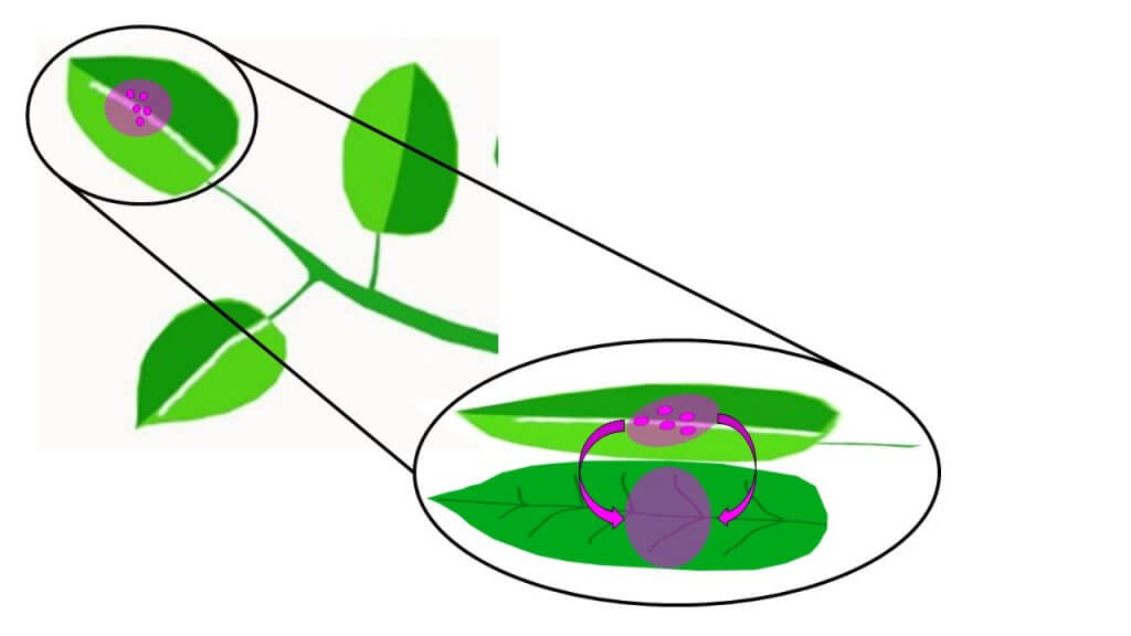
Translaminar redistribution (Figure 1) in its most literal sense is a compound moving from the side of the leaf that received spray, to the unsprayed opposite side. This results in protection on both sides. However, translaminar redistribution also involves limited radial movement providing a “halo” of protection around the initial deposition. The extent of this area of influence is product-dependent.
Figure 1. Schematic of translaminar redistribution, with small round dots indicating deposition of pesticide, arrows indicating the direction of redistribution, and the shading indicating the area of the plant protected by the pesticide.
Vapor Redistribution
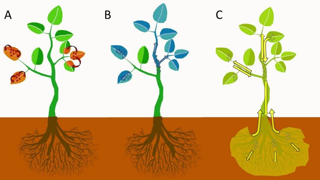
Vapor redistribution (Figure 2A) occurs when surface depositions volatilize and move laterally along a plant surface, re-adsorbing to the plant surface in new locations as they move. Again, the extent of vapor activity is product specific, but also condition specific requiring an optimal combination of temperature, relative humidity, wind, and solar radiation to facilitate volatilization. When pesticides are referred to as “locally systemic,” it often implies that they exhibit translaminar and/or vapor redistribution properties.
Figure 2. Pesticide redistribution type schematics (A) vapor, (B) xylem, (C) phloem. The small colored groups of dots indicate deposition of pesticide, while arrows indicate the direction of redistribution, with shading representing the area of the plant protected by the pesticide.
Xylem and Phloem Redistribution
Xylem redistribution (Figure 2B), also called xylem systemic, refers to the absorption of a pesticide and subsequent systemic movement of the pesticide through the xylem vessels of a plant. Xylem vessels move water and minerals in an upward and outward direction in plants. There is very little movement of water and nutrients downwards or backwards along branches or leaves in xylem vessels. Xylem redistribution can help protect growing tissues from damage by pests or diseases when the pesticide redistributes from the point of application to the newly developing tissues. Most systemic fungicides and insecticides redistribute via the xylem.
Phloem redistribution (Figure 2C), also called phloem systemic, is the bi-directional movement of pesticides in the phloem vessels of a plant. Phloem vessels transport sugars and other nutrients both to the roots of plants and upwards and outwards to shoots and fruits/seeds. Phloem systemic pesticides are sometimes called “true systemic,” because they can translocate throughout the entire plant.
Some pesticides that redistribute via the xylem or phloem can be applied to the soil substrate to be absorbed by the roots and redistributed throughout the plant. The process of plant nutrients or pesticides being transported from one place to another within the plant is called translocation.
Soil-Applied Systemics
Several factors affect a pesticide’s ability to redistribute. These factors affect the speed of uptake, the duration and extent of translocation, and the amount of accumulation in plant tissue relative to the initial dose. For pesticides labeled for soil application, their uptake by plant roots and redistribution via xylem or phloem can lead to long residual efficacy of the product; Up to eight weeks or more depending on the product, plant, and soil. This is in contrast to foliar-applied products, where good residual efficacy could be expected to last two to three weeks depending on the product. However, foliar-applied products tend to provide a more rapid kill of target pests and a more rapid absorption and translocation of active ingredients.
For soil-applied systemic pesticides, the composition of the soil substrate can affect the uptake of the pesticide by the plant. Growing media high in organic matter (>30% bark or peat moss) can bind pesticides, making it difficult for plants to absorb them through roots and subsequently translocate via the plants vascular system. Soil applications of systemic materials should take place one to six weeks prior to the onset of the insect pest or pathogen. This allows sufficient time for the pesticide to translocate to, and accumulate in, target tissues. The more water-soluble pesticides (e.g. Thiamethoxam) are taken up more rapidly than the less water-soluble pesticides (e.g. Imidacloprid).
Redistribution via Precipitation
In contrast to systemic pesticides, contact pesticides cannot redistribute on their own. However, rain or irrigation can spread the deposit to some degree, increasing coverage area. This effect should not be relied upon, as it depends on the product formulation, the intensity of the precipitation, and the interval following application. In the case of prolonged precipitation, the residual activity of contact products can be greatly reduced as they are diluted and washed off plant tissues.
Plant Morphology
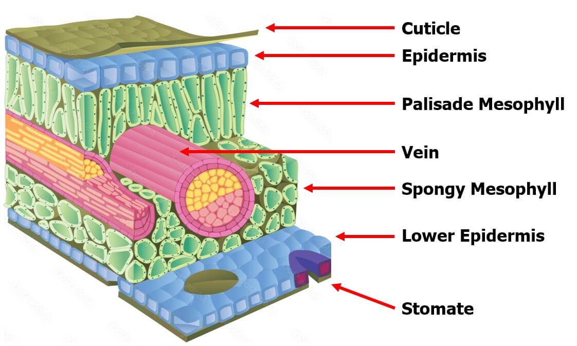
The status of the plant to which they are being applied is a significant consideration when applying redistributing pesticides. Both soil-applied and foliar-applied pesticides are more rapidly absorbed and redistributed when applied to young plants or juvenile plant tissue. In general, when plants are actively growing, have a strong root system, or are actively transpiring, they tend to absorb and translocate pesticides more rapidly than when plants are growing slowly. In addition, plants with difficult to wet leaves or surfaces due to thick cuticles or waxy layers tend to not absorb pesticides as readily. Penetration into plants with difficult to wet surfaces can be improved by adding adjuvants such as surfactants to tank mixes.
Multiple Modes of Redistribution
The extent to which each product can redistribute can be thought of as a continuum. Generally, when a product exhibits some form of redistribution, it can also redistribute via a different method. A good example of this is xylem and translaminar redistribution. When a product can redistribute via the xylem it generally can move through the leaf via the translaminar pathway as well. Some products can redistribute via the xylem, translaminar, and vapor pathways all at the same time. Others, while technically able to redistribute via more than one mechanism, are only biologically effective via one mechanism.
Consult the Pesticide Label and Other Reputable Sources
The best way to determine how a pesticide product redistributes is to consult the manufacturer’s label, as well as technical information from reputable sources such as government or academia. If a manufacturer provides a technical information bulletin it is generally available on their website on the pesticide product page along with the label. However, because there are no standardized metrics to rate pesticide redistribution, there can be significant disparity between products. Some products that are advertised as being xylem systemic for example, are actually less systemic than products that are not even advertised as being systemic. Additional information on the efficacy and redistributing characteristics of specific products can be obtained from extension agents or crop consultants.
Conclusion
In summary, when selecting a pesticide remember to consider the four different pathways of redistribution (xylem, phloem, translaminar, and vapor) and how these methods may improve the efficacy of your application, allowing you to get more out of every drop.