We’ve often heard the adage “Coverage is King” but what does that mean, exactly? It means that in order for your spray application to yield acceptable results, a threshold amount of the active ingredient in your tank must end up on the target. But at what point have we achieved sufficient spray coverage without wastefully over-applying to the target? What does good coverage look like?
Let’s manage expectations right here at the beginning of the article: There is no single, definitive answer because it depends on the nature of the application. In other words, you have to understand which factors are relevant to your specific situation before you can understand what success looks like.
Let’s highlight some of those factors:
Transfer Efficiency, Catch Efficiency and Retention
This relates to the spray’s ability to span the distance from nozzle to target (transfer efficiency) get intercepted by that target (catch efficiency) and then deposit a biologically-active residue on the target surface (retention).
First, the spray must reach the the target location. This may be the soil, or it might be the underside of a leaf deep in a plant canopy. The degree of success will depend on the droplet size(s), distance to the target and the environmental conditions.
Then the droplets have to be retained by the target surface and not bounce or slide off. Difficult-to-wet surfaces such as fruit, stems and waxy vertical leaves may be more easily covered with finer droplets and/or formulations that include activator adjuvants (e.g. surfactants).
Then the deposit must stay wet long enough to be absorbed by the tissue, or leave a hardy residue on the surface that can withstand weathering (e.g. precipitation, sun, and even bacteria) long enough to encounter the pest. More on this below.
Mode of Action
This relates to where spray must deposit (or relocate to) in order for it accomplish it’s objective. Here are a few examples of how products might work. Read your pesticide label to determine your situation.
Some products require contact. Insects must touch them, either via a droplet landing on them or as they move through a deposit. Similarly, certain fungicides must contact fungal hyphae on the plant surface. A few products are designed to drench the target, as is the case with oil-based miticides.
Some insecticides must be ingested. That may be in the form of a surface deposit or in plant material that has absorbed the chemistry. Similarly, some fungicides are absorbed by plant tissue.
Many herbicides are mobile (i.e. systemic). They may be drawn up through the roots, or enter the cytoplasm via leaves and travel to the growing points on the plants, or move through the xylem. Others are contact, staying relatively close to the original deposit.
The sprayer operator should consider these factors when planning the application and when evaluating the resulting coverage. So how do we visualize coverage? Some operators look for the shine on leaves, or a cloudy residue once the spray has dried. That’s better than nothing, but we recommend water sensitive paper (WSP), which is still the most versatile and economical way to visualize coverage.
WSP can be purchased from most retailers that carry spray equipment. It is available in three sizes, of which the 1” x 3” size is the most common. It can be folded and clipped to a plant surface, or placed on the ground. We’ve written several articles on how to use it (such as here and here and in pretty much a third of the articles on Sprayers101).
There are two metrics that must be evaluated when assessing coverage on water sensitive paper:
the area of the target that has spray on it, and
the distribution of the droplets over that area.
Let’s use a metaphor to explain:
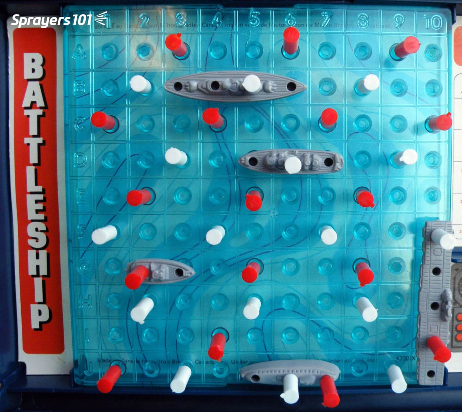
The Battleship® / Coverage Metaphor
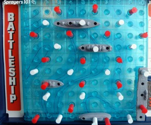
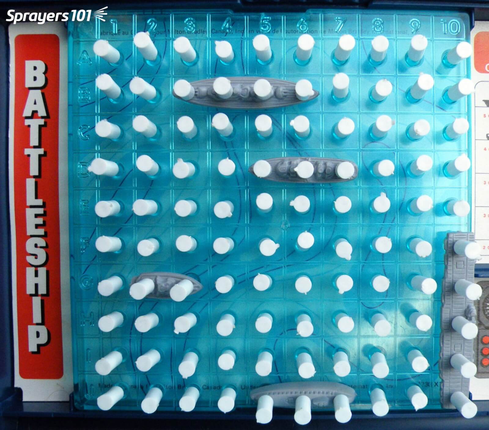
Imagine the boats in this Battleship® game are the insect pests, and the board they’re on is a leaf. The white pegs represent the spray deposits. In this first image, we see 100% coverage and a very high deposit density. Sure, we got every boat, but this is literal and figurative overkill. There’s no need to completely drench the target in order to control most pests. When you spray a target past the point of run-off, you are not adding more pesticide to the target – you are displacing what was already there. The surface will not exceed the concentration of product you sprayed (with the possible exception of mixes that include certain adjuvants). While additional volume can improve coverage to a point, there is a diminishing return.
Unless the label specifically asks for a drench, this is too much coverage.
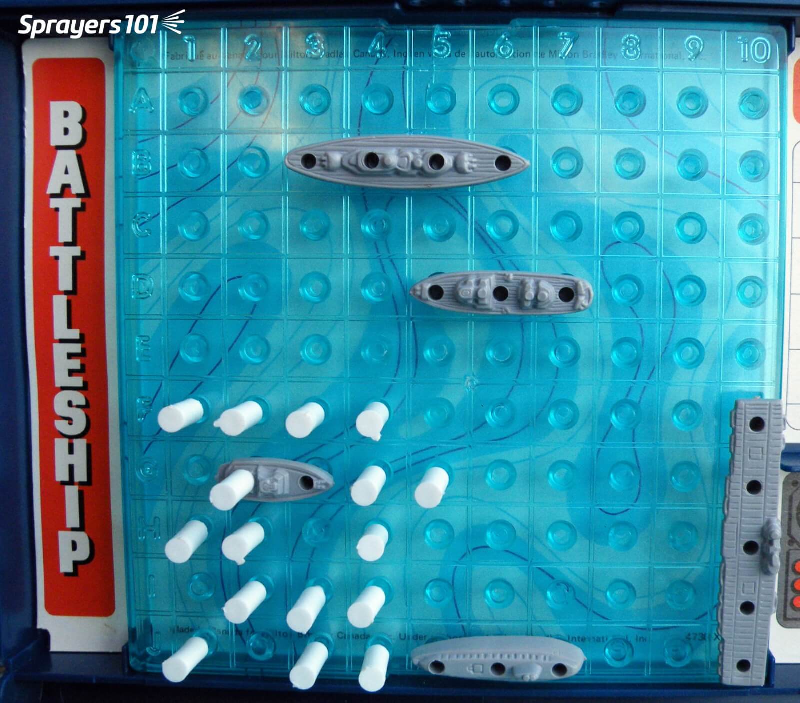
In this second image, we’ve covered about 15% of the target area, which is reasonable. However, note the lack of distribution. You can see that we’ve missed quite a bit of the leaf. If our pretend pests are sedentary and if this was a contact product, then we’ve missed. If this was WSP we would advise the sprayer operator to note how much space there is between the deposits. Could a pest such as an insect or small weed easily fit between the deposits?
15% coverage is good, but the distribution is bad.
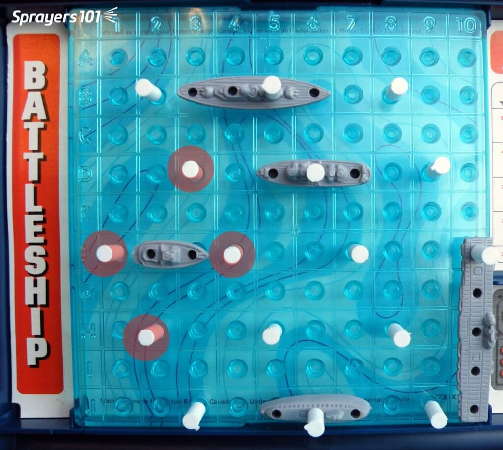
In this third image, we are still covering about 15% of the target, but now the spray is distributed more evenly. Some of you are likely noticing that we missed a pest. That observation reminds me of one of my favourite exchanges from the movie “Christmas Vacation” where Clark finally got his house illuminated, but his father-in-law only sees the problems: “The little lights aren’t twinkling.” “I see that and thanks for noticing, Ed.”
15% coverage, distributed evenly. Deposits may have some pest activity beyond the edge of the residue (light red circles).
Yes, we still missed a pest, but spraying is playing a game of odds. You want enough spray to increase the odds of controlling a pest, but not so much to waste spray (and money and time). This image represents an ideal coverage situation. If this pest moves, or this pesticide redistributes even a little, it will affect the pest.
Plus, we should not discount the threshold of influence that lies around pesticide residue. Imagine a small circle around each droplet (illustrated here as light red haloes) where active ingredient may redistribute beyond the initial deposit to affect an adjacent pest. Perhaps even more importantly, deposits do not spread on WSP the way they do on actual plant tissue, so WSP always gives an underestimate of the potential coverage.
In this last image, we see that red deposits have been introduced. This represents a disease control program where an earlier (white) application retains some residual activity when next application (red) is applied. The second spray application almost never lands on top of the first, giving much more protection on the target. For those keeners out there, note that we got that last pest!
In the case of many disease management programs, subsequent sprays tend to fill in gaps left by previous sprays. If timing is prompt, residual activity will see you through.
If you Absolutely Need a Number…
So, what if you’ve read all this but still insist on a firm number to define adequate coverage? We’ll reiterate that there’s no universally-accepted threshold of deposit density or area covered. It would be nice if pesticide labels included this information, but they don’t.
We’ll stick out necks out and say that in general practice we see excellent results when we achieve 85 discrete deposits per cm2 as well as 10-15% surface coverage on at least 80% of the water sensitive papers in a spray application. If you can manage this, it should give satisfactory results in most situations.
Ontario Agriculture Conference – 2022
For a really in-depth conversation on the topic of coverage, check out our presentation from the 2022 Ontario Ag Conference. We tried to deliver a fun and memorable demo at the end of this presentation to show how different droplet sizes might contribute to coverage. Enjoy.
North American built boom sprayers have nozzle spacings of 20” (50 cm in the rest of the world), but other spacings such as 15” (37 cm) and 10” (25 cm) also exist. What are the reasons for these alternative spacings and do they offer any inherent advantages?
Why spacing matters
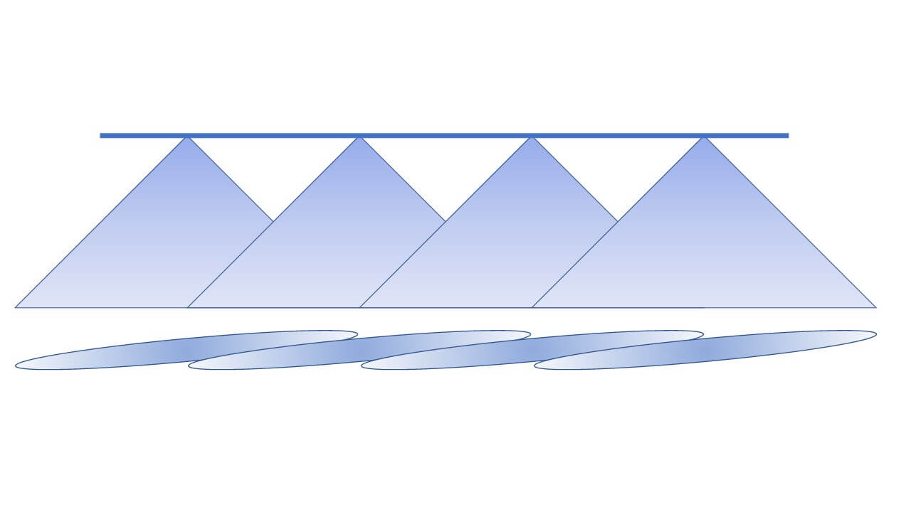
Nozzles are spaced along a boom to allow their fans (patterns) to overlap sufficiently at the target. In broadcast spraying, a uniform distribution of spray volume gives us the best chance for consistent coverage along the boom. Since flat fan nozzles produce a tapered pattern (i.e. the volume is highest in the centre and diminishes towards the edges), approximately 100% overlap (i.e. 50% from each neighbour) will produce a uniform swath.
Figure 1: Tapered flat fans that require some overlap are the default pattern type for agricultural boom nozzles. This is true of conventional and low-drift styles. Note that the flat fans are turned 15° to prevent the spray patterns from interfering with one another.
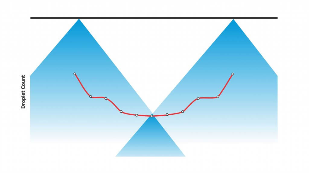
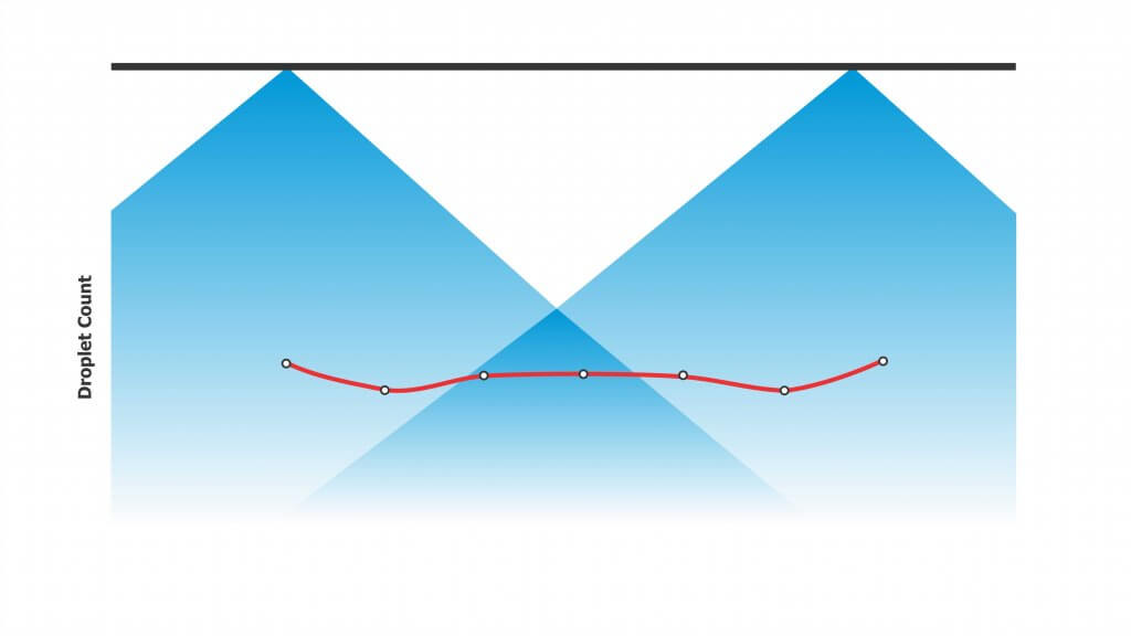
The 100% overlap isn’t just for volumetric distribution. Flat fan spray patterns tend to have more and finer droplets in the centre and fewer and coarser droplets at the edges. All droplet sizes contribute to coverage in different ways, so the overlap ensures both number and sizes are evenly distributed along the entire boom.
Figure 2: 30% overlap may achieve volumetric uniformity. But because the centre of the pattern contains the majority of the smaller droplets, low overlap may result in low coverage in the overlap regions, resulting in striping.Figure 3: Consistent droplet number distribution along the boom requires at minimum 100% overlap (50% from each neighbouring nozzle). This blends those regions of the patterns with high and low droplet densities.
The generic 20” spacing arose from long-held conventions about boom height, fan angle, and travel speed. Specifically, this spacing required a boom height of 20” to obtain good overlap of the once-dominant 80° fan angle. Combined with 0.15 to 0.3 US gallon per minute (gpm) nozzles and travel speeds of 6 to 8 mph, operators were able to apply 5 to 15 US gallons per acre (gpa) volumes. Using nozzles with smaller flow rates would generally result in nozzle blockages.
But what if we want to change any of those variables? How does this affect nozzle spacing? Figuring out the pros and cons of an alternate spacing requires a little math and some contingency management.
Boom Height Math
First the math. If the boom has 20” nozzle spacing and we need 100% overlap, the width of the spray pattern at target height must be two times the nozzle spacing, which is 40″. You must calculate the required fan angle and boom height to achieve this. Most nozzle catalogues have tables to help with this, or you can download a handy spreadsheet to calculate your own scenarios here.
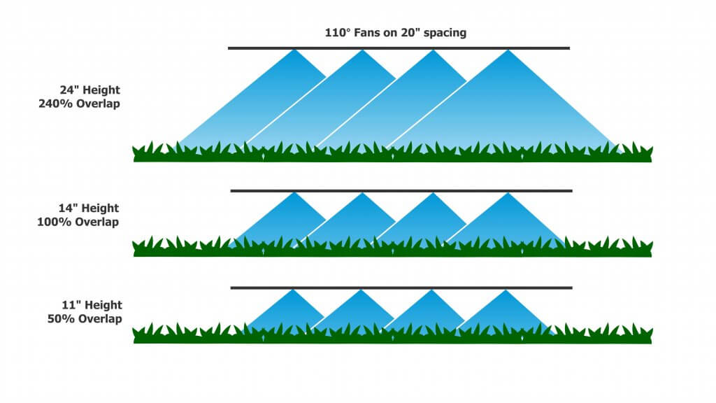
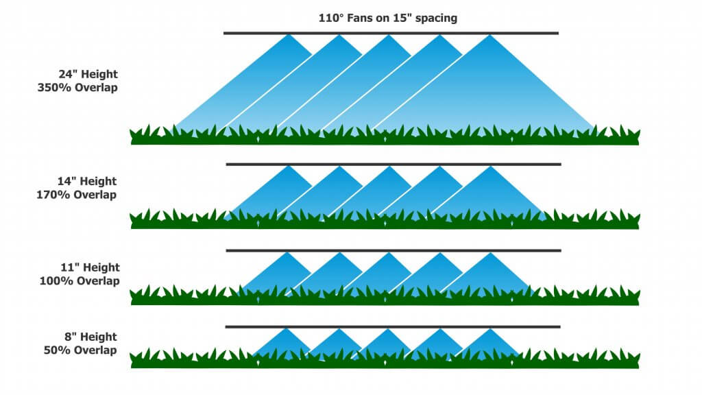
For today’s standard 110° fans, a minimum boom height of 14” is needed to achieve 100% overlap. For 15” spacing, the height is reduced to 11”. For 10” spacing, we drop to a mere 7”. However, consider that most modern suspended booms are not operated at heights less than 24” to allow for sway. At that height, there’s plenty of overlap to go around for 20″ nozzle spacing. For those booms that are able to operate at a consistent height, narrower spacings permit lower heights that will reduce drift potential significantly. Every time we halve boom height, we also halve drift potential.
Figure 4: Using 110° tips with 20″ spacing, the theoretical height at which we achieve 50% overlap is 11″ above target.
By tilting the nozzles forward or backward from the vertical, we can reduce the boom height somewhat further and still get the same overlap. For example, for 20 and 15” spacings, angling nozzles forward or backwards by 30° allows us to drop the boom another 2” closer to the target.
Contingencies
A suspended boom hardly ever stays at a uniform height; It sways up and down with field conditions, topography, etc. This is why many operators set their booms above the minimum height – to prevent striping when the boom sways low. The penalty is that this increases the distance droplets need to travel, increasing drift potential and any turbulent displacement problems arising from the moving boom.
Assuming a 110° flat fan at 24” boom height, each nozzle achieves a theoretical pattern width of about 70”, which is an overlap of 70÷20=3.4-fold or 240% on 20” nozzle spacing. Given a minimally-acceptable overlap of 50% (25% from each neighbouring nozzle), the boom could be as low as 11”. For 15” spacing, the minimum height for 50% overlap is 8”, and for 10” spacing it’s 5”. This means the narrower spray patterns gain 3” to 6” in allowed downward boom movement.
Figure 5: Using 110° tips on 15″ spacing, the height for 50% overlap is 8″ above target.
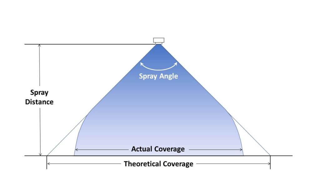
A second contingency is that spray patterns are rarely the exact value that the nozzle catalogues specify. A so-called 110° nozzle may operate at only 90°, or up to 150°, depending on the nozzle model, the spray pressure, and the tank mix. Learn more here and here. Patterns also don’t continue to grow at their rated fan angle, as droplets slow due to air-resistance and fall more vertically due to gravity. For that reason, a visual check is recommended to ensure the expected overlap is achieved.
Figure 6: Fan angles indicate initial trajectories of droplets at the edge. With distance, gravity pulls these droplets downward, narrowing the pattern width from that achieved theoretically (figure adapted from image in TeeJet catalogue).
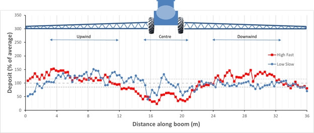
A third issue to consider is less related to boom height but nonetheless affects spray distribution. Small droplets move with air currents, and the turbulence created by large, fast sprayers creates enough turbulence to move these droplets significantly. A perfect pattern under static conditions can look quite different at a fast travel speed with a modest side wind. Low booms may help prevent some of this displacement because droplets spend less time in flight, and their average velocity is faster.
Figure 7: Spray deposition onto a 2 mm string to measure deposit uniformity for a fast travel speed and high boom and a slow speed, low boom configuration.
Flow Rate Math
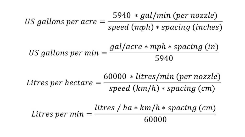
Flow rate requirements per nozzle change whenever we equip a boom at an alternate spacing. The basic formulae are shown below.
Moving from a 20″ to a 15″ spacing would require a nozzle with 0.75 of the flow rate, approximately from a 02 to 015 size, or 03 to a 025 size, or 04 to 03 size, etc.
Pulse Width Modulation
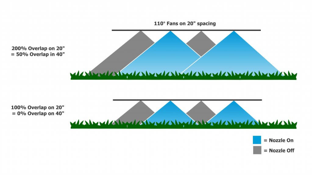
The use of Pulse Width Modulation (PWM) has increased the overlap requirement. With PWM, alternate nozzles are on a 180° timing offset from their neighbours. This means that when running >50% duty cycle, when one nozzle is temporarily off, its neighbours are on. These neighbours’ patterns must now span the gap, and 100% overlap is the absolute minimum to achieve this. PWM users therefore select the wider pattern angles and some opt for >100% overlap.
Figure 8: Pulse Width Modulated booms require 200% overlap so that the entire boom receives proper coverage when the alternate set of nozzles is off. For 110° fans at 20″ spacing, the minimum boom height would be 21″
PWM Considerations
High flows (greater than 1 US gpm at the nozzle) that are common for fertilizer top-dressing may require higher-flow PWM valves.
Narrow spacings reduce the individual nozzle flow rates and can therefore support higher application rates before triggering a larger valve requirement.
PWM valves aren’t cheap and for example 15″ spacing compared to 20″ spacing adds 24 valves on a 120′ boom.
Banding
We noted that 20” nozzle spacing is a standard because it corresponds to what has traditionally been achievable with available boom heights and spray pattern angles. But things can change.
Narrower spacings such as 15” originate with row crops and planter row spacings of 15” or 30”. These spacings exist so the spray pattern can be placed either over the top of a crop row, or in between the rows for banding. Using narrower fan angles and/or lower boom heights, together with “even” (as opposed to “tapered”) fans, banding sprays can be applied over the top of, or between crop rows. Or drop hoses can reach between the rows for top-dressing or directed sprays into the canopy.
Canopy Penetration
With narrower spacing, it can be argued that a greater proportion of the boom length has spray directed directly downward (corresponding to the centre of the pattern). Whether or not this translates into better penetration of a canopy is a fair question. In laboratory trials, use of 10” or 20” spacing did not improve penetration into a broadleaf canopy. But if the lower boom height afforded by the narrower spacing was utilized, some improvements in the deposit of angled sprays onto vertical targets was observed.
Adjusting to Narrower Spacings
As we showed earlier, use of 15” or 10” spacing booms for broadcast sprays requires a smaller nozzle size to achieve the same spray volumes as the 20” spacing. If boom height remains constant, narrower spacings result in greater pattern overlap which provides more latitude for sway. Alternately, lower boom heights can be used.
Using smaller nozzles on narrower spacing presents some challenges. Generally, smaller nozzle size means finer spray quality. If an operator wants to retain the spray quality they had on a 20″ spacing, they may opt to use lower pressure (not advisable for non-PWM systems) or swap to different nozzle design that can produce the desired spray quality at the lower flow rate.
Smaller nozzles are more prone to plugging, so that needs to be managed with filtration, filling practices and water sourcing. Be aware of the the product formulations and their requirements for filter mesh size. Most dry products specify a 50 mesh filter (or coarser). Also, check size options for nozzles. The smallest size for most nozzle models is 015, but certain PWM-specific nozzles are only available in 03 or larger.
The marriage of narrow spacings with individual nozzle shutoff can result in a versatile system capable of producing high resolution banded sprays in narrow seeded crops. For example, consider a boom with a 10” nozzle spacing spacing that matches the seeder row spacing. The operator can shift from 10” to 20” or 30” from the cab if the valve control software allows it. With accurate guidance and good boom levelling, topdressing foliar products (e.g. nutrients, fungicides) can follow the crop row precisely.
Spot Sprays
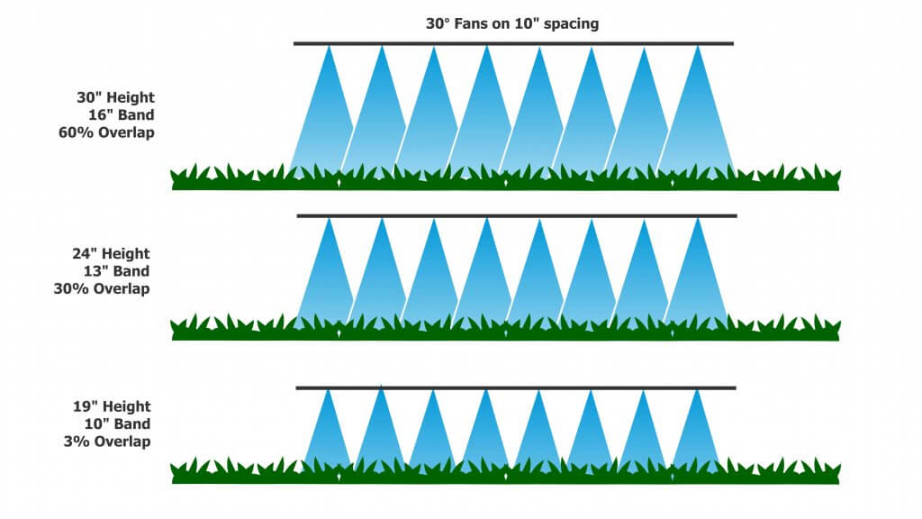
Spot sprays present a situation where compromises are needed. Some, such as WEEDit, utilize narrower nozzle spacings to allow better treatment resolution and increase product savings. Any one nozzle or sets of adjacent nozzles may be triggered by the sensor. For single nozzle activation, to preserve the value of the better resolution a uniform, narrow band of spray needs to be created. This means a 30° or 40° fan angle from a banding nozzle will be necessary. For example, a 24” boom height will result in a 13” band with a 30° fan, and an 18” band with a 40° fan. In the latter case, the dose would be diluted by 80%, wasting much of the potential savings.
Figure 10: Boom height is critical for banded sprays and for spot sprays. Too wide a pattern on a single nozzle reduces dose, too narrow creates misses.
Frequently, a patch of weeds will trigger several adjacent nozzles. Now these individual bands need to work together to create a uniform swath. This will inevitably require some overlap to avoid gaps, but too much overlap will result in bands where twice the dose will be applied. A tapered fan may suit this situation better. As a result of these varying needs, tolerances for spot spray boom height are even more strict than for broadcast spraying. More thoughts on spot spray nozzle selection are here.
Conclusions
Narrower nozzle spacings on a broadcast boom allow somewhat lower boom heights and these can in turn reduce drift and improve deposition of sprays. Lower flow nozzles will be needed with narrower spacings, requiring management of plugging and potentially a more drift-prone spray quality. The value of narrower spacings depends on the availability of booms that control sway, allowing them to operate at uniform, low heights.
Download the 2023 publication from Crop Protection here.
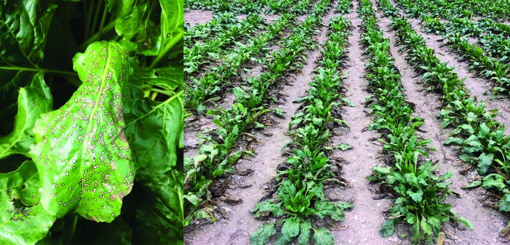
Cercospora leaf spot (CLS), caused by the fungal pathogen Cercospora beticola, is one of the most damaging foliar diseases affecting sugarbeet (Figure 1) (Khan et al. 2008). Growers rely on broad-spectrum contact fungicides because they are less likely to cause fungicide resistance (OMAFRA 2020). However, these fungicides are usually less effective than other fungicides (Trueman & Burlakoti 2014), and require frequent reapplications (Thind & Hollomon 2018) and good coverage to be effective (Prokop & Veverka 2006; Roehrig et al. 2018).
Figure 1. Cercospora leaf spot on sugarbeet.
We evaluated practices intended to improve the efficacy of Manzate® Pro-Stick™ (Mancozeb) by improving deposition and penetration into the sugarbeet canopy. Practices included different nozzle types (Shepard et al. 2006; Dorr et al. 2013), carrier volumes (Armstrong-Cho et al. 2008; Roehrig et al. 2018; Tedford et al. 2018) and the addition of InterLock®. InterLock is a spray adjuvant made with modified vegetable oil (MVO), vegetable oil and a polyoxyethylene sorbitan fatty acid ester emulsifier. It is intended to reduce the number of drift-prone, fine droplets without compromising the volume median diameter (WinField® 2019).
Research
In 2019 and 2020, InterLock and carrier volume were assessed to evaluate effects of:
InterLock on Manzate Pro-Stick efficacy at different carrier volumes.
InterLock on spray deposition and penetration within the sugarbeet canopy.
Objective 1: InterLock on Manzate Pro-Stick efficacy at different carrier volumes
Four replicated field trials were conducted at two sites, Dealtown (2019) and Ridgetown (2019 and 2020). Treatments were evaluated using four carrier volumes: 115, 235, 350, and 470 L ha-1 (12, 25, 37, and 50 gpa) and applied on a 14-day schedule.
Results
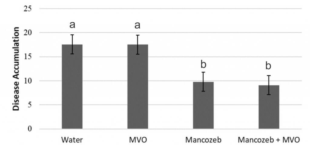
Adding InterLock to Manzate Pro-Stick did not reduce disease accumulation over the season (Figure 2a) or improve beet and sugar yield or sugar quality compared to applications of Manzate Pro-Stick alone (data not shown).
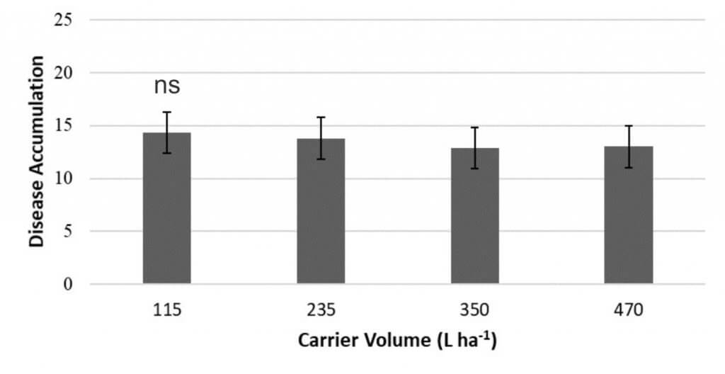
Carrier volume did not affect disease accumulation (Figure 2b).
Figure 2a. Disease accumulation (standardized area under the disease progress stairs; sAUDPS) (±SE) for fungicide treatments applied to sugarbeets in Ridgetown and Dealtown ON 2019, and in Ridgetown 2020. Bars followed by the same letter are not significantly different at p ≤ 0.05, Tukey’s HSD, ns= not significant.Figure 2b. Disease accumulation (standardized area under the disease progress stairs; sAUDPS) (±SE) for carrier volume applied to sugarbeets in Ridgetown and Dealtown ON 2019, and in Ridgetown 2020. Bars followed by the same letter are not significantly different at p ≤ 0.05, Tukey’s HSD, ns= not significant.
Objective 2: InterLock on spray deposition and penetration within the sugarbeet canopy
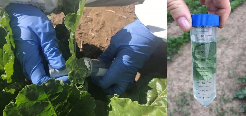
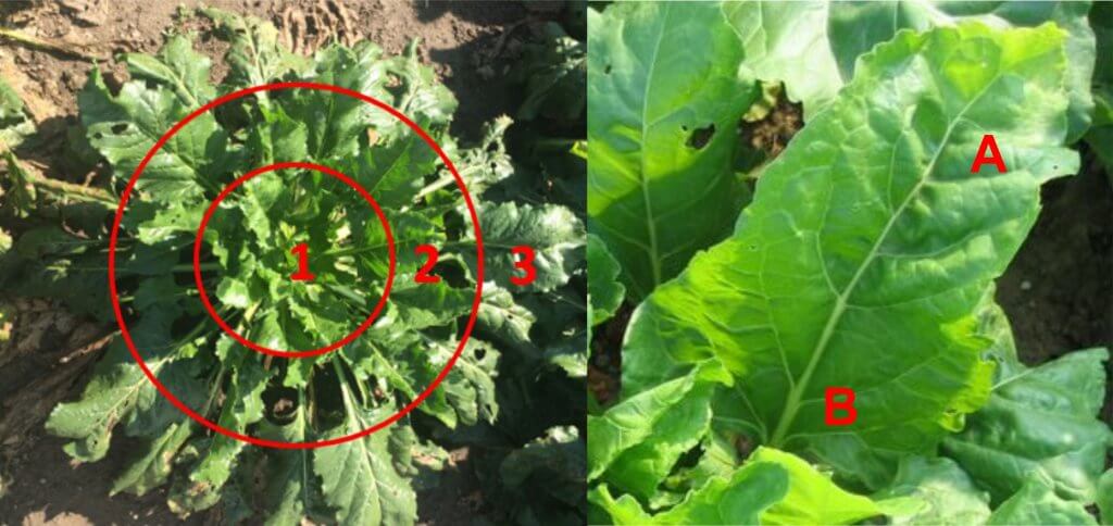
Deposition was evaluated using Rhodamine WT dye recovery. The amount of dye recovered for a treatment (µL AI/ g leaf tissue) was used to make assumptions about treatment deposition in the sugarbeet canopy. To assess spray deposition, samples were taken from six canopy locations (Figure 3 and 4).
Figure 3. Leaf sample collection from sugarbeet canopy.Figure 4. Leaf samples were taken from a) three canopy locations 1= inner, 2= mid, 3= outer from b) two leaf locations each A= tip, B= base.
Three sets of replicated experiments were conducted in Ridgetown (2019 and 2020) to evaluate the effect of InterLock on canopy deposition when 1) mixed with Manzate Pro-Stick, 2) using three different nozzle types, and 3) using three carrier volumes.
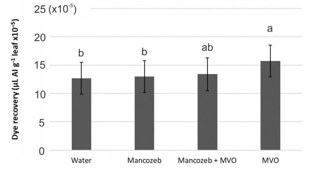
In the first study, four programs (Manzate Pro-Stick + InterLock, Manzate Pro-Stick alone, InterLock alone, and water) were evaluated for dye recovery.
Results
Deposition was improved for the InterLock only treatment compared with water, but when InterLock was applied with Manzate Pro-Stick the deposition was the same as Manzate Pro-Stick applied alone (Figure 5). It is possible that the fungicide formulation or active ingredient had an antagonistic effect with InterLock, though we cannot determine that from this study.
Figure 5. Effect of program on mean Rhodamine WT active ingredient (µL per gram of dry leaf) (±SE) recovered from six locations in a sugarbeet canopy at the 13 (Trial 1) and 16 (Trial 2) leaf stage in Ridgetown, ON 2019. Bars followed by the same letter are not significantly different at p ≤ 0.05, Tukey’s HSD.
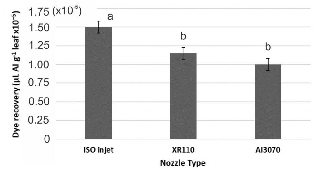
In the second study Manzate Pro-Stick + InterLock and Manzate Pro-Stick were applied using three different nozzle types at ~40 psi:
The Hardi ISO Injet is an air inclusion 110° flat fan that produces a Very Coarse spray quality.
The TeeJet XR110 is a conventional 110° flat fan that produces a Medium spray quality.
The TeeJet AI3070 is an air inclusion, dual flat fan (30° and 70° spray angles) that produces a Coarse spray quality.
Results
Adding InterLock did not affect deposition and did not alter the performance of any nozzle type (data not shown).
Deposition among nozzles did differ, with the ISO injet nozzle providing improved deposition compared to the XR110 and AI3070 nozzles (Figure 6).
Figure 6. Effect of nozzle type on mean Rhodamine WT active ingredient (µL per gram of dry leaf) (±SE) recovered from six locations in a sugarbeet canopy at the 15 (Trial 3), 18 (Trial 4), and 19-22 (Trial 5) leaf stage in Ridgetown, ON 2019 and 2020. Bars followed by the same letter are not significantly different at p ≤ 0.05, Tukey’s HSD.
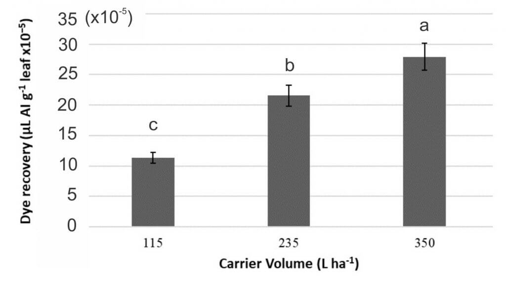
In the third study, Manzate Pro-Stick + InterLock and Manzate Pro-Stick were applied using three carrier volumes: 115, 235, and 350 L ha-1.
Results
The addition of InterLock had no effect on deposition, regardless of carrier volume (data not shown).
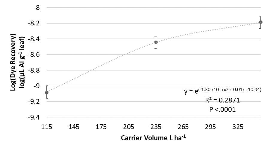
Deposition increased with increasing carrier volume (Figure 7a). A regression analysis determined a curvilinear relationship between carrier volume and deposition, predicting that deposition would increase with increased carrier volume until a maximum carrier volume was reached (Figure 7b). Many studies indicate that at exceptionally high carrier volumes coverage can be reduced primarily due to run-off.
Even though increased carrier volume improved fungicide deposition, increased volume did not improve fungicide efficacy for CLS management (Objective 1 efficacy trials).
Figure 7a. Effect of carrier volume on mean Rhodamine WT active ingredient (µL per gram of dry leaf) (±SE) recovered from six locations in a sugarbeet canopy at the 20 and 23 leaf stage in Ridgetown, ON 2020 (Trial 6 & 7). Bars followed by the same letter are not significantly different at p ≤ 0.05, Tukey’s HSD.Figure 7b. Regression of carrier volume (115, 235, 350 L ha-1) and mean Rhodamine WT active ingredient (±SE) recovered from six locations in a sugarbeet canopy at the 20 and 23 leaf stage in Ridgetown, ON 2020 (Trial 6 & 7). Data analysis was performed on the log normal scale, means and SE presented have not been back-transformed.”
Canopy location was an important factor in all experiments
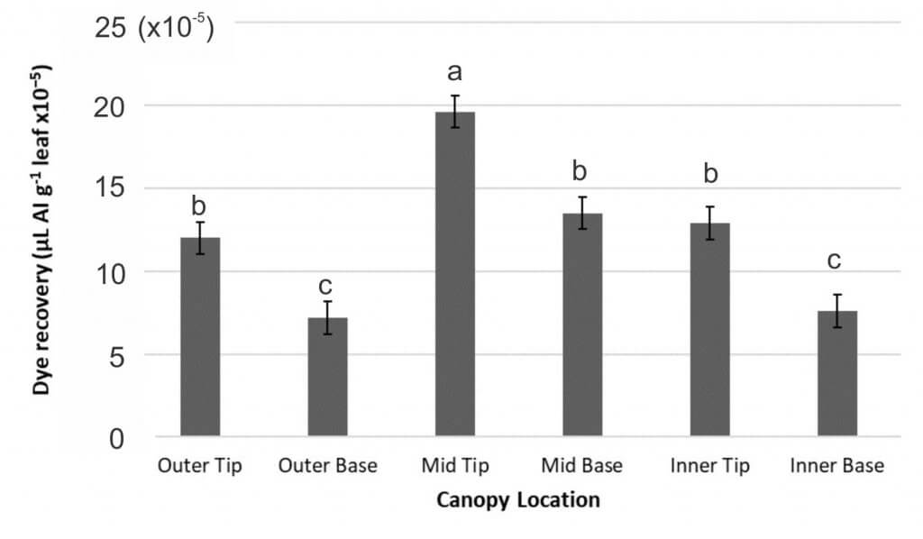
The least deposition was always found in the outer and inner canopy from the base of the leaf, and in the outer canopy from the tip of the leaf (Figure 4), suggesting that these locations are the most challenging to achieve spray deposition. An example from the nozzle type experiment is shown in Figure 8. One of the proposed benefits of InterLock is for improved spray penetration, but in the current study, InterLock did not improve penetration of Manzate Pro-Stick into any of the harder to reach canopy locations.
Figure 8. Effect of canopy location on mean Rhodamine WT active ingredient (µL per gram of dry leaf) (±SE) recovered from six locations in a sugarbeet canopy treated with InterLock and different nozzle types at the 15-22 leaf stage in Ridgetown, ON, 2019 and 2020 (Trials 3, 4 & 5). Bars followed by the same letter are not significantly different at p ≤ 0.05, Tukey’s HSD.
Conclusion
Adding InterLock to Manzate Pro-Stick did not improve deposition in any field experiment regardless of the nozzle type or carrier volume used. Further, using InterLock with Manzate Pro-Stick did not improve fungicide efficacy for CLS management. However, we cannot determine from this study if InterLock would improve deposition, penetration, or fungicide efficacy using other fungicide products.
Despite findings of improved disease management with the use of larger carrier volume, fungicides are sometimes still applied with smaller carrier volumes of 100 L ha-1 or less (Armstrong-Cho et al. 2008; Roehrig et al. 2018) to save time and reduce the cost of application. In this experiment, increased carrier volume improved deposition but did not improve fungicide efficacy of Manzate Pro-Stick for CLS management. There is the potential that using increased carrier volume may be more beneficial in years with a greater disease severity, and may thus be worthwhile to growers, as has been observed in previous research on Cercospora leaf spot in Ontario (Tedford et al. 2018).
This research was sponsored from the Canadian Agricultural Partnership, Ontario Agri-Food Innovation Alliance, Ontario Sugarbeet Growers’s Association, and the Michigan Sugar Company.
References
Armstrong-Cho C, Wolf T, Chongo G, Gan Y, Hogg T, Lafond G, Johnson E, and Banniza S. 2008. The effect of carrier volume on Ascochyta blight (Ascochyta rabiei) control in chickpea. Crop Prot. 27: 1020-1030.
Dorr GJ, Hewitt AJ, Adkins SW, Hanan J, Zhang H, and Noller B. 2013. A comparison of initial spray characteristics produced by agricultural nozzles. Crop Prot. 53: 109-117.
Khan J, del Rio LE, Nelson R, Rivera-Varas V, Secor GA, and Khan MFR. 2008. Survival, dispersal, and primary infection site for Cercospora beticola in sugar beet. Plant Dis. 92: 741-745.
Ontario Ministry of Agriculture, Food, and Rural Affairs (OMAFRA). 2020. Vegetable Crop Protection Guide, Pub 838. Sugarbeets. Queen’s Printer for Ontario, Toronto.
Prokop M, and Veverka K. 2006. Influence of droplet spectra on the efficiency of contact fungicides and mixtures of contact and systemic fungicides. Plant Protect. Sci. 42: 26-33.
Roehrig R, Boller W, Forcelini CA, and Chechi A. 2018. Use of surfactant with different volumes of fungicide application in soybean culture. Eng. Agr. Jaboticabal 38: 577-589.
Shepard D, Agnew M, Fidanza M, Kaminski J, and Dant L. 2006. Selecting nozzles for fungicide spray applications. Golf Course Manag. 74: 83-88.
Tedford SL, Burlakoti RR, Schaafsma AW, and Trueman CL. 2018. Optimizing management of Cercospora leaf spot (Cercospora beticola) of sugarbeet in the wake of fungicide resistance. Can. J. Plant Pathol. 41: 35-46.
Thind TS, and Hollomon DW. 2018. Thiocarbamate fungicides: Reliable tools in resistance management and future outlook. Pest Manag. Sci. 74: 1547-1551.
Trueman CL, and Burlakoti RR. 2014. Evaluation of products for management of Cercospora leaf spot in sugarbeet, 2014. Plant Disease Management Reports. 9: FC009.
WinField United. 2019. InterLock. [Internet]. [cited 2019 Feb 25].
In June 2013 we ran a ginseng spraying workshop and we learned as much as the growers did. Ginseng is notoriously difficult to spray:
It is highly susceptible to pathogens given the high humidity and still conditions generally found under the shade structure.
It forms a solid ceiling of leaves that resist spray penetrating to the stem and crown below and makes under-leaf coverage very difficult to achieve.
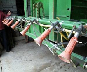
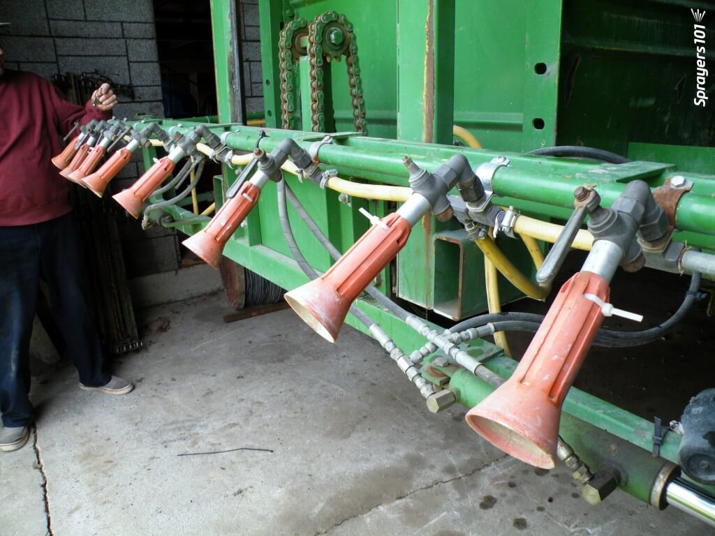
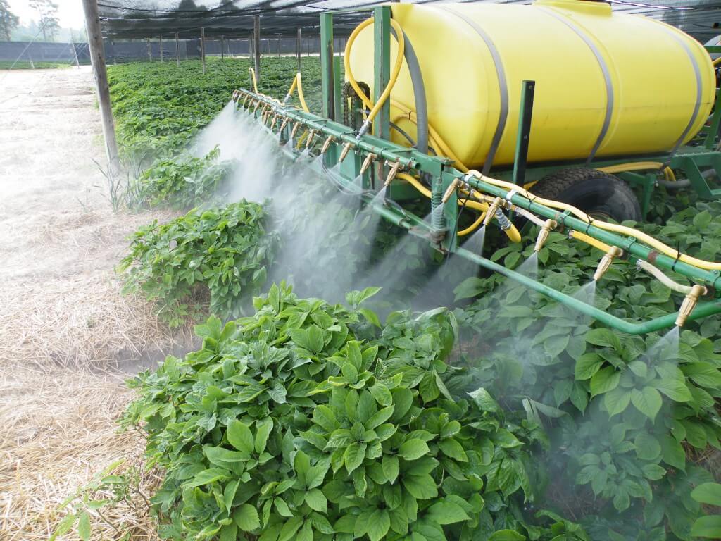
Many growers have (wisely) walked away from the old Casotti sprayers, which have been shown to give erratic coverage at best. They have adopted the Arag Microjet system with it’s characteristic orange shields. The >$80.00 CAD price tag for each nozzle is due to the brass mixing valve and swivel joint, as well as import costs from Italy. Contrary to popular belief, it does not use air-assist, or air-induction – it is strictly hydraulic. It does tend to create a ‘wake’ of air movement at high pressure. This phenomenon is called air entrainment and it is caused by large droplets travelling at high speed.
Classic Arag microjet nozzles.
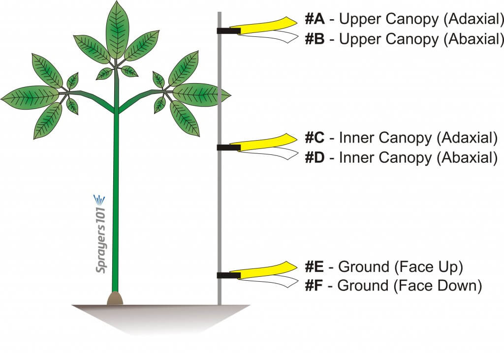
This nozzle is essentially the business-end of a spray gun. The way it is used in ginseng it works more-or-less like a hollow cone disc-core assembly. This begs the question “Why not use the cheaper and more readily available ceramic disc-core?” We set out to compare the two options using water sensitive paper set within the canopy. These yellow, paper targets turn blue when sprayed, clearly showing spray coverage.
Location of water sensitive papers in the ginseng canopy.
Determining rates
The first step was to determine the output rate for each nozzle. Generally, nozzle manufacturers provide rate tables showing how much volume a nozzle emits by time (e.g. US gallons per minute) at a given pressure. Finding these tables for the 1.5 millimetre Arag Microjet proved difficult. When we finally found one, it was discovered the rates were established for 200 to 850 pounds per square inch. This is excessively high pressure for a typical boom sprayer, so tables had to be developed for lower pressures.
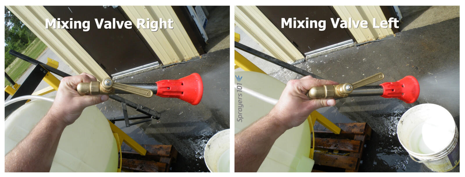
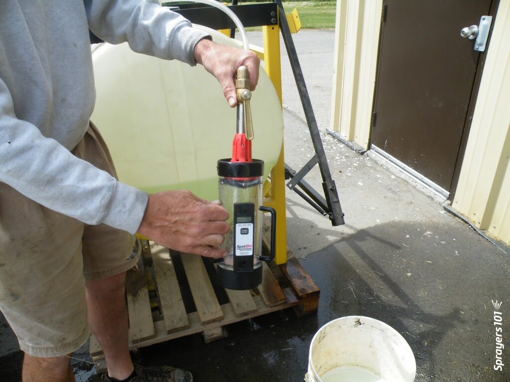
Classic Arag microjets have a mixing valve that opens the spray up into a hollow cone (valve handle left or right), or collapses it into a tight stream (valve handle middle). The valve position also changes the rate. It can never be shut off completely, and it’s hard to adjust consistently.Determining nozzle rate using the Innoquest Spot-On SC-4.
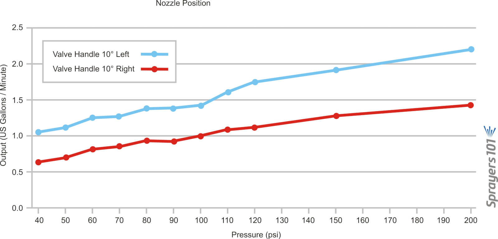
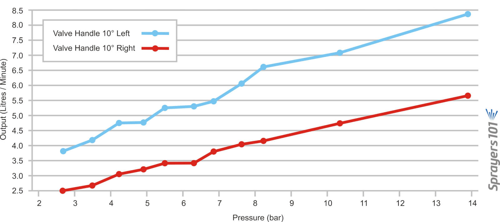
Further, given the odd design of the mixing valve, it was determined that moving the handle ~10 degrees left of centre, or ~10 degrees right of centre, gave a difference of as much as 60%. The table below shows the outputs for a 1.5 millimetre nozzle with the handle in both positions and the two graphs show the results… well… graphically. Outputs were determined using the Innoquest Spot-On SC-4, but the frothing effect created by the nozzles may have created minor errors. Each rate is the average of a minimum of three samples.
Valve Setting
Pressure (psi)
Avg Output (gpm)
Pressure (bar)
Avg Output (L/min)
10 degrees left
40
1.02
2.76
3.86
10 degrees left
50
1.1
3.45
4.16
10 degrees left
60
1.25
4.14
4.73
10 degrees left
70
1.25
4.83
4.73
10 degrees left
80
1.38
5.52
5.22
10 degrees left
90
1.4
6.21
5.3
10 degrees left
100
1.45
6.89
5.49
10 degrees left
110
1.6
7.58
6.06
10 degrees left
120
1.75
8.27
6.62
10 degrees left
150
1.87
10.34
7.08
10 degrees left
200
2.2
13.79
8.33
10 degrees right
40
0.65
2.76
2.46
10 degrees right
50
0.7
3.45
2.65
10 degrees right
60
0.8
4.14
3.03
10 degrees right
70
0.85
4.83
3.22
10 degrees right
80
0.9
5.52
3.41
10 degrees right
90
0.9
6.21
3.41
10 degrees right
100
1
6.89
3.79
10 degrees right
110
1.07
7.58
4.05
10 degrees right
120
1.1
8.27
4.16
10 degrees right
150
1.25
10.34
4.73
10 degrees right
200
1.37
13.79
5.19
Average 1.5 mm ARAG Microjet output at a range of pressures and two valve settings in US Imperial units.Average 1.5 mm ARAG Microjet output at a range of pressures and two valve settings in Metric units.
Comparing nozzles
Using the grower’s typical ground speed of 5 km/h (~3 mph) and operating pressure of 6.9 bar (100 psi), we found four TeeJet disc-core combinations that emitted a hollow cone pattern and approximately the same output as the Arag Microjets. The five nozzles sets tested were:
ARAG Microjet® 1.5 mm = ~0.95 US g/min avg at 100 psi
TeeJet® D8-DC25= 0.97 US g/min at 100 psi= ~97° cone
TeeJet®D7-DC45= 0.97 US g/min at 100 psi= ~81° cone
TeeJet®D4-DC46= 0.88 US g/min at 100 psi= ~33° cone
TeeJet®D6-DC45= 0.93 US g/min at 100 psi= ~81° cone
We did not use nozzle drop hoses (aka drop arms or hose drops) because it has already been firmly established that they are absolutely required to achieve under leaf coverage See OMAFRA factsheet 10-079 and this article.
Observations
While there were some complications with setting up the papers for the demo, we observed the following:
The output of each Microjet nozzle can be as much as 50% more or less than expected without being visually detectable and output for each nozzle must be confirmed before spraying. Therefore, outputs should be confirmed before every application.
Microjets at 100 psi emitting ~890 L/ha (~95 US gallons per acre) gave satisfactory coverage on all upward facing targets, but unsatisfactory under-leaf coverage. This has been demonstrated many times before.
The TeeJet D7-DC45 combination emitting a similar rate gave satisfactory coverage on all upward facing targets, but unsatisfactory under-leaf coverage. They may be a viable alternative to the Microjets.
Nozzle drops are advised to achieve under-leaf coverage.
The demo also raised some questions:
Did the TeeJet disc-core push the canopy apart as much as the Microjet? The audience noticed there was some leaf-shadowing where the cards did not get complete coverage using disc-core. This might have been coincidence, or it may not have. This question will be addressed in a research trial next season, but for now, the D7-DC45 appeared to give similar coverage to the Microjet.
Can nozzle drops be avoided if pressure is raised to 27.5 bar (400 psi)? Thanks to one grower trying this experiment in his garden after the demo, we saw some under-leaf coverage is possible at such high pressures, but this occurred at the cost of a lot of noise, diesel fuel and considerable wear on the ceramic Microjet discs. The grower tested these tips and discovered they needed replacement after only two years of use. Nozzle drops are cheaper, easier and result in considerably more spray in the under leaf positions.
We saw what minimal and excessive foliar coverage looked like, and determined how much variability there was from one nozzle to another. A significant question was “How much spray can be saved when using a more accurate application?” and the answer is yet to be determined, but could be well in excess of 10% of the typical spray volume. Given that this crop can be sprayed more than 100 times over it’s 3 or four years before harvest, this represents significant savings in pesticides and refill time.
Additional – Newer ARAG Microjet Design
Since this work was performed, growers have been exploring a newer option from ARAG.
They are an improvement over the older version insofar as they are more easily calibrated and held at a given rate thanks to a lock nut. They still employ a 1.5 mm diameter ceramic disc, but this can be changed for a 1.0 or 1.2 quite easily. They are still somewhat finicky when trying to set a consistent spray quality and rate from nozzle to nozzle, but are better than the mixing-valve option.
Custom-made ginseng sprayer. A standard design with newer, cheaper and easier-to-use ARAG microjets.
Special thanks to Syngenta Canada for providing lunch, to C&R Atkinson Farms Ltd. for hosting, to TeeJet for supplying the disc-cores and water-sensitive papers, and to Dr. Sean Westerveld, Dr. Melanie Filotas and OMAFRA summer student Megan Leedham for contributing to the workshop.
This is the final part of our three-part article discussing methods for digitizing and processing water sensitive paper. You can read part one here and part two here.
Morphological operations
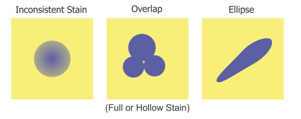
We can now move on to the larger shapes, or “morphology” of the objects in our binary image. Our goal is to quantify deposits by interpreting these shapes. Once again, these operations are powerful processing tools, but we must acknowledge three overriding limitations:
1. Inconsistent stains
Sometimes deposits do not create a consistent blue colour – they can get lighter or take on a greenish-yellow hue towards the perimeter of the stain. During thresholding, the outer edge can be accidently eroded, leaving behind an object with a jagged edge. This may lead us to underestimate the percent area actually covered. In the case of tiny stains, it might eliminate them entirely and lead us to underestimate deposit density.
2. Overlaps
It can be difficult to determine if an object represents a stain from a single droplet or is the result of multiple, overlapping deposits. This becomes significant when the surface of the WSP exceeds ~20% total coverage. The resulting objects may or may not have hollow centres where droplets do not overlap entirely. Misidentifying overlaps leads us to falsely conclude that an object is the result of a single, coarser droplet rather than multiple finer droplets.
3. Ellipses
Non-circular stains are formed when droplets scuff along the surface. Two droplets with the same volume encountering a paper at different angles can create stains with significantly different areas. We may wrongly conclude that the droplets that created them were coarser than they truly were. One approach is to use Feret’s Diameter (aka Caliper Diameter) by measuring the widest spans on the X and Y axes and taking the average. Another approach is to interpret the ellipse as a series of circular stains. Or we can decide to only acknowledge these objects when calculating percent area covered, but omit them when calculating deposit density or predicting original droplet size. Each strategy is a compromise, so it is important to be consistent and transparent when reporting results.
Three common problems when analysing water sensitive paper.
We’ll explore two morphological operations that can help us separate fact from fiction: Granulometry and Dilation-and-Erosion. We’re introducing these operations as part of the processing and detection step, but they may also overlap with the measurement step in our three-step process.
Granulometry
We can estimate the range of object sizes and get a sense of how they are distributed on the paper by filtering or “sieving” the image. Imagine pouring a mixture of sand and rocks through a series of ever-finer sieves. Doing so allows you to separate particles based on size exclusion. A granulometry function compares each object to a series of standardized objects with decreasing diameters. This isolates objects of a similar size and bins them in that size range. This is a powerful operation, but accuracy is lost when stains overlap to form larger objects. In this case, we move on to Dilation and Erosion.
Dilation and Erosion
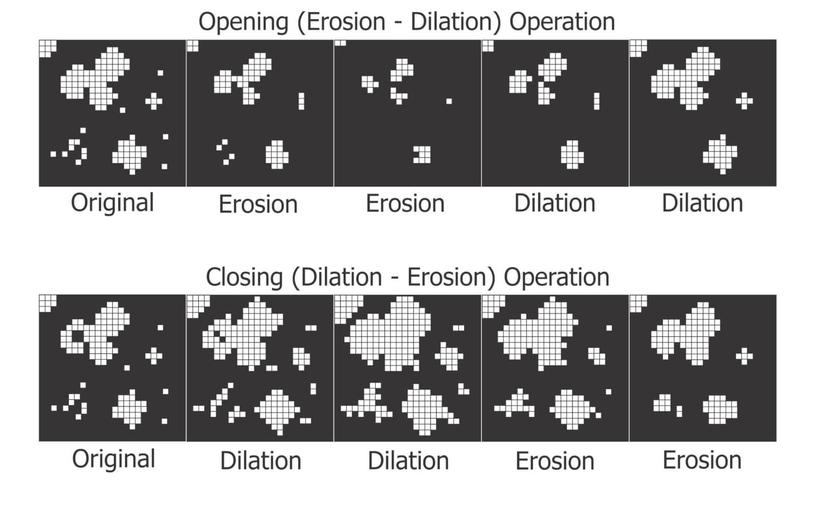
Think of dilation as adding pixels to the boundary of an object. This makes tiny objects bigger, fills in any interior holes and can cause objects to merge. The number of pixel-wide dilations required to make objects contact one another can be used as a measure of deposit density.
Erosion removes pixels from the outer (and sometimes inner) boundaries of an object. This eliminates tiny artifacts that may not actually represent stains. It can also split non-circular objects into multiple parts before shrinking them into multiple nuclei (aka centroids). These last-remaining points are not necessarily the centre of a stain, but the pixels furthest away from the original boundary.
When a non-circular shape has more than one nucleus, they likely represent individual droplets that combined to form the larger stain. We can then use these nuclei to measure deposit density, such as in a Voronoi partition which triangulates each nucleus in relation to the two closest neighbours.
Many image processers use both these operations sequentially. When an image is eroded and then dilated (a process called “Opening”), smaller objects are removed, leaving the area and shape of remaining objects relatively intact. Dilating and then eroding (a process called “Closing”) fills in small holes and merges smaller objects, once again leaving the area and shape of remaining objects relatively intact. We can use both of these functions to help smooth an image prior to measurement.
(Top) Opening operations erode and then dilate the image. Moving left to right, the smaller objects tend to disappear. (Bottom) Closing operations dilate and then erode the image. Moving left to right, smaller objects either disappear or merge and holes are filled in
Distance Transformations
Distance transformations are advanced operations specifically used to separate objects that are densely packed. While not typically used when analyzing WSP, distance transformations are another means of identifying object nuclei. They are another means for teasing apart objects that are likely the result of overlapping deposits and then mapping their relative sizes and positions.
Measurement
The calculation of the area covered by deposits is straightforward. The pixels belonging to objects (the deposits) and those belonging to background are summed and then the fraction is converted to percent area covered. Research has shown that the image resolution does not significantly impact percent coverage assessments and has suggested that all image analysis software tends to produce similar results (+/- 3.5% observed when the same threshold was applied to multiple papers). This is acceptable because it’s within the variability inherent to spraying.
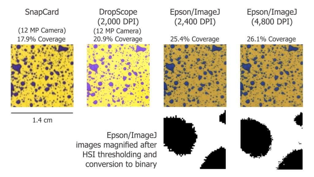
We ran a similar experiment wherein we analyzed the same piece of WSP using four methods. Here are a few facts about the software we used:
DropScope produces images between 2,100 and 2,300 DPI. Currently, it ignores ellipses and doesn’t count anything spanning less than ~35 µm (3 pixels).
We set ImageJ to ignore any object spanning less than 3 pixels, which at 2,400 DPI was 30 µm in diameter.
Snapcard was a free app created by Australia’s GRDC. It was benchmarked using ImageJ, tended to underestimate coverage and was fairly inconsistent. Nevertheless, it was convenient for field work. Instances may still exist, but as of 2025 it no longer available through the GRDC.
The images shown in the figure below were cropped from screenshots produced by each method. The actual ROI analyzed was ~3 cm2 for SnapCard, 3.68 cm2 for DropScope and 2.0 cm2 for both Epson/ImageJ methods. Our results indicate an +/- 4% difference in percent area coverage. This variability reflects the results of a 2016 journal article that compared SnapCard with ImageJ and other leading analytical software. That study claimed no statistically significant difference in percent coverage detected (standard deviations were about 20%). However, the ImageJ results tended to trend several percent higher than SnapCard. We saw this as well. And so, while resolution may not have a significant impact on percent area covered, there does appear to be some correlation.
Percent area covered as reported by three image analysis systems. Only a minor difference was observed when resolution was doubled using the Epson/ImageJ method.
Resolution definitely affects deposit counts. Particularly in applications that employ finer droplets. Consider the difference between detecting or missing 1,000 30 µm diameter objects. It may only amount to a fraction of a percentage of the surface covered, but +/- 1,000 objects on a 2 cm2 area is significant in terms of deposit density.
Output
Once a WSP image (or set of images) has been scanned, pre-processed, processed and measured, we will receive some manner of output. Some software packages create an attractive report with images, graphs and key values. These reports include percent coverage and many provide droplet density. Deposits may be binned by size, or spread factors are used to calculate the original droplet diameters and even estimate the volume applied by area. Other software packages provide raw data that can be imported into a statistical program or spreadsheet program like Excel for further analysis. Some software packages provide both.
How far can we take this?
Blow-by-blow data analysis is beyond the scope of this document, but how much weight should we give to coverage data obtained using WSP? The answer depends on the metric in question, but in all cases we must first acknowledge the three overriding caveats. Take it as said that they apply to everything that follows:
Different brands (and even different production runs) of WSP can produce significantly different coverage metrics. When conducting experiments, use a single brand of WSP. Better still, use papers from the same production batch whenever possible.
The same of piece of sprayed WSP can produce significantly different results depending on the software and protocol used to analyze it. When conducting experiments, use the same software and assessment protocol and be transparent about the process when communicating results.
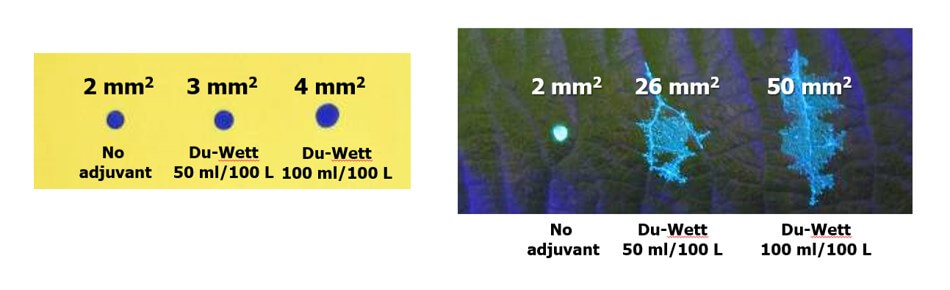
WSP coverage may not reflect the coverage achieved on an actual plant tissue surface. It is suitable as a relative index (I.e. papers can be compared to papers, but not to tissues) but the spread factor changes with surface wettability and the surface tension of the liquid sprayed. Note the differences in percent area covered in the following experiment with an organosilicone super-spreader:
Difference in deposit spread on water sensitive paper versus a leaf surface using an organosilicone super-spreader and UV dye. The same volume was applied in each case and while the area increased two-fold on WSP it increased ~10-fold on an actual leaf. Image reproduced from work by Robyn Gaskin, Plant Protection Products, New Zealand.
Recall that we started this document by listing the four pieces of information commonly sought using WSP. They were listed in order of reliability, and now we can explain why.
The percent surface area covered: We have established that this is the most reliable piece of data. Droplets do not spread on WSP the way they do on plant surfaces, so it will underestimate actual coverage. The results vary by analytical method, but it’s likely not dependent on resolution and still falls within the variability inherent to spraying. This metric gives us valuable and actionable information. We can say whether or not we hit a target, and evaluate whether a sprayer change resulted in more or less deposit.
The density of deposits on the target area: We have established that that there are limits to the reliability of this metric. It is affected by the analytical method used and can be greatly underestimated when resolution is poor or when deposits overlap in high numbers. Also, it will never reliably reflect deposits under 30 µm. Nevertheless, under controlled conditions this information does have value and is of great interest in enquiries about drift and contact fungicides.
The size of the droplets that left the stains: This metric is highly questionable except under controlled conditions. The many assumptions about surface tension, droplet speed, and droplet evaporation make it impossible to make definitive statements about spray quality. Finer droplets are greatly underestimated in this equation. Therefore, while there may be some value in using WSP as a relative index, this metric is a crude indication at best.
The dose applied to the target surface: This metric has not been discussed up to this point, but is quickly and easily dismissed. Let’s assume that a droplet with a high concentration of an active ingredient will leave a stain that is the same area as another droplet with a lower concentration. This will lead some to suggest that as long as the original concentration is known, we can back-calculate the dose (which is the amount of active on a given area). However, one droplet has the same volume as eight droplets that are half it’s diameter. This cubic relationship means that if they all deposit, the larger droplet will cover roughly 1/2 the surface area as the eight smaller droplets. Therefore, the smaller droplets spread the same amount of active over a greater area. Spread factor muddies this a bit, but ultimately it means that dose cannot be estimated from area covered. Dose is better assessed using collectors that permit the residue to be removed, such as Petri dishes, Mylar sheets, pipe cleaners, alpha cellulose cards, or glass slides.
And so, the image analysis process described here is powerful and effective when used with water sensitive paper as long as the limitations are acknowledged. The same process can also be used with dyes and specialized collectors such as Kromekote to permit even greater resolution. But that’s another story.
2026
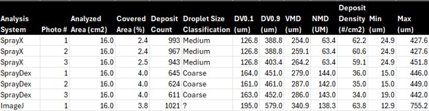
A new Brazilian cellphone-based system (SprayDex) emerged in 2026 that offers possibilities. Preliminary testing alongside other methods indicate it is consistent within itself, but as we saw in previous testing, the same WSP scanned using different systems will create different results. This is why, ultimately, WSP is a relative index and should only be compared within a given system; coverage cannot be reliably compared across WSP brands, or between digitization methods.
2026 Comparison of three digitization / analysis methods. Same WSP was scanned each time.
Marçal, A.R.S., Cunha, M. 2008. Image processing of artificial targets for automatic evaluation of spray targets. Trans. of the ASABE. 51(3): 811-821.
Moor, A., Langenakens, J., Vereecke, E., Jaeken, P., Lootens, P., Vandecasteele, P. 2000. Image analysis of water sensitive paper as a tool for the evaluation of spray distribution of orchard sprayers. Aspects of Applied Biology. 57.
Panneton, B. 2002. Image analysis of water‐sensitive cards for spray coverage experiments. Applied Eng. in Agric. 18(2): 179‐182.
Salyani, M., Zhu, H., Sweeb, R.D., Pai, N. 2013. Assessment of spray distribution with water-sensitive paper. Agric. Eng. Int.: CIGR Journal. 15(2): 101-111.
SnapCard website. University of Western Australia and the Department of Primary Industries and Regional Development, Western Australia. (Note: As of 2026, may no longer exist).
Syngenta. 2002. Water‐sensitive paper for monitoring spray distributions. CH‐4002. Basle, Switzerland: Syngenta Crop Protection.
Turner, C.R., Huntington, K.A. 1970. The use of a water sensitive dye for the detection and assessment of small spray droplets. J. Agric. Eng. Res. 15: 385-387.