- Many WSP analysis programs exist, varying in cost, focus, and algorithm presets which can便利 restrict or simplify analysis.
- ImageJ and Fiji are free, open-source, powerful tools; steeper learning curve but give complete control over image analysis.
- Three-step image analysis: pre-processing ROI and scale, processing/detection with thresholding and morphology, then measurement of area and object metrics.
- HIS thresholding separates stains from yellow background using hue, intensity, saturation; hue can fail above 50 percent coverage, saturation helps with humidity effects.
- Threshold choice greatly alters droplet counts and shapes, risking loss of tiny deposits; percent area is less sensitive, about plus or minus 3.5 percent error.
This text was generated by OpenAI GPT 5 Mini
This is part two of our three-part monster-article on methods for digitizing and processing water sensitive paper. You can read part one here.
Image analysis software
There are many choices of software designed to analyze digitized WSP images (E.g. Optomax, Stainalysis Freeware, DropVision, ImagePro Plus, DropletScan, AgroScan, DepositScan, UTHSCA ImageTool). Some were developed for aerial applicators to evaluate entire swaths and others to focus on single collectors. Some are more user-friendly than others, some cost money, and some are no longer supported. All of them employ algorithms (a set of rules a computer follows when making calculations) that often make image processing decisions. Sometimes these algorithms are pre-set, which can be convenient but may also restrict our analysis.
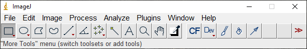
ImageJ is a free, open-source application developed at the National Institute of Health by Wayne Rasband to adjust and analyze high-resolution images of small structures. There’s a variation called “Fiji” (Fiji Is Just ImageJ) which bundles ImageJ with tools specifically intended for biologists. Happily, they are equally valuable for analyzing WSP. The interface can be intimidating, but only because there are so many functions that we won’t be using. The learning curve is worthwhile because the user has complete control over the analysis.
Three steps to image analysis
No matter the software, the operations used to analyze a digital image tend follow a three-step progression:
- Pre-processing: We select an ROI (a Region Of Interest) in the image and perform a few preliminary operations to improve image quality and contrast. In selecting a specific region, we can avoid unwanted flaws like drips or fingerprints as well as crop the image to some standard size for scaling purposes.
- Processing / Detection: Point and Morphological Operations are used to refine the image and establish a threshold so we can differentiate between deposits and the unstained background. The ideal outcome sees the original colour image converted to a binary (typically black and white) image.
- Measurement: We use ready-made computational routines to quantify some value. Typically, the percent area covered by deposits, but possibly the count and density of those deposits and perhaps even an estimate of the original droplet size.
Let’s explore each of these steps.
1. Pre-processing step
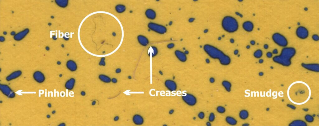
Pre-processing establishes the scale of the image and allows us to isolate the specific region we want to analyze. Perhaps the water sensitive paper was folded during sampling and we want to analyze each half separately. Perhaps we want to avoid obvious imperfections that would interfere with our results. In some cases, pre-processing might also include adjusting the image brightness to improve the contrast between stains and the yellow background.
2. Processing / Detection step
Processing and detection can take time because of the degree of computation involved. The higher the resolution and the larger the ROI, the longer it will take. Depending on what you want to measure, it might be acceptable to sacrifice some accuracy for speed.
We begin by determining which pixels represent part of a deposit stain and which represent part of the unstained background. We can accomplish this through global point operations called Thresholding and Filtering. If you haven’t already noticed, image analysis includes has a lot of jargon: “global” means the entire image and “point” refers to our focus on individual pixels. Ultimately each pixel is assigned one of two values, reducing the image to a binary (or 1-bit) format.
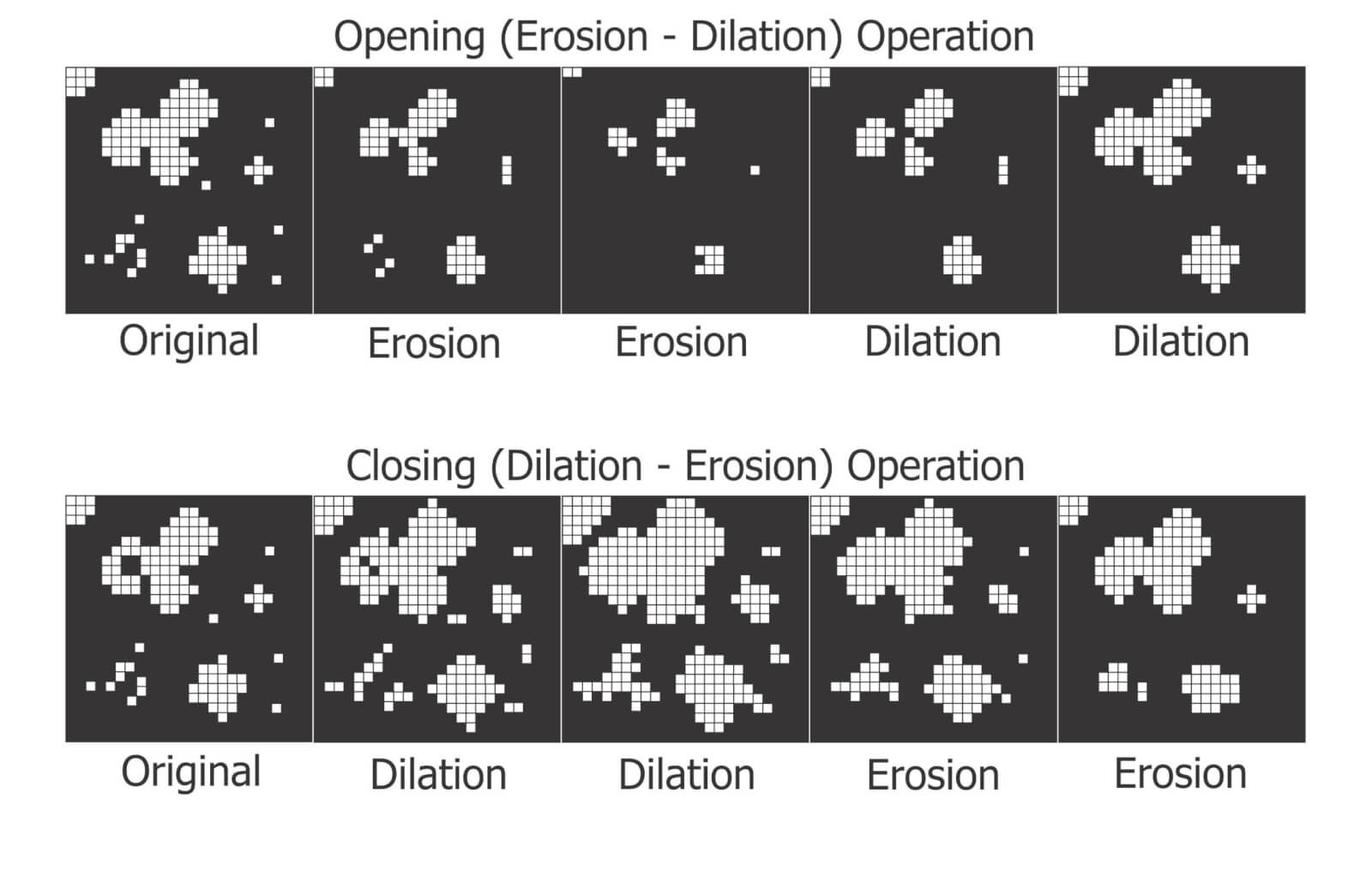
Once we have a binary image, we explore the shapes of the deposits (which are sometimes referred to as objects) to determine the limitations of what we’re confidently able to measure. Morphological operations are used to refine or modify these shapes in order to smooth jagged edges and identify whether an object is the result of a single deposition or multiple overlapping deposits.
3. Measurement step
Depending on the image analysis software, the user may be limited in what they can measure. The spectrum ranges from a single value (usually percent area covered) to in depth data relating to each object in the image. The latter might appear in a pre-formatted report, or as a CSV (Comma Separated Value) file for further exploration in spreadsheet format.
Thresholding
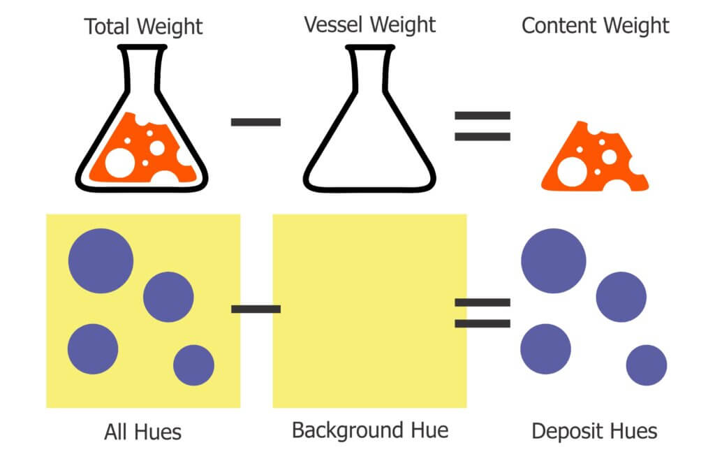
A thresholding operation sorts all the pixels in an image by some characteristic, and then allows us to set a threshold dividing them into two camps. In our case, we want to divide them into “stained” and “unstained”. The process is almost like taring a scale, where anything above the weight of the container is identified as the weight of the contents.
The HIS thresholding operation
ImageJ’s Colour Threshold operation is only one way to threshold an image, but it serves as a good example. This method uses HIS (Hue, Intensity and Saturation) to separate the deposit stain colours (blue-green) from the background colour (Yellow). As discussed, each pixel is represented by one or more 8-bit values. In this case pixels represent 0 – 255 hues, 0 – 255 intensities and 0 – 255 saturations. That may seem intimidating, but we mostly focus on hue.
When the Colour Threshold operation is selected, ImageJ sorts all the pixel values in the image into a binned histogram (where the Y-axis is the pixel count and the X-Axis is the range of pixel values).
a. Hue
We begin by considering the hue, which is simply another word for colour. An image with no stains would produce a histogram with pixel colours producing a distinct peak in the yellow range. An image with stains would also display peaks in the blue-green range. The user then segments the background from the foreground by manually setting the threshold between these peaks.
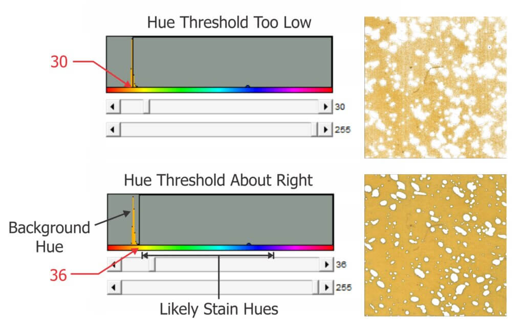
The hue thresholding process is less reliable (or can outright fail) when WSP has coverage in excess of 50%. This is because the color of the intermittent unstained areas changes as the distance between stains decreases. Think of it as blue bleeding into the yellow. The result is that the level of contrast between stained and unstained regions is inconsistent, making it difficult to confidently differentiate between “stained pixels” and “unstained pixels”. Similar issues arise when humidity causes the background colour to change but this tends to be more uniform and easier to threshold.
If the hue threshold it is set too low, stains will appear smaller and lose their shapes. If it is set too high, stains will appear larger and the gaps between adjacent, separate stains can disappear. This can have a significant impact on deposit count and distribution assessments, resulting in the loss of thousands of tiny, distinct deposits. Threshold accuracy has less impact on the determination of percent area covered. Research has shown that the use of a single threshold for multiple papers gives an absolute error of +/- 3.5% area covered. This is considered well within the intrinsic variability of spray coverage data.
b. Intensity
Sometimes referred to as “Value”, intensity can be thought of as pixel brightness. No threshold is required here because capturing the entire 256 pixel value range improves the contrast between colours.
c. Saturation
Finally, saturation (a measure of the difference between red, green, and blue levels) is a useful thresholding adjustment when WSP has been exposed to humidity. Humidity does not affect WSP’s ability to resolve stains, but as we mentioned it can cause the background to take on an overall greenish hue. An increase in low end saturation limit can increase the contrast between the stain colour and a less-distinct background colour.
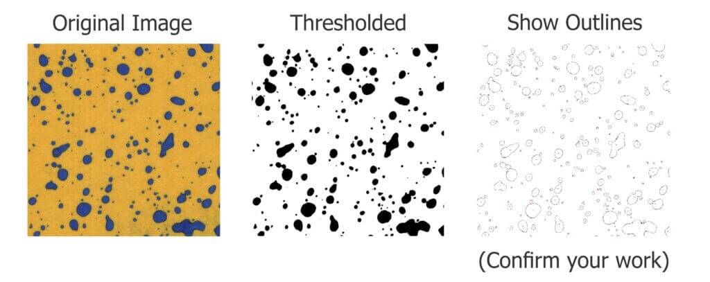
When the HIS thresholds are set, ImageJ converts the pixels values closer to the foreground (stains) to black and those closer to background (yellow) to white. Users can invert this if they wish, or even make the stains red. The important part is that we now have a binary image that makes a clear distinction between the stains and the unstained background. Ideally, thresholding should be performed for each consistent set of samples.
Learn how HIS thresholding is being used to perform weed recognition functions on sprayers in this article.
Pixel filtering
We won’t belabor filtering because it isn’t often required when analyzing WSP. Filtering operations compare pixel values to those of their neighbours and then replace those values with some form of weighted average. This reduces the relative differences between pixel values, smoothing the image and reducing noise (at the cost of lost detail).
Last article –Part three: Morphological Operations and Interpretation.