Category: General Concepts

For basics category

Operator Safety: How to Avoid Pesticide Hazards
A Veteran Applicator’s Questions about Pesticide Handling
Time and again, after years of working with dozens of different chemicals, I would wonder to myself “How dangerous is this chemical?”, “Is glyphosate as safe as they say it is?”, “How do I find out what type of safety gear I need while handling this chemical?”
Beyond the agrichemical dealer, ag. consultants, and university or government ag. extension specialists, a quick internet search reveals many sources of pesticide information. Collectively they identify the active ingredient(s) in formulated products, they detail which pests are best controlled by the pesticide, and they provide instruction for application. But it’s more difficult to find consistent, practical information about safe pesticide handling. Sometimes it’s excessive to the point of being impractical (try finding actual “chemical proof” gloves), and sometimes it’s minimal and vague – it depends where you look. No matter the level of precaution, pesticide safety is time consuming and involves some fussing, but it is the hallmark of responsible pesticide use. Just as we ensure that we are applying “safe rates” when spraying chemicals, we must also ensure we are respecting our own well-being while handling chemicals.
In Canada, the Pesticide Regulatory Directorate (PRD) is charged with protecting human health and safety by monitoring pesticides that are sold in this country. According to the Federal Pest Control Products Act all pesticides sold in Canada must be registered with the PRD. There’s a very nice overview of how that process works here. It is during this registration process that pesticide handling precautions are identified for the label. Further classification may take place under provincial acts.
All pesticides are designed to disrupt, repel, control or kill living organisms, but when it comes to safe handling, insecticides receive the most attention. This is because herbicides and fungicides target biochemical pathways that only exist in plants or fungi. However, most pesticides can be hazardous if they are not handled correctly. The handling precautions that appear on the label are based on five factors.
Five factors that affect handling precautions:
1. Pesticide Family
This factor is the broadest way to categorize potential risk to the handler. Generally, herbicides and fungicides are considered safer than insecticides, but there are notable exceptions. Do not rely solely on the pesticide family when making decisions on pesticide handling.
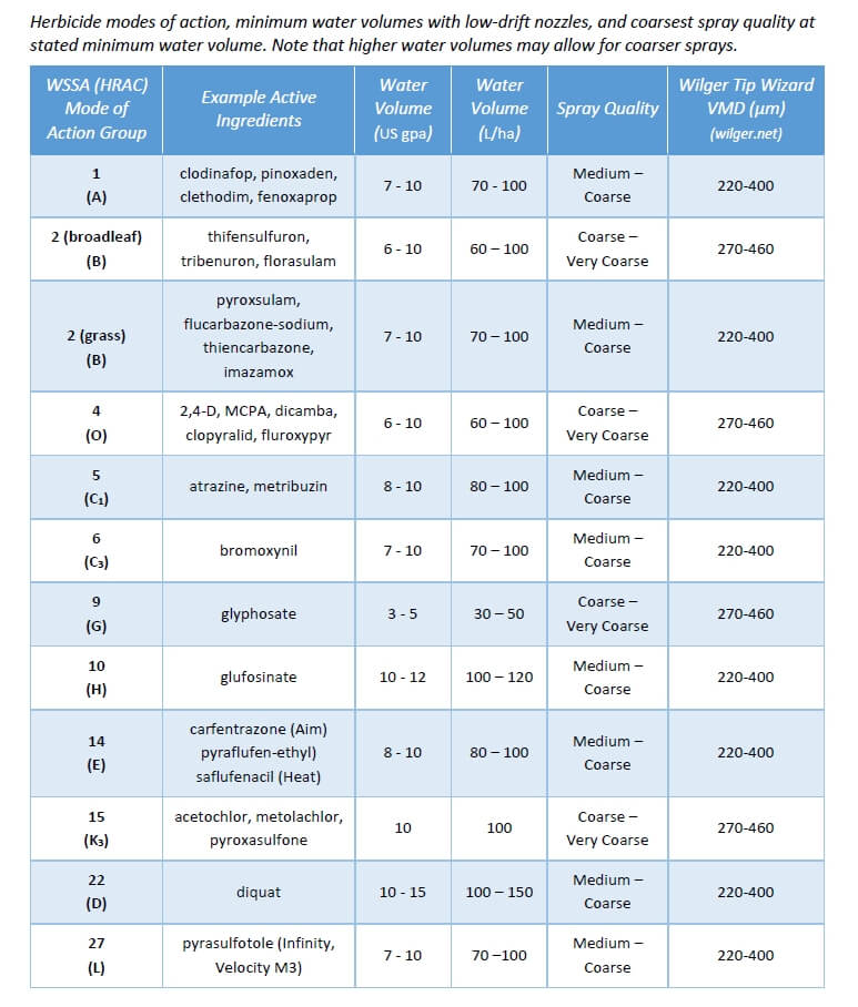
2. Pesticide Mode of Action
The mode of action gives further detail into how a pesticide should be handled. Modes of action that inhibit biochemical pathways that exist in the target pest, but not in mammals (people, in particular), have lower acute toxicities. Examples include herbicides that inhibit enzymes involved in amino acid synthesis or in photosynthesis – these enzymes do not exist in mammals. However, once again, there are always exceptions. Do not rely solely on mode of action when making decisions on pesticide handling.
3. Pesticide Formulation & Route of Entry
Pesticide formulation affects how a product can potentially be absorbed into the body. Emulsifiable Concentrates (ECs), for example, have higher rates of absorption than solutions or dry products. When it comes to the route of entry, dermal contact is considered safer than inhalation or ingestion. However, not all parts of your skin are created equal, and the point of dermal contact on the body matters a great deal.
4. Pesticide Toxicity
Taken collectively, the first three factors form the overall toxicity of the pesticide. The level of toxicity cannot be predicted – it has to be tested. The LD₅₀ (defined below) values that are reported for a pesticide come from standardized experiments such as animal feeding. Although the chosen species (usually white rats for mammalian endpoints) are known to be similar to humans in their response, there is still the possibility of error. Nevertheless, toxicity forms an important basis for establishing handling precautions.
5. Operator Exposure
People handle toxic substances every day. Household bleach, for example is surprisingly toxic, and yet it can be readily found on kitchen shelves in many homes. The risk of being harmed by a toxic product can only be determined by the likelihood of exposure. While it is possible someone might accidentally consume a hazardous dose of bleach, it’s improbable. Exposure does not just refer to a single exposure to a substance – repeated exposures to small doses of a toxic substance can have a cumulative effect. The goal when handling any pesticide is to minimize exposure, but it becomes even more critical when that pesticide is highly toxic. Together, exposure and toxicity form the basis for risk.
Risk = Hazard x Exposure
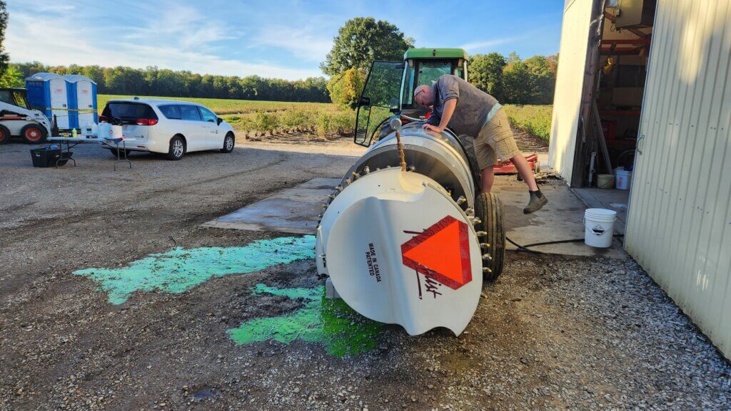
Studies have shown that exposure is greatest for handlers of agricultural pesticides during the mixing and loading phase of spraying. During this phase, the risk to the handler may be increased due to:
- physical stress
- the denial of risk
- a negative opinion of personal protective equipment (PPE)
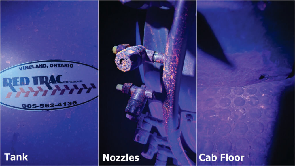
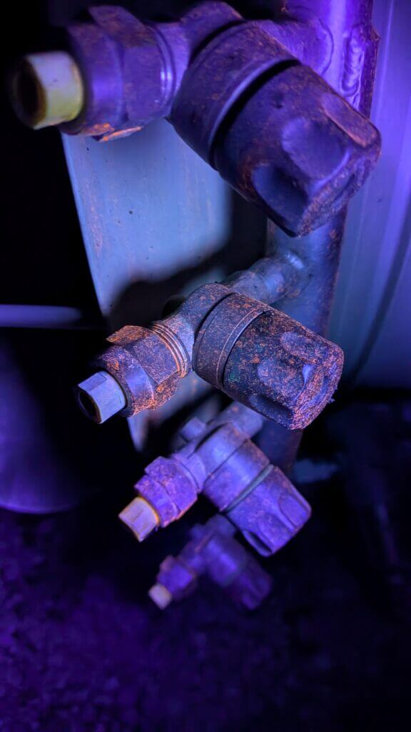
The main method of pesticide exposure is dermal, and many of the surfaces on a piece of equipment are already contaminated.
Health effects of pesticides: Acute and Chronic
Acute: short term
High exposure, resulting in immediate reaction due to a high dosage of pesticide exposure. The severity depends on the toxicity of the molecule and entry into the body (dermal, oral, eyes, etc.). The most common acute reaction is skin irritation, although in certain cases respiratory, digestive, and neurological systems may be affected. Organophosphate (e.g. Lorsban, Malathion) and carbamate (e.g. Sevin, Lannate) insecticides inhibit the cholinesterase enzyme, which is found in humans and affects nerve function. Frequent users of these insecticides undergo regular blood tests to ensure their levels are normal.
Chronic: long term
Chronic affects are more prolonged as they are usually due to lower doses of pesticide exposure over a longer period of time. Although some rare cancers and disruption of the reproductive system have shown to be related to this type of exposure, when the general population and farming population have been compared in studies, the farming population has shown an under-representation in the majority of cancers. In the cases were reproductive malfunctions were observed, a different cause of the malfunction, such as genetic offset, was most often observed in these situations. However, cancer types such as skin cancer and brain cancer were overrepresented in the farming community. A study in France has shown that the onset of neurological disorders in Agriculture communities shows a strong connection between Parkinson’s disease and exposure to pesticides.
Label Information
The majority of information needed to safely handle pesticides is found on the label. Pesticide labels are legal documents, meaning they can be enforced by the federal government. The problem is that most sprayer operators rarely look at the label as they are not very reader friendly and easy to skim through. Most pesticide boxes even have the recommended rate, or acres/case on the side of the box now, so there is even less reason to look at the label.
LD₅₀– the dose of pesticide in mg per kg of the test animals body weight that is lethal to 50 percent of the group of test animals. For example, if the pesticide has an acute oral LD₅₀ value of 1000 mg/kg, and the test animals each weigh 1 kg, then 50 percent of the animals would die if they each ate 1000 mg of pesticide at once. A 100 kg animal would need to ingest 100,000 mg (100 g) of the pesticide for the same effect. LD₅₀ is often expressed by the route of entry – dermal, inhalation, acute oral (ingestion) are the main examples.
Degree of Risk and Hazard Symbols
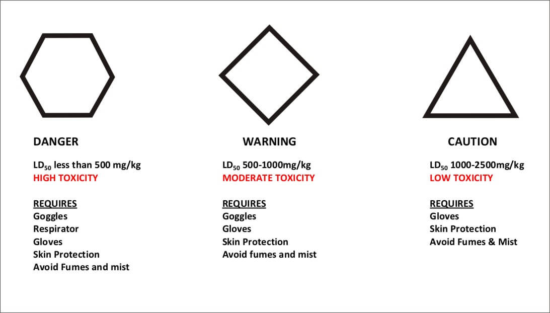
Two Factors that Determine the Appropriate Level of PPE
1. The Hazard Rating (above) incorporates the minimum protection generally required for a substance with the rating.
2. The Label Recommendations will usually give the additional specific protective clothing and equipment needs for an applicator.
Degree of Exposure
This increases as the length of each pesticide application increases. As the number of pesticide applications increases, the time between exposures decreases. If an operator becomes exposed to spray, dust or fumes the degree of exposure increases. Essentially, more protective wear is needed as the degree of exposure becomes greater.
Knowledge
This encompasses all of the above information. In order for a pesticide applicator to avoid injury or the chances of adverse effects on the body, a pesticide applicator must be knowledgeable about pesticides. It can be overwhelming for an applicator to sort through all of the information on the label or on-line regarding pesticides. So much so, that most often applicators avoid the information altogether. Ongoing training and learning will ensure that they are effective in their work. Many aspects of pest control change continuously, as new studies are conducted on the effects of pesticide exposure.
A Safety Data Sheet (SDS) is available for each pesticides registered, and these are usually linked on manufacturers’ websites. It can be eye-opening what types of toxicity tests are done, and what the results are.
Denial that pesticides can potentially cause harm is also a major flaw in the behaviour of applicators. Maintaining a safe work environment and practicing personal safety will reduce the chances of an applicator experiencing serious injury throughout their farming career.
Unknowns
There is very little certainty in toxicology. For one, most testing is done using acute oral and dermal dosing. Basically, toxicologists expose test animals to the neat active ingredient and watch what happens. There is a lot of missing information – what about formulant like solvents, and surfactants? What about synergies in tank mixes? Some, but not all of these, undergo testing. We also have much less information on chronic (long-term) effects, and can only simulate these in quasi long-range tests. In addition, toxicological methodologies and statistical approaches can vary, and we should not be surprised that some reports disagree, and that there are outright conflicts between toxicologists and epidemiologists (scientists that study patterns of health in populations). Regulators are aware of these shortcomings and often use safety factors to account for them. But those of us that use these products regularly, the message is simple: be cautious, and protect yourself.
Avoid Cross-Contamination
Disposable nitrile gloves are the product of choice for handling pesticides. But one of the most common problems with the use of gloves is cross-contamination. You’re handling product with your gloves on, touching containers, hoses, valves, and couplers. When you’re done, you climb back into the cab where you take off your gloves. Later, someone climbs up into the cab to talk to you, using the railing and operating the door handle without gloves. Guess what’s on their hands? Even later, you put away the hose without gloves and return to the sprayer. Now it’s on the steering wheel and all the levers. There are a few solutions:
- Double-glove so you can take the dirty outside glove off and still be protected.
- Wipe down surfaces that you might touch with gloved or bare hands daily.
- If using non-disposable gloves, avoid lined gloves and rinse the insides out daily.
Learn More
If you would like to learn more about pesticide safety, or to obtain pesticide application training, the Pesticide Applicator License can be obtained from the Ministry of Agriculture. This course offers in depth, valuable safety information for applicators, as well as general knowledge for pesticide applicators. The Pesticide Regulatory Directorate provides workers, employers, and the general public with a wide range of pesticide information. The PRD can be contacted from anywhere in Canada toll free at: 1-800-267-6315
Download this Quick Reference Guide for commonly used herbicides. Print, laminate and post it at the fill station or pesticide storage area for easy reference. Also, grab a copy of Health Canada’s “Stay Safe when using Pesticides” factsheet.
Sources
May 11, 2026

Comparing Fluorescent Dyes for Spray Coverage Evaluation

I work in agricultural extension and I’m always on the lookout for new methods to help me achieve my goals. A big part of my job is to research and teach efficient, effective and safe crop protection practices, so it follows that I have to be able to evaluate the quality of a spray application. Fundamentally, there are two ways to do it:

Wait to see if the pesticide did its job and protected the crop from weeds / bugs / disease.
Don’t wait. Confirm your spray is depositing where you want it before committing to the application.

Three guesses which approach I advocate. So, how do you check spray coverage in a way that’s quick, cheap, easy and informative? Again, there are choices, but rather than simply list them I’ll add a little insight in the form of pros and cons.

Method	Pros	Cons
Water sensitive paper	Relatively cheap, available, clean, easy, repeatable, supports a photographic record, simple to analyze.	Does not accurately reflect coverage on plant surface, slow to place and retrieve, can be spoiled by dew, humidity and physical contact.
Inspecting for residue / wetness	Cheap and fast.	Not proactive, too subjective, not repeatable, pesticide many not leave visible residue, requires re-entry soon after spraying.
Inspecting spray pattern (e.g. shoulder check)	Cheap and fast.	Not proactive, not indicative of coverage, not repeatable.
Watching for run-off	Just don’t.	Just don’t.
Fluorescent dyes	Reflects actual, whole-canopy coverage and off-target coverage at same time.	Expensive, hard to find, messy, time-consuming, hard to photograph, not repeatable, leaves unwanted residues (or can’t be used on edibles), may have to take place at night, may fade quickly… *or is any of this actually true?*

I’ve never been a proponent of spraying dyes because of the reasons I listed in the table. If I already have difficulty convincing a grower to leave the sprayer or tractor cab to place and retrieve water sensitive papers, what are the odds of them mixing a messy and expensive tank of dye and waiting until twilight to see the results?

On the other hand, dyes are compelling. Particularly if we change the perspective a little. What if we consider the use of dyes, not as a tool for a grower, but as a tool for agricultural extension or consultation (really, anyone that wants to research or teach the safe and effective use of crop inputs)? Several of the cons are minimized or even eliminated. Additionally, this new lens reveals several uses for dyes beyond spray coverage. This is not an exhaustive list:

Off-target (primarily drift) evaluation
Dermal exposure / PPE evaluation
Rinsate / sprayer cleanout evaluation
Sprayer loading / point source contamination evaluation

I decided to compare a few of these dyes. I enlisted the help of a local blueberry operation. Being October, all the berries have been picked so we could spray the bushes without any risk to the fruit. Plus the sprayer was clean and the growers were curious to evaluate their spray coverage.

Having secured a location, spray equipment, and operator, I needed dyes and some criteria for choosing them. First and foremost, I chose fluorescent dyes that glowed under UV (aka black lights). My thinking was that they would be more interesting in demos, and given that we might be spraying horticultural operations, I didn’t want obvious and persistent stains on the produce. At least not something easily seen in daylight before it broke down and/or was washed away.

My UV dye candidates had to be:

Moderately inexpensive.
Non-toxic (i.e. had an SDS that clearly permitted human exposure, were environmentally friendly and could be sprayed on edible crops).
Readily available in Ontario (e.g. quickly and cheaply shipped from within Canada or perhaps the US).
Available in formats that facilitated small volume batches (anywhere from 50 mL squirt bottles for indoor demos, up to 50 L volumes for field demos).
Clearly visible on plant tissue.

I found five likely prospects for the study. I won’t list prices, but none of them were over $100.00 CAD. Number 3 was a free sample and number 5 was gifted to me by a colleague more than 15 years ago. I looked up the SDS for that last one and was surprised that it was relatively inert. So, I used it.

Dye number	Name of dye	Commercial size	Manufacturer	Location
1	IFWB-C81PT	1 pint	Risk Reactor	California, USA
2	UVTRACER-G1PT	1 pint	Risk Reactor	California, USA
3	Eco Pigment Blaze Orange SPL15JX	Sample size – 100 grams	DayGlo	Cleveland, Ohio, USA
4	Fluorescent Yellow Tempura Paint	1 liter	Tri-Art Manufacturing	Kingston, Ontario, CA
5	Phosphor Powder (Zinc Orthosilicate: Manganese CAS#11-47-2)	1 kg	Global Tungsten and Powders Corp.	Pennsylvania, USA

I also purchased UV lights. When I was bequeathed the phosphor powder it came with heavy, ancient, black lights. They made an unsettling humming noise and required a power source, making them unwieldly for field work. I opted to try three battery powered versions instead. Again, I won’t list prices, but they weren’t unreasonable.

UV flashlight number	Name of light	Manufacturer	Wavelength / wattage	Batteries
1	Super Tac	Risk Reactor	395 NM / 850 µW/cm² at 5 inches	Rechargeable battery provided
2	Mini Zoom	Risk Reactor	395 NM / 1 watt	1 AAA
3	V3 UV Flashlight with 68 LEDs	Amazon.ca	395 NM / 10 watts	3 AA

Regarding the recipes, one of my criteria was that the dyes could be mixed in relatively small batches. I chose 50 L as the high end because the airblast sprayer we were using (Turbo-Mist 30P) could still prime when only 50 L was added to the tank. This allowed us to mix as small a batch as possible, while still having enough to spray a row of berries from both sides. We left three rows between treatments to serve as buffers.

Turbo-Mist Model 30P before the dye-job.

I also had to consider the nature of the dyes. The Eco Pigment (Dye 3) is a hydrophobic powder and two colleagues warned me that it was notorious for plugging filters. So, it had to be mixed with a non-ionic surfactant (NIS) to help “wet” the powder prior to adding it to the tank. In fact, NIS seemed like a good idea for all my dye candidates, so I included Activate Plus (Sollio Agriculture, Winfield Solutions) in each recipe.

I added the dye, NIS, and a small amount of water to a Pyrex measuring cup on a digital scale, then rinsed the cup into a final volume of 50 L while filling the tank. I didn’t always follow the advice I received, so I’ll show you the ratios I was told and (right or wrong) what I ultimately did.

Dye number	Manufacturer- or colleague-suggested ratio	Amount of dye	Amount of NIS	Amount of water
1	1 part dye : 10,000 parts water	125 mL	65 mL	310 mL
2	1 part dye : 10,000 parts water	125 mL	65 mL	310 mL
3	1 gram dye : 1 mL NIS : 200 L water	65 grams	65 mL	425 mL
4	1 part paint : 100 parts water	500 mL	65 mL	0 mL
5	1 gram dye : 1.25 L water	65 grams	65 mL	425 mL

It took roughly 15 minutes to fill, prime, spray, and rinse out each dye. We started at 5:00 p.m., were done at 6:15, and then waited for sunset at 7:30.

50 L tank mixes going through circulation and paddle agitation.

Draining the remains and rinsing the tank. It looks terrible, but these dyes are intended for environmental projects like tracing water courses.

We used a smartphone (Google Pixel 9a – 48 megapixel camera) to photograph each combination of dye and flashlight. It was tricky to find an angle where the black light illuminated the residue, but didn’t wash out the photo. In those cases where the dye was evident, it was always far more vibrant in person than through the lens of a camera. As for the results?

Lets start with the lights. We found that the high wattage of Light 3 showed dye more easily. This also happened to be the cheapest light, which was a pleasant surprise.

Dye 1 and 2 were disappointing. We couldn’t see anything on the plants. This dye is intended for monitoring plumbing and water courses, and the manufacturer states that the colour will disappear if the solution is mixed with chlorine. Perhaps mixing it with city water caused it to fade, but that’s likely to happen, so these dyes failed.

Dye 1 – Light 1, 2 and 3. A sad, single drop showed up for Light 3.

Dye 2 – Light 1, 2 and 3. Again, a solitary deposit illuminated under Light 3.

Dye 3 was spectacular. Not only was it evident with every light source (including day light to some extent), but we were able to find it several rows downwind, on the sprayer nozzles, all over the tires and on the floor of the cab (which surprised the operator). I may have mixed this one too strong; It seemed to clump on the leaves, but perhaps that’s because they were exceptionally waxy.

Dye 3 showed up everywhere… whether we wanted it there or not.

Dye 4 came in second place. It wasn’t amazing, but it was visible. This is children’s tempera paint, used in daycares for finger painting and at universities for raves. I’ve used it in the past with mixed results, not only to spray canopies, but in classroom demos on cabbage leaves and as a surrogate tracer to hunt down where pesticide hides in sprayer plumbing. It’s OK in a pinch if you mix it at least 2x more concentrated than I did here.

Dye 5, like dyes 1 and 2, was a disappointment. I’ve seen it used in powder-form to demonstrate how dermal exposure can spread as you touch clothing, doorknobs, your face, and places where the occasional adjustment is required. But in a liquid solution, it wasn’t any good at all.

Persistence

We followed up after the application to see if the dyes would persist. Twenty four hours after application, Dye 4 (our runner-up) was gone. This was no surprise given it was a water soluble paint and wasn’t terribly showy to begin with. However, Dye 3 (our winner) was still clearly in evidence. This is a hydrophobic, micro ground powder (~0.1 micron). That’s one reason it had to be mixed with a non-ionic surfactant. The following photos shows little or no change after 24 hours and a respectable dew:

Three days after application (DAA), we had a rain event. Four DAA this (blurry, sorry) image was taken:

We see that the deposits did redistribute to drip points and the overall coverage was reduced, but it was still holding on. This means it likely shouldn’t be used on any horticultural crop that isn’t going to be washed. Or at least used long before any fruit, leafy green or vegetable contacted by the powder will be harvested. Not because it is unsafe (see safety data sheet) but because of the optics to buyers.

Conclusion

And so, I hope you have been inspired by this process. I’ve learned that the use of dyes for education and research is potentially powerful, relatively cheap, and more accessible than I originally thought. Certainly the growers were impressed by what they could suddenly see and it’s led them to reassess some of their practices. Just bear in mind the possible persistence, and remember to wear gloves when mixing.

Thanks to Mark Ledebuhr, Helmut Spieser, David Manktelow, and Ben Werling for the helpful advice. Thanks to Brandon and Jordan Falcon for use of their spray equipment and their blueberry operation.

October 2, 2025

Fungicides and Integrated Pest Management – An Apple Scab Case Study
Editor’s note: This article originally appeared in the Winter, 2025 ONCore newsletter (Volume 29, Issue 1). We thought it was an excellent description of the integrated pest management process and where fungicide spraying fits in. It’s been modified from the original version.
Part One: Know Your Enemy
There is no denying that product efficacy and rotational partners are critical components of effective pest management. A pest is causing damage; we need as many tools as possible to control it. Let’s consider the basics of Integrated Pest Management (IPM). The first step in effective management is understanding the pest biology.
Figure 1. Foundations of integrated pest management
Let’s use apple scab as a case study for the IPM process. We’ll start with a deep dive into apple scab 101 by referring to its typical life cycle. Apple scab overwinters in infected leaves on the orchard floor. During the winter and early spring, immature ascospores (primary inoculum) are protected in specialized spore sacs, called pseudothecia.
Figure 2. Life cycle of apple scab (Image: Cornell University)
Maturation of ascospores in the leaf litter on the orchard floor usually occurs at the same time the trees are emerging from dormancy. This means mature ascospores are present and ready to infect the first green tissue in spring. However, the percentage of mature ascospores in the orchard generally peaks when apples are at the late pink to petal fall stages of bud development.
Once the tree breaks dormancy and green tissue is present, a primary infection occurs if the following three conditions are met:
1. Mature ascospores are present in leaf litter in the orchard.
2. Weather conditions favour ascospore discharge and infection.
3. Fungicide protection is inadequate to prevent infections.
Mature ascospores are discharged from the pseudothecia by rain and splashed up to emerging green tissue by wind. Moisture – dew or rain – is necessary for ascospore discharge and germination, as well as subsequent infection of apple tissue. Olive green, velvety lesions appear 10-28 days after infection by an ascospore, depending on temperature. The lesions initiated by ascospores result in primary infections, and in turn, produce spores called conidia.
Conidia are spread from primary lesions by rain or wind and initiate further infections when the combination of temperature and leaf wetness enables them to germinate and become established. These are called secondary infections, and generally occur within a tree or between adjacent trees rather than at a long distance.
The secondary cycle can be repeated many times during the growing season, whereas primary infection only continues until all overwintering spores are depleted. With frequent rainfall, the control of apple scab becomes extremely difficult as the season progresses, particularly if the disease becomes established from primary infections in the spring.
Early season management (green tip to tight cluster) provides the greatest economic protection against loss from scab control failure. In other words, don’t wait to get fungicide protection on!
Figure 3. Risk of primary apple scab infection and the probability of economic loss from scab control failure. (Image: Cornell University)
Part Two: When To Strike
Just like how understanding the biology of the pest helps to determine appropriate intervention timings, understanding how fungicides work will help determine when best to apply them and ensure maximum efficacy (aka the most bang for your buck).
Fungicides can be divided into four categories, based on what they do:
1. Preventative
2. Curative
3. Eradicant
4. Antisporulant
Preventative
- Before the plant is even infected
- Before we can see any symptoms
- Most fungicides work preventatively
- If fungicides work in multiple ways, often they work best preventatively
Curative
- Stops the mycelial growth inside the plant
- Still can’t see any symptoms
- Fungicides with “kickback”
Eradicant
- Stops the pathogen during lesion formation
- Ok, now we can see symptoms
- Very few fungicides work this way, even though this is how we expect them to work
Antisporulant
- Stops the pathogen from sporulating
- We can see symptoms
- Several fungicides work this way, but your crop is already infected
In addition to the timing of a fungicide, efficacy can be affected by residues (or lack of), rains and risky gaps. A general rule of thumb often used is that 1 inch (2.5 cm) of rain removes approximately 50% of protectant fungicide residue and over 2 inches (5 cm) of rain will remove most of the residue. While systemic fungicides tend to perform better than protectant (or contact) fungicides in rainy periods, they do still require a certain amount of time prior to a rain event to be taken into the leaves – which isn’t always as easy as it sounds (see Part three).
During conditions conducive to disease development, it is important to maintain tight intervals between fungicide applications. Most labels will have the minimum interval listed. For protectant fungicides, a tight interval program would be 5-7 days. Where possible, do not extend intervals beyond 14-21 days if there are any concerns of disease. As a fungicide application ages, the efficacy of that product is reduced.
Spray coverage can be affected by wind in several ways:
- Wind direction – can carry droplets away from intended target
- Wind speed – affects how far the droplets travel
- Consistency – wind gusts can make coverage inconsistent
In addition to wind, spray coverage can also be affected by water volume, nozzle orientation, sprayer calibration, alternate row spraying, etc .
Areas of the canopy that are often missed due to poor coverage are within the tree due to spray not reaching through or at the top of larger trees . Routine monitoring can miss early signs of scab infection in these parts of the tree if not done thoroughly. I saw numerous situations this year (2025) where scab lesions were overlooked.
Part Three: Fungicide Playbook
Let’s take a closer look at some common scab fungicides and what is meant by contact and systemic activity and how they might redistribute after application. The rest of this article refers to pesticide brands available in Canada. They may have different names in other countries.
Figure 4. Movement of fungicide in plant: (A) contact or protectant; (B) xylem-mobile or acropetal; (C) translaminar; (D) phloem-mobile. (Adapted from K. Goldenhar, BCMAF)
Contact (Protectant) Fungicides
These products remain on the surface of the plant tissue and provide preventative activity only. Examples of contact fungicides include fluazinam (Allegro, Vantana), coppers, sulphurs, mancozeb (Manzate, Penncozeb, Dithane), captan (Maestro, Supra Captan) and folpet (Folpan, Follow).
Unfortunately, because these products provide superficial coverage only, they can be prone to UV degradation or run-off and need frequent applications. Stickers/spreaders can help these stay on the plant but always refer to the label before using.
Systemic Fungicides
Systemic fungicides get taken up into the plant. Unlike contact fungicides, systemic fungicides tend to have longer duration and are rainfast once absorbed. However, sufficient tissue is needed for absorption so these products are best used after tight cluster in apples. How systemic fungicides move within the plant can vary:
Xylem-Mobile
Xylem-mobile, or acropetal fungicides move to the actively growing tips of expanding foliage and protect new growth. Examples of xylem-mobile fungicides include most Group 3 and 11s, as well as some Group 7s (e.g., fluopyram).
Translaminar
Translaminar fungicides move from the top of the leaf to the underside. Because of this limited movement, coverage matters. Examples of translaminar fungicides include most Group 7s as well as Cevya and Inspire Super.
Phloem-Mobile
Phloem-mobile, or “true” systemic fungicides move into the tissue and are carried to the roots to protect against root rots. There are no examples of phloem-mobile fungicides for apple scab. However, this group includes products such as Aliette and Phostrol which are registered for other diseases of apples. Unlike other systemic fungicides, this group has a short duration of activity (i.e., they move fast).
Resistance Management
Fungicides are grouped based on their mode of action, or how the product affects the disease. For example, all products in Group 3 have the same mode of action, so using one product is virtually the same as using all other products within that group. In pre-mix fungicides, both groups need to be considered in all rotation decisions.
Figure 5. Systemic fungicides registered for apple scab in FRAC Groups 3, 7, 9 and 11
One key strategy to good resistance management is rotating between products of different chemical groups. Figure 5 shows which fungicides belong to Groups 3, 7, 9 and 11. For instance, since Aprovia Top belongs to Group 3 and 7, it should not be followed by other Group 3 (Cevya, Fullback, Nova), Group 3+9 (Inspire Super), Group 7 (Excalia, Fontelis, Kenja, Sercadis), Group 7+9 (Luna Tranquility) or Group 7+11 (Merivon, Pristine).
For resistance management:
- Where possible, include at least half rate protectant fungicide.
- Do not use products containing the same chemical group in consecutive applications.
- Limit number of applications per group per season, where possible.
- Apply preventatively; do not rely on systemic fungicides for post-infection activity
- Do not use Group 3 (Nova, Fullback, Inspire Super) or Group 11 (Flint, Pristine, Merivon) fungicides after bloom for scab management as they are weak on fruit scab. Trials with Cevya have indicated good efficacy on fruit scab.
- Research from northeastern US indicates Group 7 fungicides may be weaker on fruit scab as well.
Part Four: Final Considerations
In conclusion, take some time to consider the following:
- Early intervention remains the cornerstone of effective disease management!
- Use weather monitoring tools to time fungicide applications
- Adjust spray schedules and product choice according to the weather
- Dedicate time for regular orchard inspections
- Train your team to identify symptoms early, accurately and consistently
- Optimize your spray program
- Protectant AND systemic fungicides
- Rotate classes to prevent resistance
- Select for broad-spectrum efficacy
- Reduce overwintering inoculum
The author gratefully acknowledges Katie Goldenhar, OMAFA Pathologist (Horticulture) for providing source material for this article.
May 22, 2025
Airblast Productivity and Work Rate Calculator
There are many factors that affect the work rate of an airblast application. If an operator can improve their work rate, without compromising spray efficacy or safety, they improve operational efficiency and save money.
But how does each variable factor in? Is it worth the cost of a tender truck and operator to fill more efficiently? Should you upgrade to a multi-row sprayer? Should your next planting have longer rows? We have a simple calculator that can help you make these decisions. You can build and compare multiple scenarios to explore the relative impact of small changes to your typical spray program. We recommend making only one change for each scenario so you can better understand the results. Print the comparison page for your records.
Whether you’re a sprayer operator, or a manager of sprayer operators, this exercise will help you see your spray program in a whole new light. Download a copy of the Airblast Budget and Work Rate Calculator and explore your productivity. You must have Excel to run the spreadsheet, and you must permit the use of macros (you’ll be prompted to accept).
Spoiler: It’s amazing how changes to travel speed have only a marginal impact on work rate. Often less than 60% of the total spray job is spent actually spraying!
If you’d like to see just how productive you can be, check out this rare (possibly unique) sprayer from Ed Oxley Farms in Michigan. Built on an OXBO 7550, this sprayer is the fourth iteration of a concept developed over the last 20 years by Ed Oxley Farms and ag engineers from Michigan State University.
Capable of spraying five rows at a time, this self-propelled beast is a hybrid wrap-around and targeting-tower system that uses CurTec spray heads equipped with tangential fans and wire-mesh basket rotary atomizers.
That’s not dribbling – that’s purging the boom prior to spraying.
It sprays a mere 150 L/ha (~ 15 gallons/acre) at a ripping 13 km/h (~8 mph), as seen on the Ag Leader monitor below.
When row spacing and turn time are accounted for, that means it’s capable of covering almost 15 hectares (~40 acres) per hour.
And, when not spraying grapes, the boom can be swapped to make it a high-clearance corn sprayer. It doesn’t get much more efficient than this.
The following videos will show the view from inside and outside the cab. Note that the row that’s straddled is sprayed from an overhead spray head mounted to the centre rack behind the sprayer. The two adjacent rows are covered from one side from vertical spray heads mounted on the chassis. Finally, the boom holds two more overhead spray heads for the outer-most rows.

Ideally, the boom-mounted spray heads would be suspended vertically inside the row, but it makes for such a wide turn radius that it would take too long to turn… assuming there was enough headland to allow it. They’re also swept-back to minimize the turn radius and reduce the amount of airborne spray that deposits on the sprayer itself.
A clever design that makes a few compromises to ideal coverage in order to improve productivity. The balance works for them and this sprayer might be a sign of things to come in horticultural crop production systems. Want to see how your sprayer stacks up? Download the calculator and see where you might be able to make improvements.
August 12, 2024
Mode of Action and Spray Quality
The decision on which application method is best for herbicides boils down to two main factors: (a) target type and (b) mode of action. In general, it’s easier for sprays to stick to broadleaf plants on account of their comparatively larger leaf size and better wettability compared to grassy plants. There are exceptions, of course – at the cotyledon stage, broadleaf plants can be very small and a finer spray with tighter droplet spacing may be needed. Water sensitive paper is a very useful tool to make that assessment. Imagine if a tiny cotyledon could fit between deposits – that could be a miss!
Some weeds are also more difficult to wet, and those may also need a finer spray or a better surfactant for proper leaf contact. An easy test is to apply plain water to the leaf with a spray bottle. If the water beads off or the droplets remain perched on top in discrete spheres, the surface is considered hard to wet. Most grassy weeds are hard to wet, while most broadleaf weeds are easy to wet.
Grassy weeds are an especially difficult target because they have smaller, more vertically oriented leaves, and almost without exception are more difficult to wet than broadleaf species. All these factors call for finer sprays for effective targeting and spray retention.
Broadleaf weeds usually have more horizontally oriented leaves which also happen to be larger. As a result, they can intercept larger droplets quite efficiently.
There are about thirty mode of action (MOA) groups among the herbicides with about ten accounting for the majority in Canadian prairie agriculture. It’s probably an over-simplification to categorize them into just two groups – systemic and contact. But that grouping goes a long way to making an application decision.
Contact products (MOA Group 5, 6, 10, 14, 22, 27) must form a deposit that provides good coverage. Good coverage is an ambiguous term that basically means that droplets need to be closely spaced and cover a significant proportion of the surface area because their physiological effects occur under the droplet, and don’t spread far from there. One way to generate more droplets is to reduce droplet diameter, another is to add more water. A reasonable combination of both is ideal because simply making droplets smaller creates issues with evaporation and drift.
Systemic products (MOA Group 1, 2, 4, 9) will translocate within the plant to their site of action after uptake. As a result, coverage is less important as long as sufficient dose is presented to the plant. In practice, this means coarser sprays and/or less water may be acceptable.
When two factors are combined, either in a tank mix or a weed spectrum, the more limiting factor rules. Application of a tank mix or product that is active on both broadleaf and grass plants will be governed by the limitation placed on grass targets. A tank mix comprised of both systemic and contact products is governed by the limitations placed on contact products.
A factor we should also consider is soil activity and the presence of residue. Studies have shown that soil-active products are relatively insensitive to droplet size. But if they have to travel through a layer of trash to get to the soil surface, more application volume is the best tool.
Below are some recommended spray qualities and water volumes for use in Canada. The spray qualities listed in the table can be matched to a specific nozzle by referring to nozzle manufacturer catalogues, websites, or apps. Note that Wilger also offers traditional VMD measurements on their site, allowing users to be a bit more specific if necessary.
Click here to download PDF
February 9, 2023