Tag: speed

  • How Higher Speeds Affect Drone Swath Width

    How Higher Speeds Affect Drone Swath Width

    Speed Study

    Swath width is a fundamental parameter in spray drone mission planning. It facilitates the uniform application of broadacre pesticides at the target rate. Pilots adjust the swath width via operational settings such as droplet size, flight speed and altitude to produce the most effective and efficient application.

    Rapid advances in drone design, however, may warrant a re-evaluation of how operational settings affect swath width. For example, the most recent generation of drones are now capable of speeds up to 20 m/s (72 km/h), which is twice that of the previous generation.

    In late 2025 we conducted a series of comparative herbicide applications using the DJI Agras T50 and T100. For both drones, swath width increased with speed up to ~10 m/s, as expected. However, between ~10 m/s and 18.5 m/s, swath width from the T100 did not seem to increase further. Similar observations have been reported by researchers at AgroEfetiva (São Paulo, Brazil; personal communication).

    These results suggest that the relationship between speed and swath width is positive and direct at lower speeds, but reaches a saturation point beyond which any further increase in speed no longer affects swath width. This is an asymptotic relationship. To test this hypothesis, we conducted a deposition study where swath width was measured at flight speeds that increased incrementally from 8 m/s to 20 m/s.

    Configuration Study

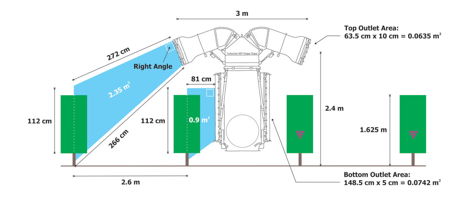
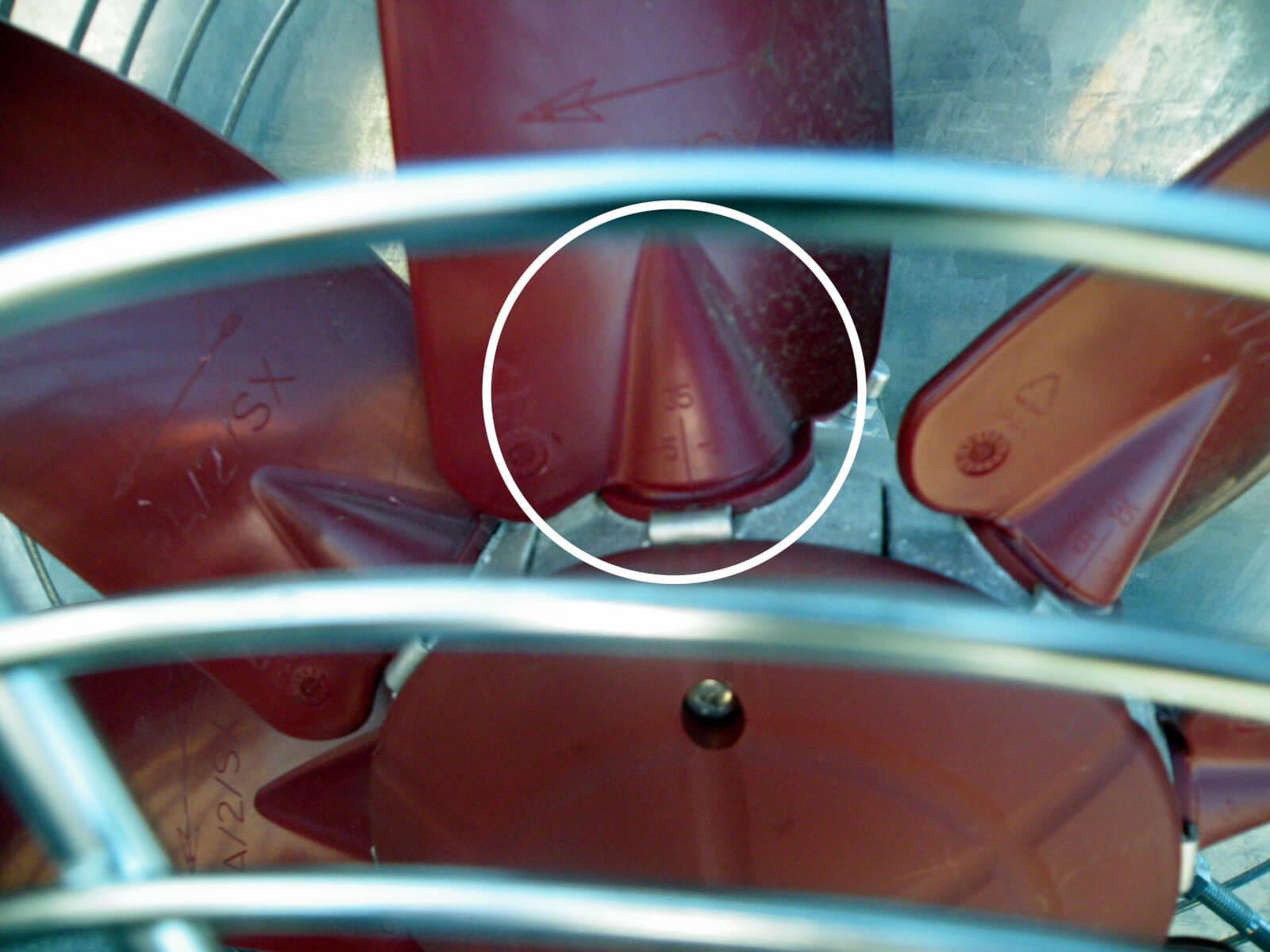
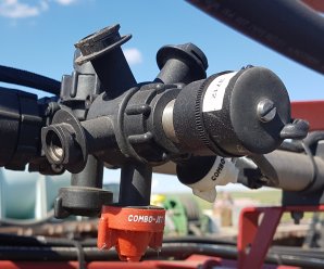
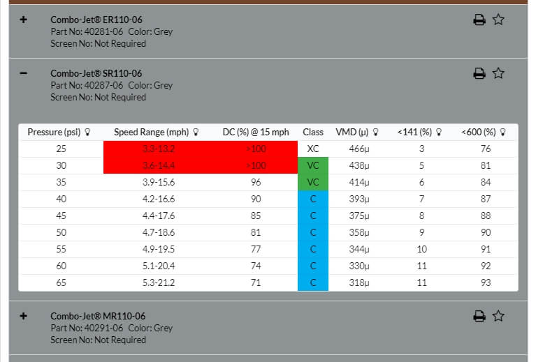
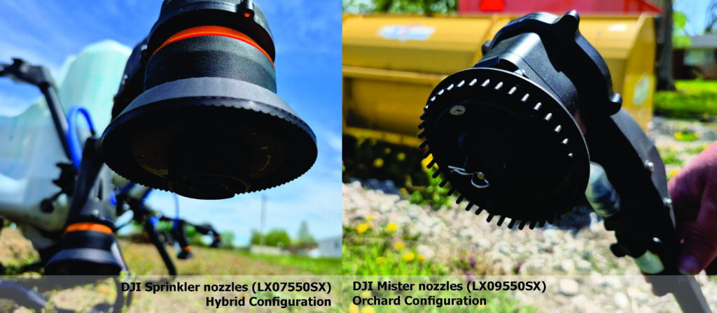
    The standard T100 configuration uses two rotary atomizers (“sprinkler” nozzles; LX07550SX) with a reported maximum combined flow rate of 30 L/min. The alternate orchard configuration incorporates a boom that supports two additional “mister” nozzles (LX09550SX), increasing the reported maximum flow rate to 40 L/min.

    To improve productivity in broadacre applications, some operators have adopted a hybrid configuration. In this setup, the orchard boom is retained, but the reputedly drift-prone mister nozzles are replaced with a second set of sprinklers. This approach is intended to achieve a higher flow rate than the standard two nozzle configuration while maintaining a larger mean droplet size.

    A secondary objective of this study was to compare the Hybrid configuration with the Orchard configuration (Figure 1).

    Figure 1 – Left: DJI Sprinkler Nozzle (LX07550SX). Four such nozzles comprised the “Hybrid” configuration. Right: DJI Mister nozzle (LX09550SX). Four such nozzles comprised the “Orchard” configuration.

    Materials and Methods

    Location and Layout

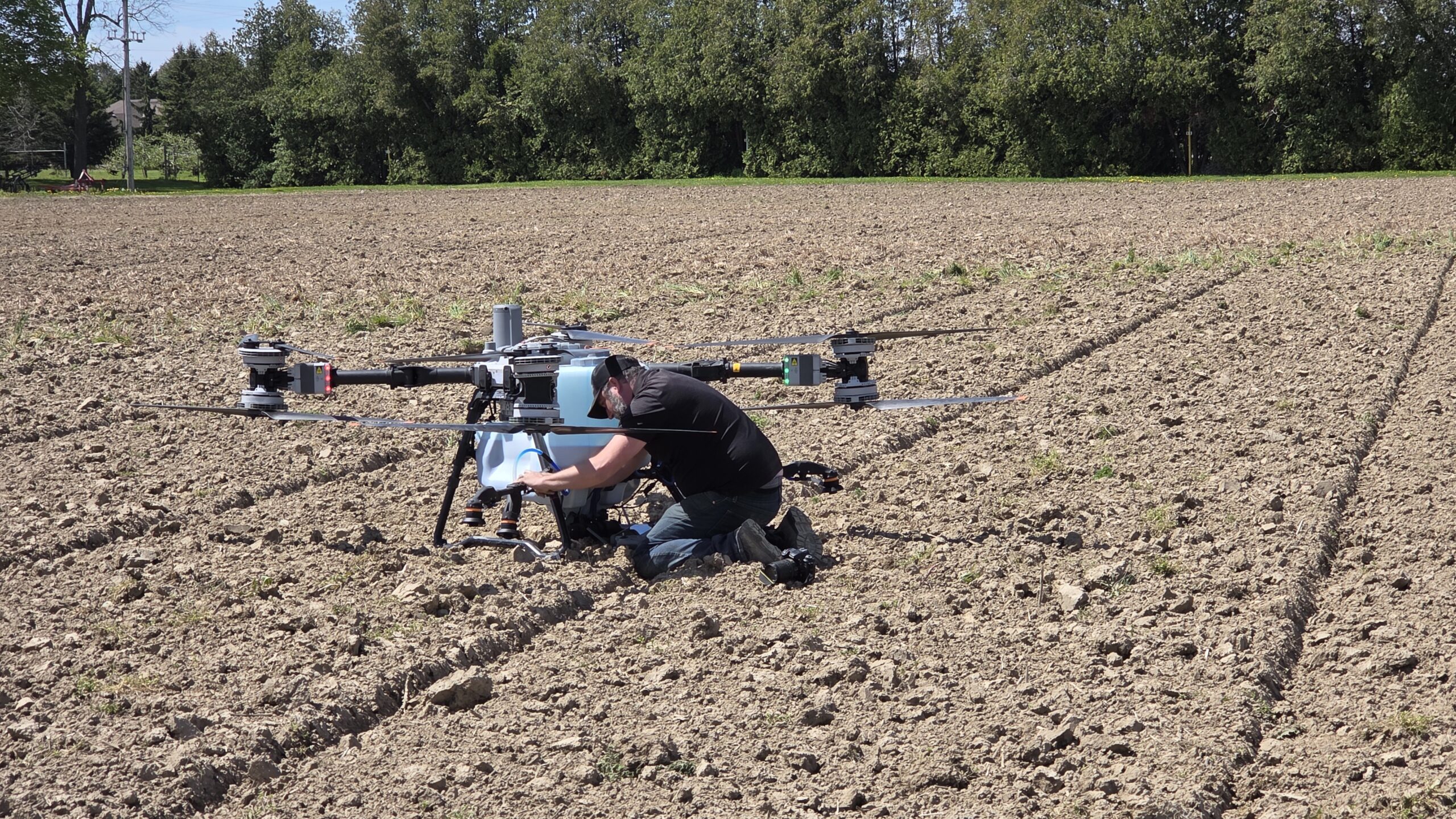
    The study was conducted at Ontario’s Simcoe Research Station on May 12, 2026. The site (42.857414, -80.271759) was a flat, recently tilled sand/loam field with no vegetation present. A DJI Agris T100 drone was used to perform the spray applications, supported by the D-RTK 3 relay station and flown on full auto.

    The spray mix was 0.2% v/v Super Signal Blue (Precision Laboratories) and 0.125% v/v Activate Plus NIS (Winfield United) in municipal water, pre-mixed to ensure consistency. A volume of 40 L – 60 L was maintained throughout the trial to minimize the effect of a changing payload.

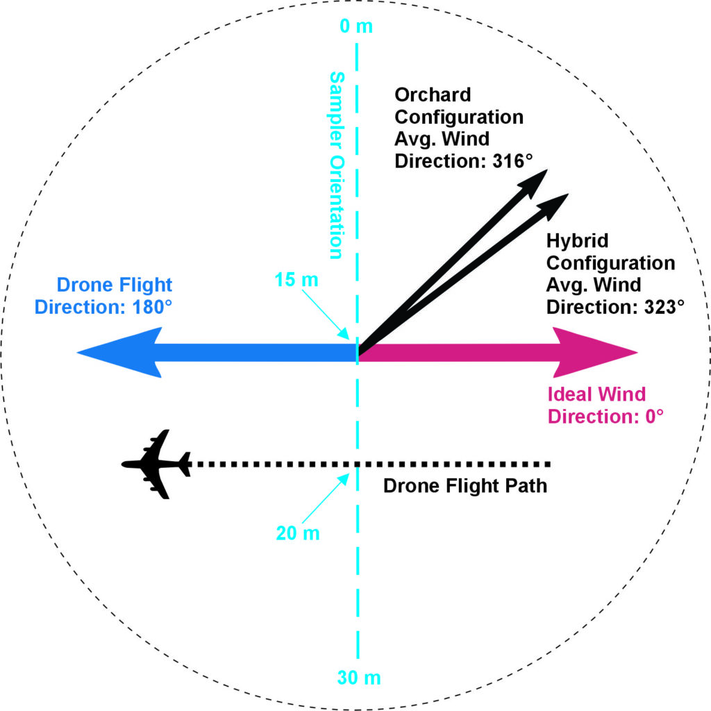
    The sampler was a flat, horizontal, continuous bond paper strip measuring 7.5 cm wide and 30 m long (secured in Speed Tracks™, Application Insight LLC). The sampler was oriented perpendicular to the prevailing wind, with the intention of flying the drone with a headwind across the 15 m mark (the centre) (Figure 2). Test passes determined that the T100 required 210 m to reach 20 m/s while half-full.

    Figure 2 – T100 spraying indicator dye across the 30 m continuous sampler.

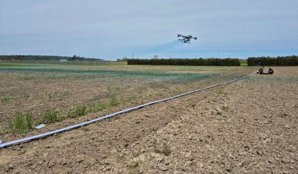
    Before the swathing runs began, the prevailing wind shifted direction slightly.  It was decided to fly the drone 5 m upwind (at the 20 m mark along the 30 m sampler) to ensure any downwind displacement was captured on the sampler (Figure 3).

    Figure 3 – Trial layout and prevailing wind conditions.

    Drone Settings and Swathing Order

    The primary objective of the study was to explore the effect of flight speed on swath width. Speed was increased from 8 m/s to the maximum 20 m/s by 2 m/s increments. Trial and error with the controller indicated that we could achieve these speeds by balancing an application volume of 30 L/ha and a programmed swath width of 7 m.

    Altitude was set to 4 m which is lower than the 5 m minimum recommended by DJI for high-speed flight. This was a compromise above the preferred 3.5 m altitude we have historically used with the T50. It was felt that higher altitudes would create unacceptable potential for swath displacement.

    Rotary atomizer design is not standardized, and as a result, the droplet size selected on the controller did not necessarily produce the desired results. The Hybrid configuration was programmed to emit 350 µm droplets, selected as a compromise between drift mitigation and coverage potential. To offset the Mister nozzles’ reputation for producing a finer spray, the Orchard configuration was set to the maximum 500 µm. Operations settings are noted in Table 1.

    ConfigurationNozzleDroplet size (µm)Speed (m/s)Altitude (m)Programmed Swath Width (m)Application Volume (L/ha)
    Hybrid4 Sprinklers3508, 10, 12, 14, 16, 18, 204730
    Orchard2 Misters, 2 Sprinklers5008, 10, 12, 14, 16, 18, 204730
    Table 1 – Operational settings for trials.

    Three repetitions of seven speeds were flown for each configuration. Anticipating an increase in temperature and wind speed throughout the day, it was decided move through all seven speeds (a single repetition) before resetting and doing so two more times. The intent was to preclude confounding weather effects. Ideally, we should have alternated between configurations as well, but this proved impractical. As a result, we flew the Hybrid configuration first and the Orchard configuration last.

    Weather

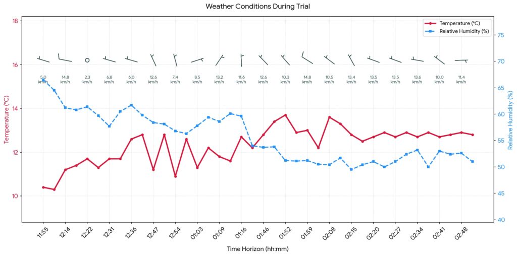
    Weather data was collected using a Kestrel 3550AG weather meter (Kestrel Instruments) in a vane mount positioned 2.5 m above ground. Temperature and relative humidity were comparable throughout the ~3 hours of data collection, but as anticipated, wind speed was higher for the later Orchard configuration passes.

    As previously indicated, wind direction shifted from an ideal headwind situation just before trials began, and was somewhat changeable, but the average wind direction for the two configurations was comparable (Figure 4 and Table 2).

    Figure 4 – Weather conditions recorded at roughly 10-minute intervals, corresponding to the drone passing over the sampler.
    TimeConfiguration FlownAverage Temperature (°C)Average Relative Humidity (%)Average Wind Speed (km/h ± SD)Average Direction (° ± SD)
    11:55 am – 1:16 pmHybrid11.759.98.4 ± 3.5323 ± 46
    1:43 pm – 2:52 pmOrchard12.951.611.9 ± 2.5316 ± 48
    Table 2 – Average weather conditions for the Hybrid configuration passes and for the Orchard configuration passes.

    Collector analysis

    Bond paper digitization

    Bond papers were scanned using a Swath Gobbler™ (Application Insight LLC). The software measured deposition as both percent area covered (% area) and deposit density (deposits/cm2) every 100 mm, with a thresholded Hue of 23-280, a Saturation of 5-120 and a Value of 156-255.

    Effective swath width calculation

    The large data set produced by each pass was reduced in size by avenging the deposition for every 50 cm. This data was entered into our Excel-based swath width calculator, which assumes a racetrack pattern and sums deposits from adjacent swaths. The resulting swath width for each pass was the maximum width that minimized over- and under-dosing as well as the coefficient of variation (CV).

    Analysis

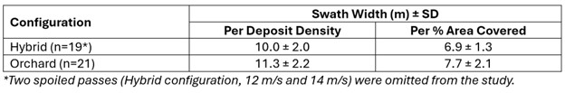
    The average swath width derived from deposit density data was wider than that derived from percent area covered (Table 3).

    Table 3 – Group means and standard deviation for average swath widths derived from deposit density data and percent coverage data. The average CV was between 29 and 32%.

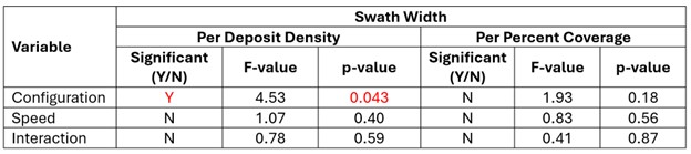
    A two-way ANOVA (Analysis of Variance; α = 0.05) was performed to determine any significant effect of speed or configuration on swath width (Table 4). Flight speed had no significant effect on swath width, no matter how it was derived (% area covered or deposit density), for either configuration (Hybrid or Orchard). However, the average swath width derived from deposit density was significantly wider for the Orchard configuration compared to the Hybrid and presented higher variability.

    Table 4 – Results of two-way ANOVA, exploring interactions between speed, swath width and configuration (95% confidence interval).

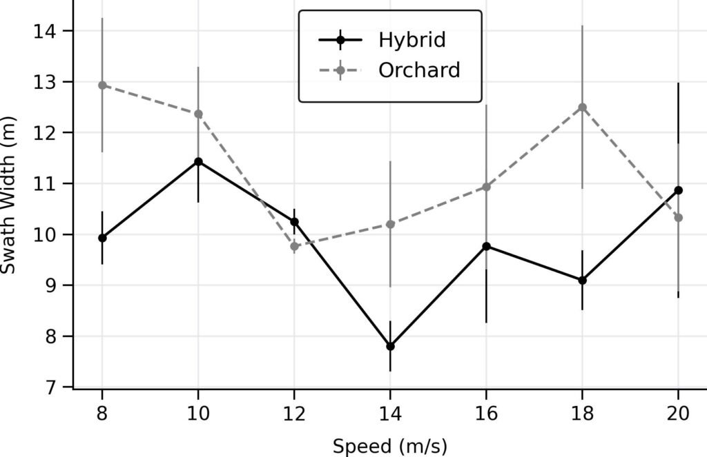
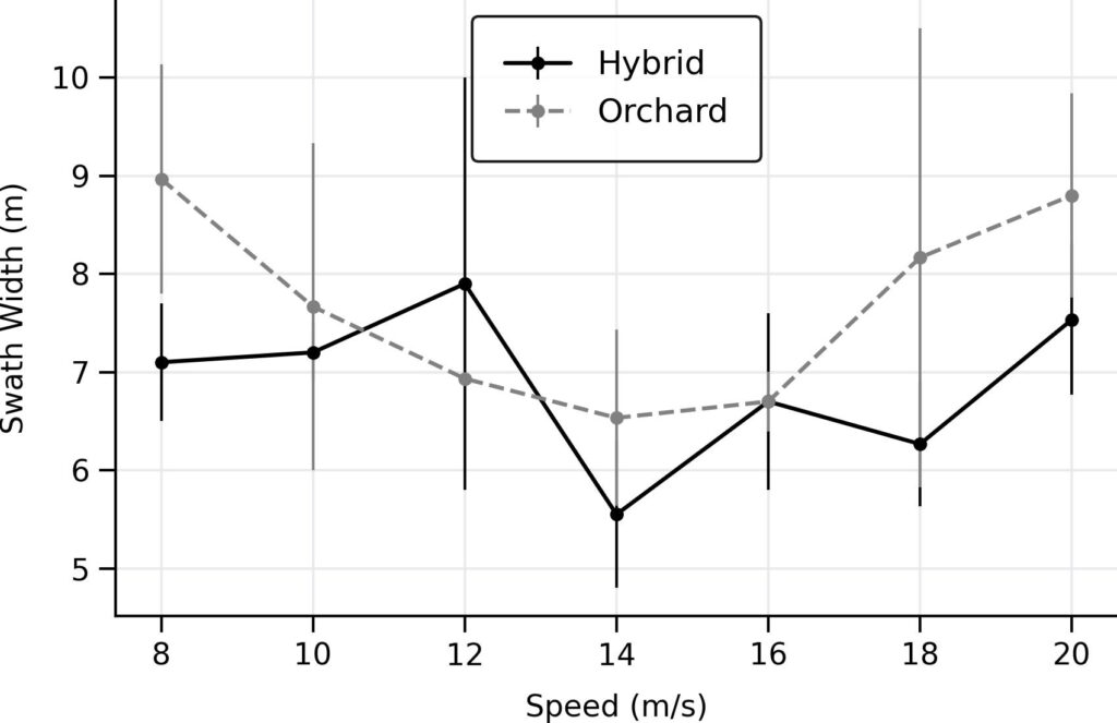
    Orchard configuration was prone to displacement in a side wind. Shifting the flight path 5 m upwind improved the downwind capture, but for some flights it did trim a small portion of the upwind deposition. Deposit density gives greater resolution and exposes more variability than percent area covered. Figure 5 shows the average deposition by speed based on deposit density. Figure 6 shows the average deposition by speed based on percent area covered.

    Figure 5 – Average deposition by speed based on deposit density. Arrow indicates flight path.
    Figure 6 – Average deposition by speed based on percent area covered. Arrow indicates flight path.

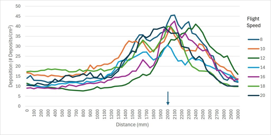
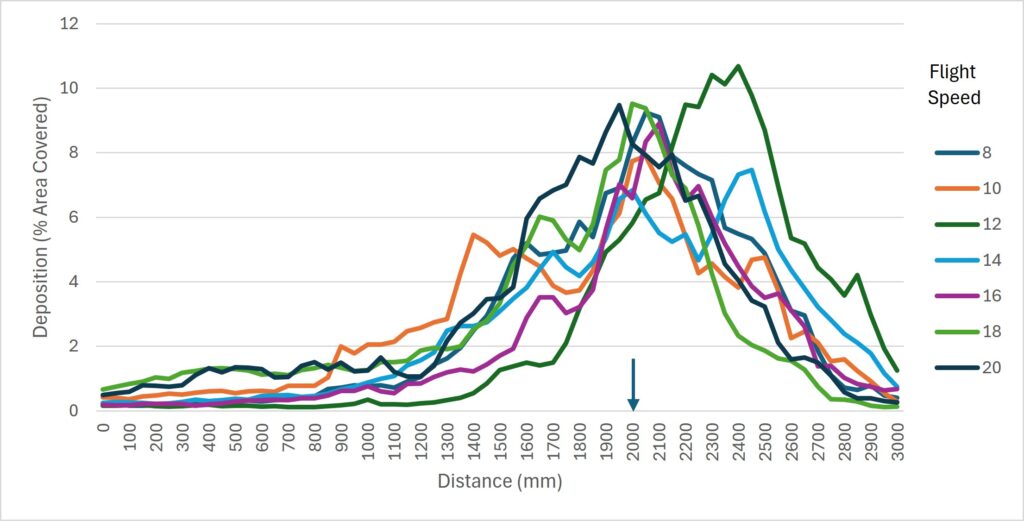
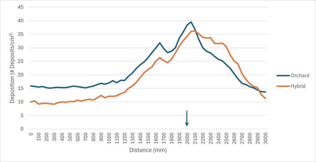
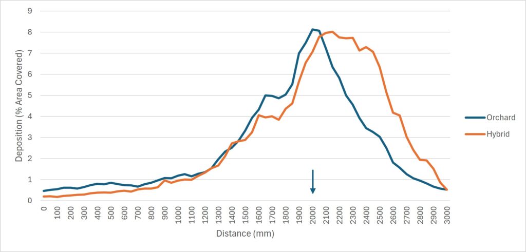
    Figure 7 shows the average deposition by configuration based on deposit density. Figure 8 shows the average deposition by configuration, based on percent area covered. Based on deposit density, there were 55% more deposits on the downwind side of the sampler for Orchard configuration set to set to 500 microns compared to the Modified configuration set to 350 microns.

    Figure 6 – Average deposition by configuration based on deposit density. Arrow indicates flight path.
    Figure 8 – Average deposition by configuration based on percent area covered. Arrow indicates flight path.

    The average swath widths calculated from percent area covered (Figure 9) and deposit density (Figure 10) are shown with standard deviation. While there appears the swath width is less around 14 m/s, it is statistically insignificant and the response to speed is essentially flat.

    Figure 9 – Average swath widths for each speed, derived from percent coverage data. SD shown. n=3 for each speed, while n=2 for Hybrid configuration at 12 m/s and 14 m/s.
    Figure 10 – Average swath widths for each speed, derived from deposit density data. SD shown. n=3 for each speed, while n=2 for Hybrid configuration at 12 m/s and 14 m/s.

    Observations

    Previous studies demonstrated a direct and positive relationship between drone speed and swath width up to 8-10 m/s. Here, we see no further response after ~8 m/s. This supports the hypothesis that rotary-wing drone speed and swath width share an asymptotic relationship that inflects at ~8-10 m/s. Variability makes it difficult to determine an exact value.

    Despite increasing the programmed droplet size to the maximum 500 microns for the Orchard condition, there was 55% more downwind deposition compared to the Hybrid condition, which was set to 350 microns. This supports the claim that the Mister nozzle produces a span of droplet sizes that include far more fines than the Sprinkler nozzle, and underpins the need for a better understanding of the spray quality produced by rotary atomizers.

    Spraying at high speeds is not an advisable practice. While swath width is no longer affected after ~8 m/s, there are other considerations. Note that it required 200 m for the drone to reach the highest speed, and in a related study we have seen swath width taper during initial acceleration and final deceleration, leaving gaps in coverage.

    Further, the minimum 5 m altitude advised by DJI ensures a safe margin for the drone to respond to obstacles and topography during high speed flight, but is not conducive to spraying. The author is aware of a situation where flying the T100 at 4 m altitude and 18 m/s over a canola field with rolling hills caused it to perform an emergency landing.

    An ideal speed is one that maintains the most consistent swath width at a reasonable altitude.

    Thanks to Drone Spray Canada and Bayer Canada for in kind and financial support, and thanks to Cesar Cappa, OMAFA horticulture weed specialist for his participation in the study.

  • Determining Airblast Travel Speed – The “Air Displacements” Method

    Determining Airblast Travel Speed – The “Air Displacements” Method

    The concept of Air Displacements was developed by Dr. David Manktelow, Applied Research and Technologies Ltd.

    What is the “right” speed to drive when spraying?

    Airblast sprayer operators must know their average travel speed to calculate how much pesticide and time is required to complete a spray job. Note that it’s an average, not a constant, because travel speed is significantly affected by ground surface conditions (e.g. slippage), grade (e.g. hills) and the weight of the rig (e.g. as spray mix is depleted).

    The pursuit of productivity and the unchallenged status quo of traditional spray volumes, blinds many operators to the fact that travel speed is a critical factor in focusing air energy on the target canopy. As long as droplets are small enough to be entrained and directed by the air, we believe that optimizing the fit between air energy and the target canopy leads to the most frugal and effective use of spray mix and should therefore dictate travel speed. If that speed proves to be painfully slow, or terrifyingly fast, then a mismatch is revealed between the sprayer design and the operational conditions and the overall spraying strategy should be reconsidered.

    This article describes a method for modelling an ideal travel speed. It can be used as a sanity check for existing operations or for those seeking to evaluate the fit of a new airblast sprayer. However, this method can only approximate travel speed. A true optimization of sprayer settings will require fine tuning using the ribbon method and, ultimately, coverage feedback from water sensitive paper (see here and an older article here). We’ll begin with how to measure average travel speed.

    How to measure average travel speed

    Beware the tractor speedometer or rate controller that monitors wheel rotations; both can be fooled by changes in wheel size, tire wear or slippage. GPS or radar-based speed sensors are the most accurate method.

    Those that prefer a manual method can follow this classic protocol for determining average travel speed:

    1. Go to a row that is representative of the terrain in your planting. Measure out a distance of 50 m (150 ft) and mark the start and finish positions with wire marker flags.
    2. Fill the sprayer tank half full of water.
    3. Select the gear and engine speed in which you intend to spray. If using a pull-behind sprayer, ensure the PTO is running or you could introduce errors.
    4. Bring the sprayer up to speed for a running start and begin timing as the front wheel passes the first flag. This is far easier when there are two people.
    5. Stop the timer as the front wheel passes the second flag.
    6. Stay out of any ruts and run the course two more times.
    7. Determine the average drive time for the three runs (i.e. the sum of all three times in seconds divided by three).
    8. Finally, calculate travel speed using one of the following formulae, depending on preferred units:

    Ground Speed (km/h) = Average drive time for 50 m (s) ÷ 13.9 (a constant)

    Those that prefer a less accurate but convenient hack can download any smartphone speedometer app that can calculate an average (similar to a runner’s GPS wristwatch). Fill the sprayer tank half full and drive a representative section of your operation with the fan on and the spray off. Consult the phone for your average speed for each pass. Take a screen shot and email it to yourself as a time-stamped component of your spray records.

    The “Air Displacements” method

    Dwell time

    Airblast sprayers use fans to move a volume of air at a certain speed, often measured in m3/hr or ft3/min. Imagine that volume of air as a three dimensional shape extending from the air outlet over a distance. Likewise, imagine the void between the sprayer outlet and the target canopy as a three dimensional shape penetrating roughly halfway into that canopy (assuming we intend to spray every row).

    How long must the sprayer dwell in one spot before it pushes all the intervening air out of the way and replaces it with spray-laden air? If the sprayer drives too slowly, it will wastefully push spray through and beyond the target (i.e. blow-through). If the sprayer moves too quickly, the spray will not have an opportunity to penetrate the target canopy and most certainly not reach the highest point. This concept of focusing air energy using travel speed is called Dwell Time.

    We want to calculate the volume of air the sprayer generates, compare that to the volume we want displaced, and then determine how fast we must drive to optimize the fit. We can do all this with a tape measure, an anemometer, and a partner to record the data and do a little math.

    1. Measure air outlet area

    With the sprayer safely off, measure the area of the air outlet(s) on one side of the sprayer. We’ll use a Turbomist 30P Low Drift Tower (below) as an example. There are two air outlets that are 5 cm wide by 150 cm high for a total area of 0.075 m2 on each side. Be sure to look inside the outlet for any irregularities like baffles or obstructions intended to block air. Subtract those areas from the total. Don’t worry about small things like nozzle bodies.

    For rectilinear outlets: Height (m) x width (m) = Area (m2)

    For circular outlets: 3.14 x radius2 (m) = Area (m2)

    The air outlet on this Turbomist 30P Low Drift tower sprayer is 5 cm wide by 150 cm tall for a total area of 0.075 m2.

    2. Measure air speed

    First, a few safety warnings: High speed air is loud and can carry debris, so always wear ear and eye protection and respect the hazards inherent to working with air-assist sprayers. Only use an anemometer rated for at least 160 km/h (100 mph) (e.g. here). Do not use a handheld weather meter such as a Kestrel because the impellor could be destroyed and become dangerous shrapnel.

    Use an anemometer rated for at least 160 km/h (100 mph) (e.g. here). Do not use a handheld weather meter such as a Kestrel because the impellor could be destroyed and become dangerous shrapnel.

    Bring the fan up to speed and holding the meter about 25 cm (10 in.) from the outlet, measure the air speed at several locations along the air outlet both vertically and horizontally. We calculate an average speed because many air outlets do not produce uniform air speed or volume along their outlets. For this example, we measured four locations along the air outlet on both sides of the sprayer and saw significant differences. We did this both in low and high gear (see table below).

    High GearHigh GearLow GearLow Gear
    Location Along OutletLeft Side (m/s)Right Side (m/s)Left Side (m/s)Right Side (m/s)
    Top 1/441.180.342.924.6
    Upper34.932.226.430.8
    Lower30.830.024.026.4
    Bottom 1/433.540.226.831.3
    Average35.145.730.028.3
    Anemometer readings from the low drift tower sprayer outlets, on left and right side, in high and low fan gear. Four readings from bottom to top to determine the average. Readings taken 25 cm from edge of outlet and PTO set to 540 rpm.

    Multiple air outlets

    Before we continue with the method, let’s change sprayers to this Turbomist 30P Grape Tower (below). The design is intended to spray adjacent rows from the vertical outlets (5 cm x 150 cm = 0.075 m2) along the tower. The upper, inverted outlets (10 cm x 63.5 cm = 0.0635m2) throw spray over the adjacent rows and cover the outside rows. The intention is to improve productivity by covering four rows of grape (or possibly three) per pass.

    The Turbomist 30P Grape Tower Sprayer is a multirow system intended to drive every third or fourth row.
    Lower, vertical ducts are 5 cm x 150 cm = 0.075 m2
    Upper, inverted ducts are 10 cm x 63.5 cm = 0.0635m2

    However, when we consider this design through the Air Displacement lens, it’s almost like having two sprayers performing two jobs simultaneously. The vertical outlets and the upper, inverted outlets are different shapes. Further, their position (distance and angle, as the top outlets are angled back more aggressively) relative to their respective target canopies are significantly different. How fast must this sprayer drive to optimize the fit? Do we have to compromise coverage and incur drift and waste from one set of outlets to accommodate the other set? The manufacturer has worked to address this potential issue by partitioning the majority of the air energy to the top outlets, but let’s see how that affects travel speed.

    3. Total volumetric flow

    Having already measured the outlet area, we then measured average air speed (see table below).

    High GearHigh GearLow GearLow Gear
    Location Along OutletLeft Side (m/s)Right Side (m/s)Left Side (m/s)Right Side (m/s)
    Top Outlet27.026.527.026.0
    Bottom Outlet12.013.010.512.5
    Average anemometer readings (n=4) for top and bottom outlets, on left and right side, in high and low fan gear. Readings taken 25 cm from edge of outlet and PTO set to 540 rpm.

    Now we can use these two values to determine how much air the sprayer generates by calculating total volumetric flow. We first have to convert air speed from m/s to m/h to make the units work, so just multiply it by 3,600. Then we multiply that by the outlet area and we get the table below.

    Average air speed (m/s) x 3,600 (a constant) = Average air speed (m/h)

    Average air speed (m/h) x Outlet area (m2) = Total volumetric flow (m3/h)

    High GearHigh GearLow GearLow Gear
    Location Along OutletLeft Side (m3/h)Right Side (m3/h)Left Side (m3/h)Right Side (m3/h)
    Top Outlet6,172.06,058.06,172.05,944.0
    Bottom Outlet3,240.03,510.02,835.03,375.0
    Total volumetric flow for top and bottom outlets, on left and right side, in high and low fan gear, with PTO at 540 rpm.

    4. Target volume to displace

    Now that we know the volume of air the sprayer generates, let’s determine the volume of air we need to replace with that spray laden air. This is really the only tricky bit because you have to picture a cross section and then measure the shape. See the illustration below.

    For the bottom outlet, it’s simple. The outlet is 81 cm from the grape panel and the grape panel is 112 cm high. We calculate the area of a rectangle by multiplying length by width, so:

    Length (cm) x Width (cm) = Area (cm2)

    However, the sprayer design makes the top outlet’s job trickier to figure out. This isn’t a rectangle, it’s a “quadrilateral”. We get this odd shape when either the sprayer outlet or the target canopy are significantly taller than the other. Fortunately this one has a right angle so we don’t have to brush off our high school trigonometry textbooks. Instead, we can lean on the internet using this link and plug in the values. As we can see below, the cross sectional areas spanning from the outlets and the middle of the target canopies are 0.9 m2 for the bottom outlet, and 2.35 m2 for the upper outlets.

    This gives us a cross sectional area, but we need to convert that to a volume so we can compare the air generated to the air needed. To do that, we multiply the cross sectional area by 100 m, representing how much air would be needed over 100 m of row length. The formula and the results are presented below.

    Cross sectional area (m2) x 100 m of row length = Target displacement volume (m3)

    OutletTarget Displacement Volume (m3)
    Top Outlet235.0
    Bottom Outlet90.0
    Target displacement volume for each outlet over 100 m of canopy row.

    5. Displacement rate

    We see the target displacement volumes for each outlet are significantly different. Assuming the air from the upper outlet maintains its integrity and reaches its target canopy without being blown off course, it must produce enough air energy to fill more than twice the displacement volume of the lower outlet. We can see from the earlier calculations that it does produce almost twice the total volumetric flow. But is it enough? To know we must calculate the Displacement Rate for each outlet. Let’s just focus on the left side of the sprayer in high gear.

    Total volumetric flow (m3/h) ÷ Target Volume (m3) = Displacement Rate ( displacements/h)

    OutletDisplacement Rate (displacements/h) for left side of sprayer in high gear
    Top Outlet26.25
    Bottom Outlet36.0
    Displacement rates for the outlets on the left side of the sprayer in high gear.

    So we see that the outlets at the top of the sprayer, if stationary, could displace the target volume of air 26.25 times an hour. However, the lower outlet would displace its target volume 36 times in that same hour. We see that we might have a problem. But this is for a stationary sprayer and not a sprayer in motion. The last step gives us what we came here for.

    6. Ideal travel speed

    We can now determine the ideal travel speed for this sprayer using that same 100 m row length.

    [Displacement rate (displacements/h) x 100 m of row length] ÷ 1,000 (a constant) = Ideal travel speed (km/h)

    OutletIdeal travel speed (km/h) based on left side of sprayer
    Top Outlet2.6
    Bottom Outlet3.6
    Ideal travel speed for each outlet on the left side of the sprayer in high gear.

    As we stated at the beginning of this article, this is only a model. It doesn’t account for canopy density and assumes the spray laden volume of air produced by the sprayer can reach the target intact over a given distance. However it does indicate that there is a potential issue that will lead to either over spraying the adjacent row (slower travel speed) or under spraying the distant rows (faster travel speed) which could lead to waste, drift and poor coverage.

    In the image below, we chose to drive close to 2.6 km/h in high gear. No effort was made to adjust the liquid flow (i.e. change the nozzles) so there was too much spray volume here, but we can see the losses on the left (upwind) side, and the blow-through three rows over on the right (downwind) side. Leaving aside the excessive liquid volume, we could drive faster or reduce the fan gear to reduce the blow-through on the adjacent rows, but we may go too fast (or reduce the rate of air displacement) for the upper outlets to reach the target. We can already see the integrity of the upper-left outlet breaking down as it sprays into the wind.

    Testing a travel speed. No effort was made to adjust liquid flow, which is excessive here. Cross wind was from the left to the right in the image. Photo by Corey Parker (Instagram: _parkerproductions)

    Take home

    An ideal travel speed for an airblast sprayer is more than just being productive. The spray must reach and penetrate the target. If this requires dangerously high speeds, or if you simply can’t move slowly enough, it suggests a problem with the spraying strategy. Changes will have to be made to the sprayer, the target canopy, or even the weather conditions you’re willing to spray in. Getting the job done quickly should not compromise the quality of the job. Use this method to re-evaluate your practices, or to assess the capabilities of candidate sprayers if you’re considering a new purchase. Be sure to confirm what this model is telling you using some coverage indicator, such as water sensitive paper.

    Happy spraying.

  • Gear up – Throttle down

    Gear up – Throttle down

    In 1977, David Shelton and Kenneth Von Bargen (University of Nebraska) published an article called “10-1977 CC279 Gear Up – Throttle Down”. It described the merits of reducing tractor rpm’s for trailed implements that didn’t need 540 rpm to operate. In 2001 (republished in 2009), Robert Grisso (Extension Engineer with Virginia Cooperative Extension) described the same fuel-saving practice. Again, it was noted that many PTO-driven farm implements don’t need full tractor power, so why waste the fuel? He tested shifting to a higher tractor gear and slowing engine speed to maintain the desired ground speed. 700 diesel tractors were tested, and as long as the equipment could operate at a lower PTO speed and the tractor itself didn’t lug (i.e. overload), as much as 40% of the diesel was saved.

    How this applies to Airblast

    For airblast operators with PTO-driven sprayers and positive-displacement pumps, this has potential for reducing air energy. Gearing up and throttling down (GUTD) sees the operator reducing the PTO speed from 540 rpm to somewhere between 350-375 rpms, which not only saves fuel but more importantly slows the fan speed. This may be an option when air energy from the sprayer, even at higher travel speeds and a low fan gear, still overblows the target canopy.

    Some airblast sprayers, like this one, feature fan blades with adjustable pitch to increase or lower air volume and speed. It’s often a pain to try to adjust them, and most operators only try it once.
    Some airblast sprayers, like this one, feature fan blades with manually-adjustable pitch to increase or lower air volume and speed. It’s often a pain to try to adjust them, and most operators only try it once.

    A good time to try this out is early in the spraying season when (most) canopies are dormant and at their most sparse. For example, when applying dormant sprays in apple orchards, look to see if the wood on the sprayer-side gets wet, but does not creep around the sides. This suggests that the air, and much of it’s droplet payload, are being deflected. When the air speed is slowed, it will become more diffuse and turbulent on target surfaces, and this turbulence helps more droplets deposit in a panoramic fashion within (not past) the target canopy. Look to see if the wood is wet >50% around the circumference of the branches. You’ll get the rest when you spray form the other side.

    Limitations

    GUTD is not always appropriate. It requires airblast sprayers with PTO-driven positive displacement pumps (e.g. diaphragm). Airblast sprayers with centrifugal pumps would experience a drop in operating pressure and would have to be re-nozzled. Further, the pump must have sufficient surplus capacity to maintain pressure at low rpms.

    GUTD is not intended for air-shear sprayers that employ twin-fluid nozzles because dropping air speed below a certain threshold may compromise spray quality; the air needs to be fast enough to create and direct spray droplets

    The tractor must have sufficient horsepower (more than 25% in excess of minimally-required capacity) to permit the reduction in engine torque. This is especially important if the operator is on hilly terrain. If the tractor begins to lug (e.g. black smoke, sluggish response, strange sounds) you’ll be in trouble.

    Observations

    We first experimented with GUTD in 2013. We noticed how much quieter the sprayer was, and the fuel consumption was certainly reduced. One grower-cooperator switched to a GUTD spray strategy mid-way through their dormant oil application in pears. We saw the trees immediately began to drip. Panoramic coverage was improved significantly; once the operator passed down the other side of the target, capillary action and surface tension helped to give near-complete coverage.

    However, in one instance, the operator was already applying a low spray volume per hectare using air induction nozzles and their lowest fan gear. By further slowing fan speed using GUTD, coverage at the top of his cherry trees was compromised.

    In short, GUTD can work under the right circumstances. If you want to try it, use water-sensitive paper to establish a base-line with your current practice, and then evaluate coverage after you change your sprayer settings.

  • How to Size a Nozzle for Pulse Width Modulation (PWM)

    How to Size a Nozzle for Pulse Width Modulation (PWM)

    PWM is gaining popularity, and there is an ever-increasing number of first-time users that need to make nozzle selections for their system. We’ve written about it here, here, and here.

    Recall the PWM replaces spray pressure with Duty Cycle (DC) of a pulsing solenoid as the primary means of controlling nozzle flow. The solenoid shuts off the flow to the nozzle intermittently, between 10 and 100 times per second depending on the system. The Duty Cycle is defined as the proportion of time that the solenoid is open, and for low-frequency systems, DC is more or less linearly related to flow rate.

    The first rule of PWM nozzle selection is to understand that under average travel speeds, we’d like to see the duty cycle of the system at between 60 and 80%. This means that the nozzle solenoid is open about 2/3 of the time. This value also describes the flow rate as a proportion of the full capacity that nozzle.

    The reason for this 2/3 duty cycle rule is to enable four key features of PWM:

    1. It’s ideal for turn compensation, allowing the outer nozzles to increase their flow 20 to 40%, and the inner nozzles to decrease flow about three-fold, in accordance with boom speed.
    2. It allows speed flexibility, providing some additional speed, but more importantly, reduced speeds should conditions require it, without a change in spray pressure.
    3. It compensates for pressure changes so that spray quality can be adjusted without requiring a speed change. Less pressure reduces nozzle flow, and increasing DC recoups accordingly.
    4. It allows for customized higher flows of certain nozzles, perhaps behind wheels, to address reduced deposition in their aerodynamic wake (available on some PWM systems).

    The best tool for selecting the right nozzle size is Wilger’s Tip Wizard. This site asks for your desired average speed ( although it calls this “Max Sprayer Speed”), and reports the expected DC for a host of nozzle size solutions and pressures. It also reports maximum and minimum travel speeds and other useful information such as spray quality.

    Fig 1: The Tip Wizard is a useful tool for sizing nozzles on any PWM system. Sizing information applies to any nozzle. Spray quality information is for Wilger ComboJet nozzles only.

    Although intended for Wilger nozzles, the site’s sizing feature works for any nozzle brand. It asks the user which PWM system they have for the purpose of calculating the documented pressure drop across the solenoid.

    Fig 2: Tip Wizard results for the Wilger SR11006 tip at 10 gpa and 15 mph. Look for a solution that provides 60 to 80% Duty Cycle (DC).

    If you don’t have access to the site, a basic calibration chart can still work with a simple trick. Recall that we use the top row to identify the desired water volume, and the table’s interior values are speeds, as described here.

    Below are two solutions for someone wanting to apply 10 gpa at 15 mph without PWM. The correct choice depends on the required pressure to produce the needed spray quality.

    Fig 3: A conventional calibration chart, solving a 10 gpa application for 15 mph.

    If you want to apply the same 10 US gpa using PWM, simply solve for a larger volume that offers the right DC. For example, choosing 13 gpa will over-apply by 3 gpa, or 30%. The PWM system adjusts by running at 100-30=70% DC. If the chart doesn’t offer 13 gpa, go nearby, to 14 gpa, as we did below:

    Fig 4: By pretending to require 14 gpa instead of the actual 10 gpa, the conventional calibration chart is tricked into solving for a nozzle size that will work with PWM at 60% Duty Cycle.

    Now solve for the same target speed, 15 mph. The solution will run at 60% DC. Again, there is more than one choice, and that will depend on the spray pressure needed.

    Fig 5: Two possible solutions for achieving 10 gpa at 10 mph. An 06 nozzle at intermediate pressure or an 08 nozzle at low pressure.

    We’ve developed a template, in US or metric units, that can be customized for any water volume. Here is the same chart with 13 gpa added:

    Fig 6: A conventional calibration chart with the 13 mph speed added.

    The best solution for 10 gpa at 15 mph is the 06 size nozzle at 50 psi. This is not engraved in stone. One of the nice things about PWM is that it has inherent flexibility. Make the nozzle pressure a priority to get the correct spray quality. It really doesn’t matter whether the resulting DC is 65 or 80%, the system will still work well. Simply avoid extremes that take you below 50% or above 90%, they will limit the system’s capabilities.

    The worksheet can be downloaded below:

    It can handle any water volume or nozzle spacing by filling in the blue cells. Two additional worksheets in the file automate the process, simply enter the desired application volume, travel speed, and nozzle spacing (yellow cells), and the solution that offers the optimal duty cycle range will be highlighted in light green.

  • Exploding Sprayer Myths (ep.4): Speed Spraying

    Exploding Sprayer Myths (ep.4): Speed Spraying

    All set for Star Wars VII
    All set for Star Wars VII

    With due respect to Mickey and Mr. Lucas, and the massive hype surrounding Star Wars Episode VII, we felt we should jump on the bandwagon. Here’s episode IV in our series of short, educational and irreverent videos made with Real Agriculture.

    If there’s a single take-home message in this episode it’s this:

    …may the force be with you – always.