This 2023 article is based on work performed by Mike Schryver, BASF Technical Service Specialist.
Nitrogen is an essential nutrient required throughout a plant’s lifecycle. It is commonly applied to corn in either a granular form as urea or in a liquid form as urea-ammonium nitrate (UAN). Depending on soil type and precipitation, significant amounts of nitrogen can be lost to leaching, denitrification and volatilization as N2O (a greenhouse gas). Learn more about nitrogen in soil in this excellent overview by University of Minnesota Extension.
With the 2020 announcement of Canada’s Strengthened Climate Plan, Ontario is committed to a 30% reduction of 2020 N2O emission levels by 2030. Adding urease and nitrification inhibitors (aka stabilizers) to nitrogen fertilizer applications is an environmentally sustainable practice that reduces nitrogen losses and improves yield.
Another essential plant nutrient, Sulphur, is applied in liquid-form as ammonium thiosulphate (ATS). Primarily used to increase corn yields, high rates (approx. >10% by volume) of ATS can also inhibit urease and nitrification, albeit not as well as other nitrogen stabilizing options.
In the pursuit of productivity, UAN and ATS are often combined to serve as an herbicide carrier in corn weed-and-feed applications. However, liquid fertilizers are dense solutions that contain charged ions and exhibit a reduced capacity for solubilizing pesticides. This complicates the tank mixing process. When micronutrients like sulfur are added to nitrogen-based formulations, physical incompatibilities can arise that cause uneven applications and can even clog sprayers.
Given the known compatibility issues, questions have been raised about the best way to introduce urease and nitrification inhibitors to tank mixes of UAN, ATS and herbicide. Specifically:
Stabilizer Compatibility: What is the impact of adding nitrogen stabilizers to UAN carriers containing leading corn herbicides formulated as emulsifiable concentrates (EC) or suspension concentrates (SC)?
Mixing Order: When UAN and ATS are premixed, does their ratio, or the addition of nitrogen stabilizer affect tank mix compatibility with herbicides?
To answer these questions, we performed a series of jar tests.
Method
300 ml jars with magnetic stir bars were mixed to reflect a 10 gpa application. UAN was chilled to approx. -5°C and herbicides were added at 2x the labelled rate to simulate a worse-case scenario. Nitrogen stabilizer was added at a ratio per manufacturer’s instructions. Products were introduced at 1 minute intervals to provide sufficient time for solubilization. Jars were left to rest for at least 1 hour after mixing, and then agitated to simulate interrupted spray jobs. The solution was then poured through a 100 mesh screen to simulate a worst case scenario for sprayers that typical employ 50 mesh filters.
Herbicides
Fertilizer carriers
Stabilizers
Leading EC Herbicide
UAN: 28%
eNtrench NXTGEN (Corteva)
Leading SC Herbicide
ATS: 12-0-0-26% SU
Anvol (Koch)
Tribune (Koch)
Agrotain (Koch)
Neon Surface (NexusBioAg)
SylLock plus (Sylvite)
Excelis Maxx (Timac)
Table 1 Herbicides, carriers and stabilizers used in the study
Results
Stabilizer Compatibility
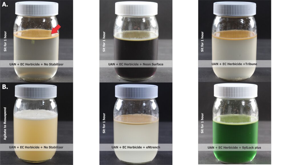
EC herbicides have active ingredients that are soluble in water and include immiscible solvents. When added at 2x label rate to chilled UAN, followed by a stabilizer, agitation created an acceptable suspension (Figure 1). The EC separated to the top of the mixture following an hour rest but was easily reintegrated. There was no appreciable residue left behind when poured through a 100 mesh screen.
Figure 1 UAN + EC Herbicide + Stabilizer after 1 hour rest. Image A is a control with no stabilizer and image B is the same control after agitation. The arrow indicates where ECs separate at the top of each jar. All products resuspended with agitation.
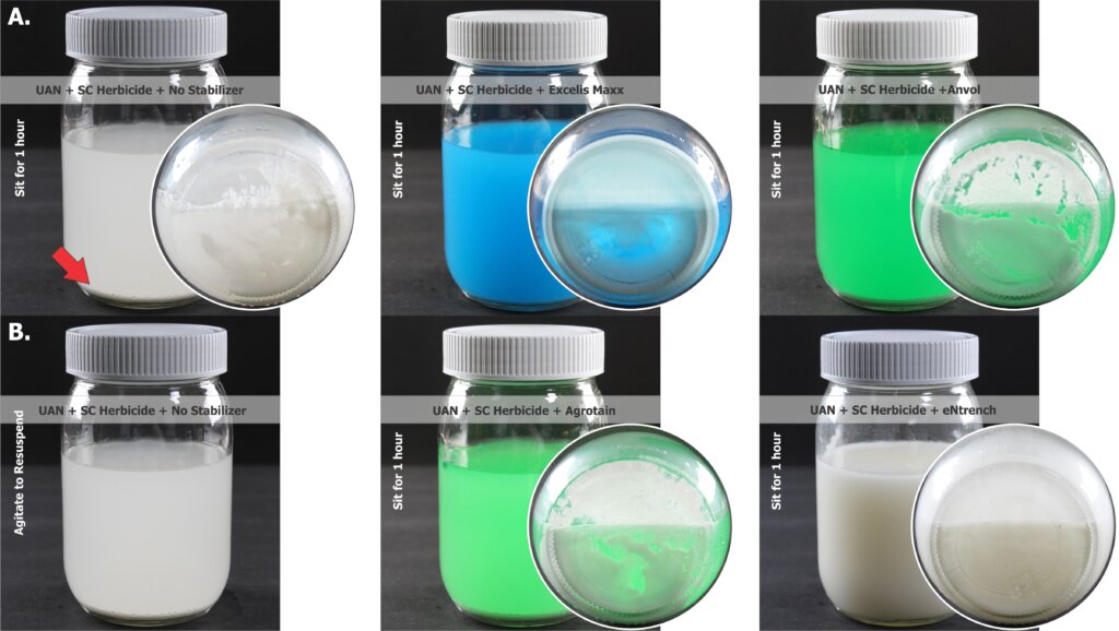
SC herbicides have active ingredients that are water insoluble, but stable in an aqueous environment. When added at 2x label rate to chilled UAN, followed by a stabilizer, agitation created an acceptable suspension (Figure 2). The SC flocculated and formed a sediment at the bottom of the mixture following an hour rest but was easily reintegrated. There was no appreciable residue left behind when poured through a 100 mesh screen.
Figure 2 UAN + SC Herbicide + Stabilizer after 1 hour rest. Image A is control with no stabilizer and image B is the same control after agitation. The arrow indicates where SCs settled, as depicted in the inset images showing the bottoms of each jar. All products resuspended with agitation.
Best Practices
Contact manufacturers and conduct a jar test to confirm compatibility
Ensure thorough agitation (with or without a stabilizer, and especially after tank has settled)
Components may separate to the top (ECs) or settle on the bottom (SCs)
Mixing Order
Mixing order was tested using chilled UAN, ATS, and EC herbicide. It is well known that ATS should be added last in the tank mix order, and mixes that include a higher load of ATS relative to UAN exacerbate tank mix issues.
This is seen in the following video where we combine 203 ml of chilled UAN, 30 ml of SC corn herbicide and 68 ml of ATS. On the left, UAN, then herbicide, then ATS mixes perfectly. However, when we start with UAN, then add ATS (which represents premixed fertilizer) then the herbicide does not suspend, and prolonged agitation does not improve the situation. The video is shown at 2x speed.
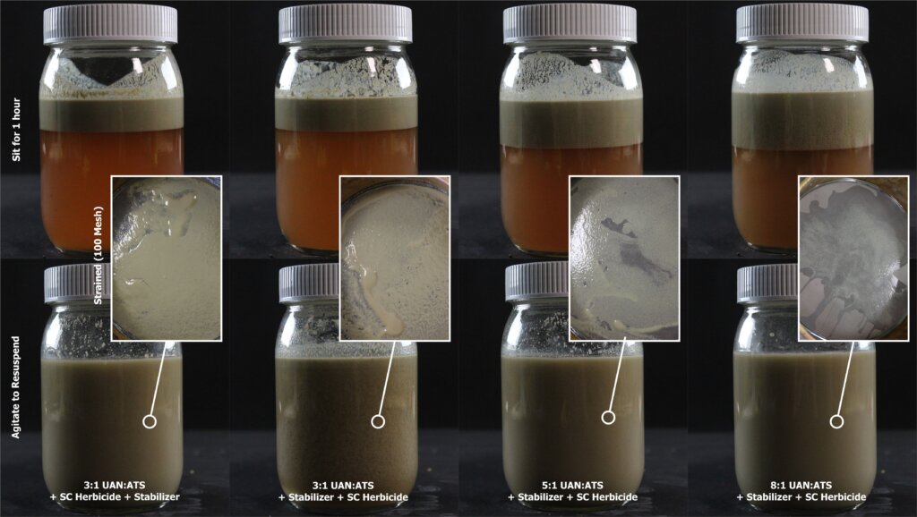
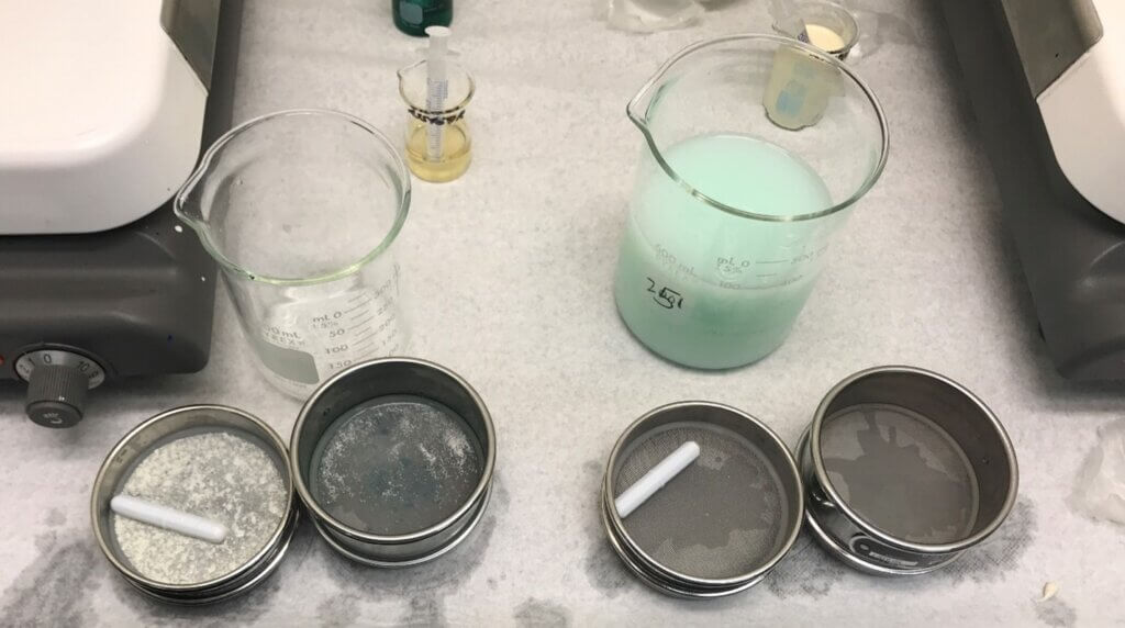
We then added a nitrogen stabilizer to the series to see if it could correct the tank mix issue arising from adding ATS immediately after UAN. This replicates the situation an operator would face when purchasing UAN and ATS premixed. We also reduced the ratio of UAN to ATS from 3:1, to 5:1 to 8:1 to establish a threshold ratio that alleviated tank mix issues (Figure 3). All solutions were poured through 100 mesh screens to capture residue (Figure 4).
Figure 3 SC Herbicide and stabilizer added to UAN and ATS premixed at different ratios. Agitated after 1 hour and poured through 100 mesh screens (inset images).Figure 4 Pouring EC jar test solutions through 100 mesh screens
Best Practices
Contact manufacturers and conduct a jar test to confirm compatibility
ATS must be added after the herbicide (EC or SC). The stabilizer can be added last, but preferably ATS is the last ingredient in the tank.
Adding stabilizer will not reverse a tank mix error arising from adding ATS prior to the herbicide.
The higher the concentration of ATS, the higher the risk of incompatibility. A 5:1 ratio of UAN to ATS failed while a ratio of 8:1 succeeded. The threshold is likely 7:1.
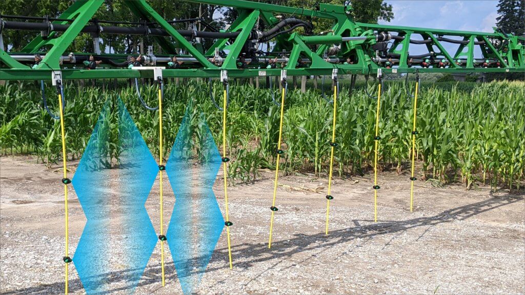
In 2019 we evaluated the spray coverage from nine application methods on corn silks. The results showed that a directed application from drop hoses (aka drop pipes, drop legs) suspended in between the rows gave significantly higher deposits. The results led us to wonder if the superior coverage from a directed application translated to improved yield.
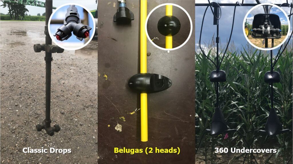
Around this time we started considering the Beluga Drop Hose developed by Agrotop (Germany) and distributed by Greenleaf Technologies (USA). Originally designed to apply neonicotinoids in canola, we found that the stiff-but-flexible hose did not tend to deflect or sway during an application. Further, their unique low-profile nozzle body had less potential to cause mechanical damage or otherwise snag in dense canopies. Unlike homemade drop pipes or other commercial solutions such as the Y-Drop with 360 Undercover, the Belugas were lightweight, simple to install/remove, and did not need a break-away section to prevent damage.
Three examples of directed application systems. Left: Homemade drop pipes and a TeeJet QJ90-2-NYR split nozzle body (inset). Centre: Beluga drop hose with streamlined nozzle body (inset). Right: Y-Drop side-dress drop pipes with Yield 360 Undercover option (inset).
In 2021 we initiated a four-year trial with the Beluga drop hose system in Port Rowan, Ontario. Our objective was to evaluate return-on-investment based on yield using two pesticide regimes. Treatments were established for conventional overhead technology, directed applications (i.e. the Beluga) and unsprayed checks.
Construction and Installation
We ordered 150 cm (60″) drop hoses with two nozzle bodies each so we could customize them. The instructions were in German, but after running them through translation software we were confident in how to proceed (download the translated copy here). We started by determining the hose length.
Hose Length and Boom Spacing
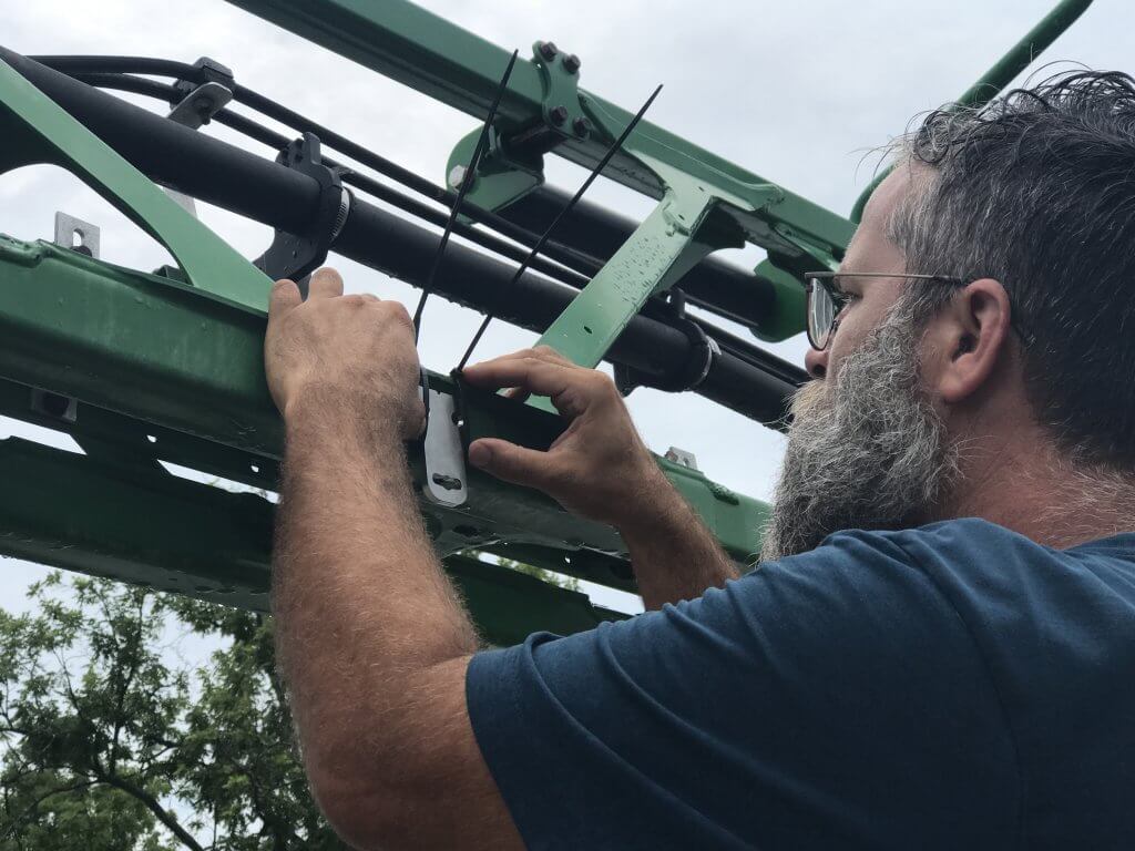
We started by temporarily fixing the mounting plates to the boom using quick ties because we wanted to ensure they did not interfere with boom folding. The drop hose quickly and easily “keys” into the plate allowing it to swing freely and find plumb. The corn was planted on 76 cm (30″) spacing so we aligned the plates with the alleys to permit the drop hoses to move between the planted rows. Each hose is plumbed to the nearest nozzle body via a quarter-turn quick-connect coupler.
Temporarily attaching mounting plates every 30 inches to correspond with corn alleys. The Beluga keys into the mounting plate and is then plumbed into the sprayer via a quarter-turn quick-connect coupler that attaches to the nearest nozzle body.
The drop hose had to clear the ground but still be long enough permit nozzle bodies to span the target region in the canopy. We later learned to cut the excess hose closer to the lowest nozzle body. This eliminated a source of pesticide collection (like a boom end) and prevented them touching the ground and “walking” as occasional contact would cause them them to flex and leap forward.
Target Zone and Nozzle Body Spacing
Before we could permanently install the nozzle bodies on the drop hoses, we had to decide what our target was. This required us to establish a primary coverage zone within the corn. Dr. David Hooker (University of Guelph) experimented with directed sprays (triazoles) and leaf disease control in the 2010’s. Dr. Hooker noted that leaf diseases were controlled above the ear to the flag leaf, and postulated it may be due to xylem mobility (i.e. acropetal movement) of the fungicides used at the time. This concept warrants further investigation with modern fungicides, especially with the need to control tarspot and reduce DON risk in SW Ontario.
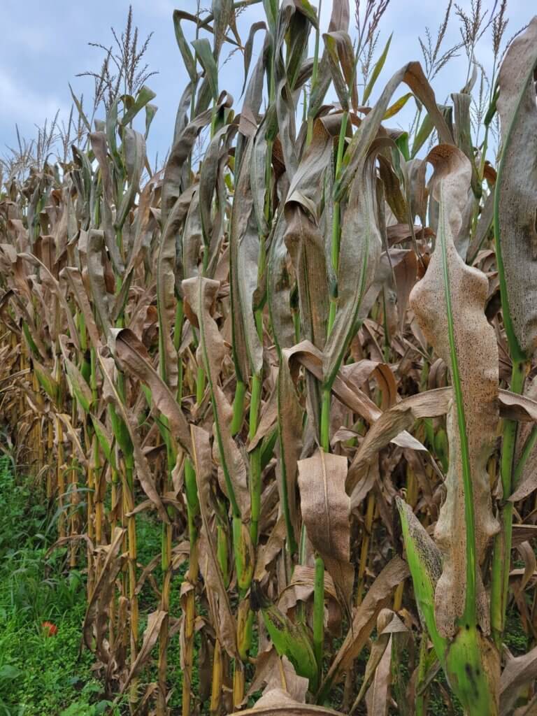
Tarspot in corn – Southwest Ontario, 2023
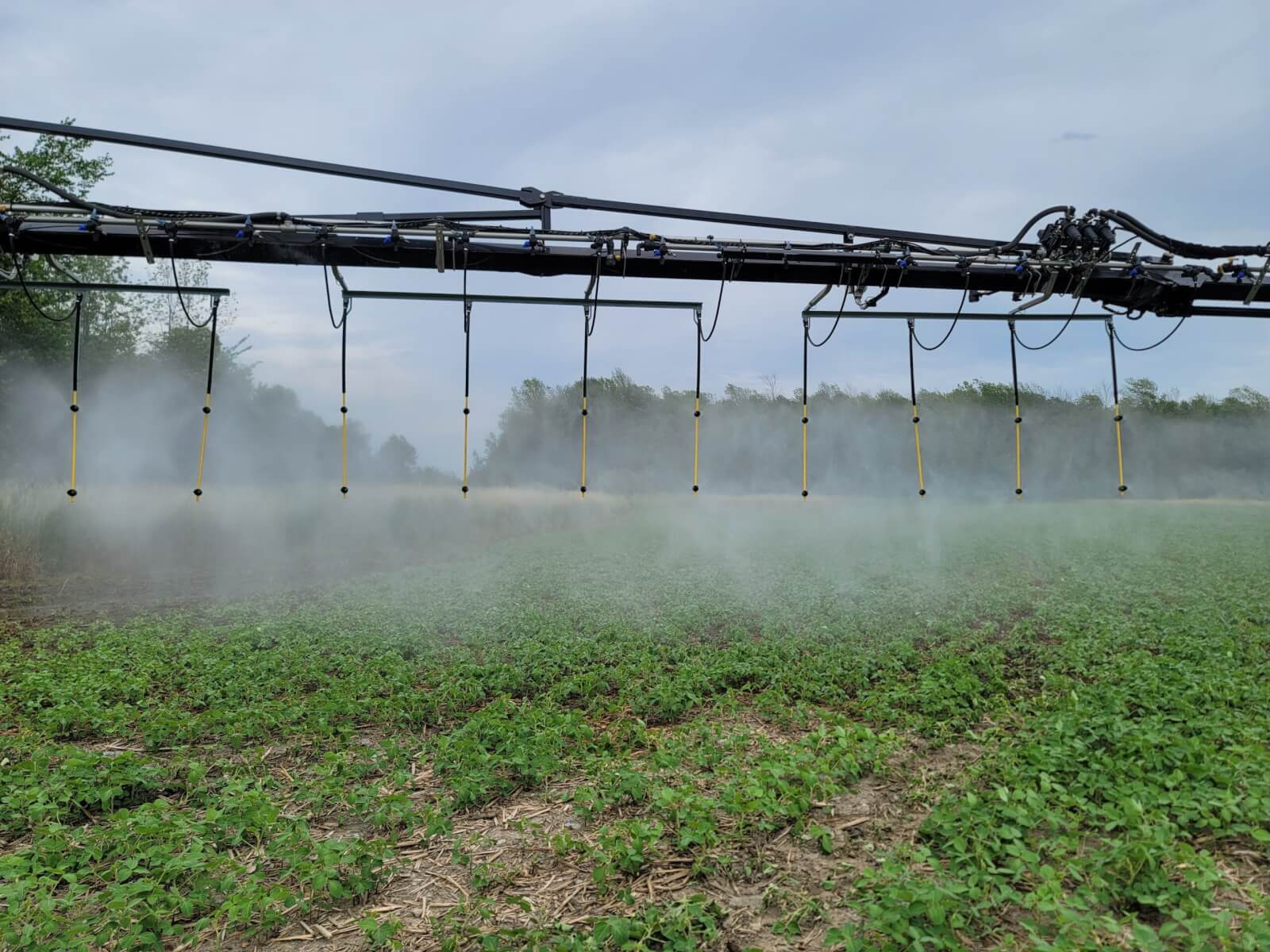
Given that the nozzles would be about 38 cm (15″) from the stalk, we elected to use 110° flat fan nozzles on two nozzle bodies spaced 50 cm (20″) apart to increase the swath. Our objective was to protect against foliar disease, so the bottom nozzle was aimed approximately at the ear (for silk coverage) and the upper nozzle covered the higher foliage without being so high as to spray out of the canopy. Between gravity, the wake of the drop hose, and the initial angle of the spray, all surfaces received some degree of spray coverage no matter their orientation or depth. This was later confirmed using fluorescent dye.
It has been suggested that this target zone may not be ideal for all hybrids, and that an overhead component should be included. However, we felt this was the most efficient distribution of the spray given Dr. Hooker’s observations and the results from the 2019 spray coverage work referenced earlier.
Each drop hose was suspended on 76 cm (30″) spacing to correspond with the centre of each alley. Nozzle bodies were spaced 50 cm (20″) apart to cover the primary target zone within the canopy. The outer two drop hoses only had inward-facing nozzles to contain the treatment. We later cut the excess hose closer to the lowest nozzle body.
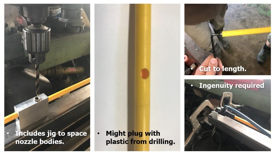
Using the jig provided, we drilled holes for the two nozzle bodies. Then we blew-out the hoses to clear them of any plastic shavings that could plug nozzles. The hoses were cut to length and the end plug was installed with a hex key. Once we found a rhythm, the assembly went quickly and easily. Expect assembly and mounting to take a day.
Customizing the hose length and nozzle spacing. We built our own clamping jig to hold the pipes steady.
Plot Design, Sprayer Set-up and Chemistry
The study took place on 11.3 ha (28 acres) spanning two fields. The corn variety was Pioneer P0720AM, which has a Gibberella Ear Rot rating of 4. Four overhead treatments, four directed treatments and four unsprayed checks were arranged in a random block design for each of two fungicide regimes (n=8 for each treatment per year). Each treatment area was between 1.05 and 1.10 acres..
The sprayer was a self-propelled John Deere R4038 with a rear-mounted 36.5 meter (120′) boom. Treatments were eight corn rows wide, so the boom was nozzled to permit all three treatments in a single pass. Travel speed was between 8.85 – 11.25 km/h (5.5 – 7 mph) and the application volume was 225 L/ha (20 gpa).
Nozzle choice is indicated in the following table. Note that after the first year, we elected to use a smaller droplet size on the Belugas; This gave the advantage of higher deposit density with little or no risk of drift from inside the canopy.
Year
Broadcast (Overhead)
Directed (Beluga)
Unsprayed Check
1
TeeJet AIC11005’s on 15″ centres
4 Airmix 110015’s per drop on 30″ centres
Nozzles blocked
2,3,4
TeeJet AIC11005’s on 15″ centres
4 Spray Max 110015’s per drop on 30″ centres
Nozzles blocked
Treatment nozzles by year
Two tank mix regimes were applied each year, as indicated in the following table. Tank Mix 1 was used each year. Tank mix 2 changed based on pesticide availability and the farmer cooperator’s preference. The insecticide “Delegate” (50 g/ac) was also included in each tank mix. However, there was very little evidence of the target pest (Western Bean Cutworm), so the impact of Delegate will not be discussed. Further, to keeps matters simple, we will not be discussing the relative efficacy of each tank mix in this article. Instead, the results are combined and only the application method and total cost of fungicides will be compared in this study.
Tank Mix (Year)
Product
Rate (/ac )
Tank Mix 1 (all)
Miravis Neo
405 ml
Tank Mix 2 (2021)
Headline AMP + Caramba
303 ml + 405 ml
Tank Mix 2 (2022)
Veltyma + Proline
202 ml + 170 ml
Tank Mix 2 (2023)
Veltyma DLX
202 ml + 405 ml
Tank Mix 2 (2024)
Veltyma DLX
202 ml + 405 ml
Tank mix treatment rates by year.
Qualitative Results
Leaves
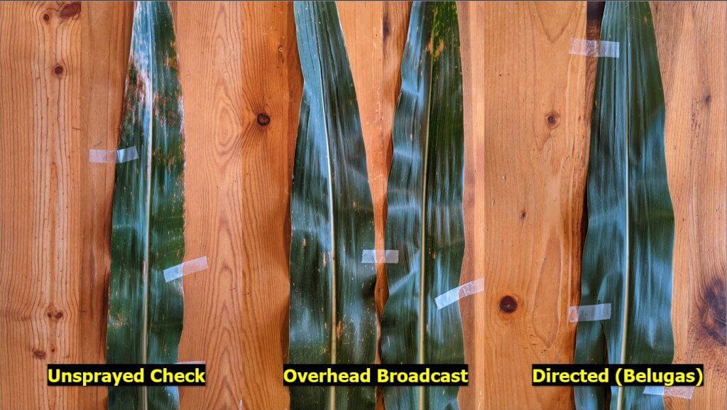
In all four years, a qualitative comparison of randomly-selected ear leaves showed less evidence of disease in the fungicide treatments compared with the unsprayed check. Generally, there was also less evidence of disease in the Directed application treatments versus the Overhead broadcast application treatments.
A typical random sampling of ear leaves were selected from multiple locations in the treatments. Leaves appeared cleaner in the fungicide treatments versus the unsprayed checks. Leaves from the Directed applications seemed cleaner than the Overhead broadcast applications.
Cob Size / Quality
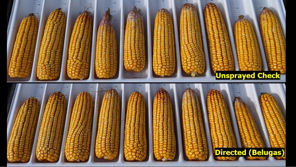
In all four years, preliminary samples showed evidence of disease and tapered-ends in both fungicide treatments and the unsprayed checks, but trends indicated improved size and quality of the cobs from fungicide treatments. It was difficult to discern any difference between Overhead and Directed application at this stage.
Typically, preliminary sampling showed less incidence of disease in the fungicide treatments but no obvious difference between methods of application.
Quantitative Results
Net Revenue
Each treatment yielded corn with different moisture levels, so we chose not to compare bushels per acre harvested. Instead, we calculated net revenue for each year based on the current market values in the Port Rowan area. We normalized the treatment yields by moisture level and calculated their relative drying costs. Then we accounted for the other inputs (see list below) using the following formula:
Net Revenue (CDN) = Seed Yield × Corn Sale Price – Drying Cost – Treatment Cost
Item
2021 ($)
2022 ($)
2023 ($)
2024 ($)
Corn Sale Price (/bu)
6.00
8.00
6.50
6.00
Custom Spray Cost (/ac)
12.00
12.00
15.00
15.00
Drying Cost based on Moisture Levels (/bu)
0.58-0.64
0.60-0.69
0.49-0.56
0.47-0.54
Tank Mix 1 (/ac)
16.66
18.24
18.50
18.86
Tank Mix 2 (/ac)
15.75
28.52
22.09
22.49
Net revenue input costs and prices by year in Port Rowan, Ontario
Averages were calculated for the eight replications for each treatment. These average yields (bu/ac), moistures and ROIs ($/ac) are presented for each treatment, for each year, in the table below. The average values of all four years are also presented in this table. With few exceptions, it always paid to spray, and the directed application produced a higher yield than the conventional overhead treatment.
Year
Treatment
Yield (bu/ac)
Moisture (%)
AverageROI ($/ac)
1
Broadcast vs. Check
-2.26
+0.58
-0.49
1
Directed vs. Check
+3.48
+0.60
+20.93
1
Directed vs. Broadcast
+5.74
+0.01
+21.42
2
Broadcast vs. Check
+9.79
+0.22
+52.48
2
Directed vs. Check
+14.56
-0.04
+89.14
2
Directed vs. Broadcast
+4.77
-0.26
+36.66
3
Broadcast vs. Check
+8.40
-0.20
+23.70
3
Directed vs. Check
+22.7
+0.20
+117.10
3
Directed vs. Broadcast
+14.4
+0.40
+93.40
4
Broadcast vs. Check
+45.7
+1.00
+244.37
4
Directed vs. Check
+43.7
+0.80
+232.09
4
Directed vs. Broadcast
-2.10
-0.20
-12.28
All
Broadcast vs. Check
+13.40
+0.40
+69.07
All
Directed vs. Check
+19.60
+0.40
+107.00
All
Directed vs. Broadcast
+6.20
0.00
+37.93
Final accounting. Bold indicates a desirable outcome, while italics signify an undesirable outcome (n=8 per year).
Return on Investment
Given that costs changed each year, it’s not ideal to average the final costs. However, doing so gives a relative indication of the value of spraying versus spraying with overhead systems versus spraying with directed systems.
Directed (Belugas) vs. Unsprayed check: Profit of $107.00/ac CAD
Directed (Belugas) vs. Broadcast (Overhead): Profit of $37.93/ac CAD
Broadcast (Overhead) vs. Unsprayed check: Profit of $69.07/ac CAD
Perhaps a more realistic review of the ROI is to calculate how many acres were required to pay for the Beluga system each year. In other words, how many acres would a grower have to spray for the profit to offset the cost of purchase? This value was different each year due to changes in costs and relative disease pressure.
In 2021, 48 Belugas on (30″ centres) and 192 110 degree flat fans was $8,400.00 CDN. 2022: $8,600.00. 2023: $8,800.00. 2024: $8,890.00. Perhaps it was demand, or a change in dealers, or perhaps it was tariffs (or both) but in 2025: $13,500.00. Note that the break even point spanned from roughly 40 to 400 acres, but on average was less than 100 acres.
Corn acres required to offset start up costs of the Beluga system from 2021-2024. A broad description of growing conditions and disease pressure in the test fields is noted for context. n=8 each year.
While now a little out of date, the following video filmed by Real Agriculture discusses the return on investment based on 2021 and 2022 data.
Mycotoxin Assays
We submitted samples for lab analysis of mycotoxins for each treatment, annually. However there are many factors that influence ear mould pathogens, and we did not see any clear correlations between the fungicide, application method, or even the unsprayed check with the level of Deoxynivalenol (DON aka vomitoxin) or zearalenone detected.
The Drop Hose Experience
While cost and efficacy are key considerations, we felt it was also important to describe the utility and user-experience. This study focusses on the Port Rowan trials, but over the years several other Ontario farmers have adopted the Beluga system and reported on their experience. We have included their observations:
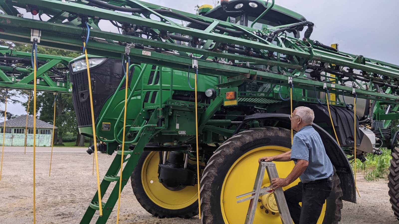
Installing and uninstalling the drops took roughly 90 seconds apiece, including moving the ladder.
Deflection was minimal, even when they were dragged perpendicular to the rows through headlands.
The factory mounting bracket permits the drop to be “keyed in” from either side, however this may have led to drop hoses occasionally detaching in shorter corn stands and on sharp turns. The weak point may be the plastic hose barb, which can be damaged if the drops detach from the mounting plates. Rather than the current slot positions of “9:30 and 2:30”, “11:00 and 1:00” may prevent detachment. One dealer, however, has redesigned the mounting plate and linkage to compensate.
Initially, it was a little unnerving not being able to see the spray but the operator quickly got used to it (see video below).
There was no issue folding the boom or driving between fields with the drops installed. They did note that the lugs on the front tires did contact the drops on tight turns, but adjustments were made.
There were issues with other sprayer types (e.g. New Holland Guardian) when folding the booms. Drops did not hang plumb during transport. One dealer developed new linkages to account for differences in boom design.
The drop hoses rinsed as easily as any nozzle. One dealer developed new hose-end plugs to facilitate rinsing.
There were initial concerns that using 015’s nozzles to maintain the target 20 gpa might cause plugging issues, but none occurred.
The drops were resilient. The operator bent the hoses by lowering the boom and then dragged them along the ground. They returned to plumb and appeared undamaged. One operator elected to use a NutraBoss Y-Drop mount to stiffen the top few inches of the Belugas (image below) but no other user found this necessary.
Once removed, the drops stored compactly and easily on a utility shelf, repacked in their original box or hung on the shed wall.
Beluga drop hoses mounted on a NutraBoss frame
Custom Operators
Some custom operators have also begun to use the Beluga system and have reviewed it positively, but others question the fit. The latter feel this technology makes more sense for a home farm operation where the drops can be cut to a size that aligns the nozzles for a specific combination of boom height and corn variety. The concern is that a custom operator would have to adjust boom height (if not already maxed) or swap drop hoses to configurations that align correctly with the client’s crop. However, four years in, early adopters have collectively sprayed more than 20 different corn varieties with multiple sprayers and have had no issues reaching the target zone.
Additionally, our study has focused on 20 gpa where some custom operators would prefer 15 gpa. Reducing volume necessitates a change in travel speed (may not be practical) or a reduction in operating pressure (may increase average droplet size). It would be inadvisable to drop from 015’s to 01’s (think plugs and misty spray).
Both limitations translate to additional cost (currently about $2.00 CDN per acre) to a client. The value proposition becomes the added cost for an efficacious application versus the potential losses should conventional application methods fail to control devastating diseases such as Tar Spot and Northern Corn Leaf Blight.
Adoption in North America
Beluga drop hoses are distributed by Greenleaf Technologies in Covington, Louisiana and resold through dealers in the USA and in Ontario. It is not possible to determine how many sets have been sold, but if a boom is 100′ to 120′ and drops are placed every 30”, then a set would be 40-48 hoses. We started reporting on their value in corn protection in 2021. The following sales figures are annual sales (i.e. not cumulative) from Greenleaf Tech. This includes the 36″ hoses, which may or may not be used in corn. These figures will be updated annually:
Conclusion
With the exception of 2024, which was essentially parity between Overhead and Directed methods, we saw an annual increase in mean net revenue from corn sprayed using a directed application. The low price point, ease of use, and high rate of return make this an attractive proposition in corn production.
Thanks to Petker Farm Ltd. and other early adopters for participating in the study. Thanks to Corteva and Syngenta for contributing the pesticides used.
In this fourth installment of the Drive-Along Diaries, we’ll shift our focus a little. I’ll continue to share observations about real world spraying practices, but we’ll also dip a toe into the business side of custom application. Every contractor’s situation is different, but perhaps you’ll be able to relate to some of these experiences.
4:30 am
Once again, I found myself driving through Ontario in the wee hours, sipping life-giving coffee and marveling at the total absence of traffic. I was headed to Grande Pointe near Chatham to meet with Paul Delanghe, who’d invited me to tag along with him. I was looking forward, but I was also experiencing a little dread as I imagined subjecting my posterior to another day in the buddy seat. When I arrived at 7:00, I found Paul and his staff in the office. Handshakes were shared all around. Then I dove right in by asking how he got started and how his business worked.
Hello darkness my old friend. I’ve come to sit on you again.
An evolving business model – fertilizer and/or fungicide?
Paul’s family has farmed cash crops, including field tomatoes and sugar beets, for four generations. When he left the aviation industry in 2015, he invested in a high clearance sprayer and a set of Y-drops to apply fertilizer on the family farm. It wasn’t long before he was doing neighbouring farms as well. By 2017 he was saw potential in custom fertilizer work and started Acres Unlimited (AU), which incorporated in 2019.
The original business proposition was straightforward. A split fertilizer application with optimal timing can increase yield while saving fertilizer dollars. For example, perhaps a customer would lay down 150-175 lbs of fertilizer early season, and then call on Paul for another 25-50 lbs using his Y-drops. They might request a single rate, or a variable rate depending on soil type and yield potential (or none if hail or drought wreaked havoc).
This worked well for a few years, so Paul expanded into fungicides. He observed that many corn growers didn’t want to invest in their own high clearance sprayers and preferred to let a contractor worry about minimizing the trample (~4% of the yield). In the case of wheat, many growers were too busy planting to thoroughly clean their sprayers after herbicide applications and were happy to make that the contractor’s problem.
Paul found that fertilizer applications weren’t as lucrative as fungicide applications. High volume fertilizer applications meant spraying 300 ac/day instead of the 5-700 typical of herbicide or fungicide applications. That loss in productivity bit deeper when he had to rely on the client to load UAN because it meant chasing refills and waiting on small-capacity pumps.
Those delays created scheduling conflicts. Typically, as June slips into July, the window for fertilizers closes as the window for fungicides opens. But when there’s a wet spring (like we had this year) it stretches the planting window. Paul would get calls for fertilizer applications in late July, overlapping the fungicide sprays that extended into early August.
So, was offering custom fertilizer still worth it? Fungicides represent the biggest opportunity for profit and are relatively low risk. UAN is hard on equipment and machine prices and depreciation costs have increased significantly (Paul figures $200.00 CAD/engine hour). He calculated that he would have raise his prices to $25/ac for custom fertilizer applications, and that just wasn’t feasible. So, for all these reasons, he decided to leave custom fertilizer applications behind.
Staff roles and coordination
Today, Acres Unlimited consists of Paul, two full time employees (one sprayer operator and one tender truck operator) and one part timer. In addition to working for AU, employees have personal endeavours, such as running their own farms or hauling tomatoes. That means work assignments must be flexible because availability isn’t always a given. Paul sprays from April to November and when he works on his own, he can handle 3 to 500 acres a day. As long as everyone is on board for the peak spraying season in late July / early August it all seems to work.
Staff coordinate their activities through their phones. They drop pins in Google Maps, use a group chat and call regularly to stay in touch. Each employee is trusted to operate semi independently, using their own judgement to establish the safest, most effective, and most efficient means to get the job done. I was left with the impression that the business functioned almost as a cooperative under the Acres Unlimited banner.
7:45 am – The yard
This was great office conversation, and I was so engrossed that I didn’t notice when the staff left for the yard to get ready for the day. We followed behind and Paul showed me their spraying equipment.
The Sprayers
Paul has experience with several asset tracking packages (e.g., AgLeader, Raven), but he likes John Deere’s Op Centre the most. When he started spraying, Deere was the most expensive North American option, so he went with Miller and Hagie. However, the cost of sprayers has increased in recent years and closed the price gap sufficiently for him to justify buying a 412R in 2023. AU also runs a 2022 Miller Nitro 7310, and that’s used by their second operator.
According to Paul, Deere really isn’t interested in producing a high clearance machine for corn (he was encouraged to go buy a Hagie) so he had to add tall tires and a lift kit to climb from the 1.53 m (60”) stock clearance under the frame to 1.82 m (72”). He also protected the hydraulics behind the tires by covering them with canvas bags. Other growers use 5 gallon pails or even car mats to accomplish the same thing.
Tendering equipment
AU recently upgraded to a Phiber DASH 4.4 on their 15,900 L (4,200 gallon) tender truck. It caused a little sticker shock but paid for itself very quickly. The sprayer was no longer idling while the operator filled the bowls, saving on engine hours. Plus, the less than eight-minute fill time added to their overall productivity.
The tender truck itself was designed for the operator to forklift totes onto an overhead platform and gravity feed chemistry into the inductor bowls. Paul likes the bulk format over the jugs and uses it whenever it’s feasible. However, he installed transfer pumps because they’re faster than gravity feed and do a better job emptying the totes completely. Paul prefers to trust the embossed sight gauge on the side of the bowls over a flow meter; Variability in product viscosity makes the flow meter inaccurate, and that adds up over several loads. In fact, when using totes, they’ve seen discrepancies as high as 50 L (13 gallons) at the end of a day.
There was also a humble 1994 cube truck to service the other sprayers with diesel and chemistry, and a 27,250 L (7,200 gallon) water truck. AU gets their water from municipal stations, and one was conveniently located across the street from the yard. It’s a fast fill, and while there’s rarely a line up, they still make sure to fill each night to ensure an efficient start the next morning.
Float trailer
Chatham-Kent and Essex are big counties. When Paul ran the numbers on engine hour depreciation, the operator’s time, fuel, maintenance, and tire wear, floating the sprayer between jobs made sense. So, he uses a 12,100 L (3,200 gallon) float trailer to transport his Deere 412R.
He chose the two-bowl Phiber DASH 2.4 because they use a lot of jug formats with this sprayer. The left bowl (J) is a push-to-rinse system and on the right (R), a knife. This is handy for co-packs. For example, Veltyma DLX is a co-pack with one larger and one smaller jug. The smaller jug gets upended on the rinser and the larger jug gets spiked on the knife. Spiking is faster, but there’s always a chance of stabbing yourself, so better to spike the larger jugs.
8:05 – Heading out
While I waited, Paul circle-checked the float trailer. Then he flipped open the tractor trailer hood and climbed inside to get it to start! He explained that he had to manually operate the fuel pump because the electrical was cranking too slowly. This truck had almost 1,000,000 km on it and fixing the pump was going to be ~$7,000.00, so this little work-around was fine with Paul. Plus, it’s great anti-theft security.
We drove on narrow county roads which required us to lean on the gravel curbs. Paul noted that it typically kicks up a lot of dust and aggravates the people driving behind him. It can spur them to passing unsafely. But since we’d had so much regular rain this season, there was no dust and people seemed more patient.
This isn’t actually Paul, but only a few weeks after spending the day with him I ended up driving behind a sprayer. The photo op was too good to miss. and yes, I passed him.
8:18 am – Loading
Now at our destination, Paul found a safe and accessible place to park and began untethering the sprayer. That consisted of removing the four chains with turnbuckles that secured the sprayer to the trailer. He always does this first, so he doesn’t forget before backing it off… ask him how he knows. This took about two minutes to complete. Then he hit a switch under the sprayer to send up the airbags and grabbed some gloves to start filling the inductor bowls.
As Paul was pouring chemistry into the inductor bowls his phone started ringing. He said he never answers when he’s focused on loading. It takes time and attention to ensure it’s done right, and he didn’t want any distractions. Paying a little extra time and attention now means avoiding costly issues later.
This was a 54 ac job, but Paul was adding enough for 60 acres because he didn’t want to run short. A little leftover fungicide on the next job (soybeans) would be a nice bonus for the client. Each jug was emptied, rinsed immediately, had the cap replaced and was dropped back in its cardboard box. The water truck operator would grab them later when he came with our refill. Removing caps and labels for recycling is a rainy-day job.
Prepping jugs and cardboard for recycling is rainy day work.
The loading process
Perhaps I should have explained sooner, but here’s a short and generic description of the chemical loading system. Product gets added to a conical inductor bowl. This can be via jug (poured or knifed), or from bulk containers via gravity or transfer pump, or dry products get blended with a recirculating agitator. One of several bowls might be filled, each with their own product, or one bowl can be filled and emptied serially. Then the operator starts the carrier pump and begins pushing carrier (usually water) into the sprayer tank. Once enough is loaded, a valve at the bottom of the bowl is opened and the Venturi effect creates suction to draw the chemistry into the carrier stream. Then a second valve is opened to activate a rinse head in the bowl, or this is done manually using a hand-held hose. This process can then be repeated to separate products and control mixing order. Finally, it’s followed up by more carrier to rinse the lines and finish filling.
Alternately, the suction pump on the sprayer itself can draw in carrier and the induction bowl on the side of the sprayer can be used to add chemistry. In a similar fashion, onboard water is used to rinse the jug and the bowl.
Paul used a hybrid of these two methods by engaging the pump on the tender system and the pump on the sprayer simultaneously to speed up the process. There are some caveats to doing this. The concern is that some formulations may cause damage to the sprayer pump, but Paul feels there’s so much carrier water following behind the chemistry that it flushes the pump and the entire line. Here’s how he did it.
Paul backed the sprayer off the trailer and hooked up to the front-fill. He started the pump on the DASH to add about 750 L (200 gallons) of water to the 4,540 L (1,200 gallon) sprayer tank. This was not the ideal “half full”, but unless he’s anticipating a mixing issue, that’s all he uses. In situations when he’s pushing multiple products into the sprayer, he’s found that the tank can fill before he’s done. Ironically, that’s when it’s so important to start with more water, but I’ll get off my high horse now.
He had already poured or knifed products into the bowls, so he opened the valve under the first, drawing the contents into the water stream before rinsing the bowl down. Then he did the second. Then he walked over to the sprayer and started the sprayer pump to add a “pull” to the “push” and speed up the fill before returning to the DASH to wait.
Paul said he’d installed an Accu-Volume on his Miller sprayer (and loves it) but saw no need for it on the Deere. He said the float in the tank quickly and accurately responds to the level in the tank. At that point the sprayer registered as “full”, the sprayer pump automatically shut off and the valve closed. You could hear it happen. But the DASH was still pushing and would quickly stretch and damage the hose, and even cause leaks.
That sound was Paul’s cue to quickly shut off the DASH pump. Then he closed the Banjo quarter turn valves on either side of the connection and disconnected the feed. He said he never pushes UAN through this system. Ag retailers don’t use flow meters with UAN because they can be inaccurate – instead they use weigh scales. However, it was too hard to navigate an oversized tender truck onto a scale, so UAN got loaded directly.
At 8:32 we were filled and ready to go. That was 14 minutes from the time Paul started untethering to when he started backing the sprayer off the tender truck. And it would have been a lot faster if he hadn’t taken time to explain it to me.
8:35 am – Job 1
At the edge of the first corn field, Paul unfolded the boom and set up the monitor. We would be applying 20 gpa at 60 psi and travelling about 12 mph. When spraying corn, Paul tends to travel between 10 and 14 mph. He double checked that the pneumatics he’d switched on earlier had lifted the sprayer high enough to clear the corn.
One of the chemical companies had given him a set of Low-Drift Air 11005 flat fans (PSLDAQ1005) to try, and this was his first time using them. We immediately saw that they were not all pointing in the same direction (or even alternating). They were just on willy-nilly. We figured it wouldn’t matter since we were only just clearing the tassels, but it tweaked both of our latent OCD personalities and we decided to fix them next chance we got.
Nozzles tilting at windmills – just not all in the same direction.
We finished at 8:59 am and found we’d covered 51 of the estimated 55 acres, due in part to a few missed strips and rounded-off corners. Why did we miss them? Read on.
Fungicides versus herbicides and fertilizers
I’d tagged along during fertilizer and herbicide applications, so I began to notice that overhead fungicides in corn seemed to follow different rules. Here are some observations I made throughout the day:
It’s not ideal to have to stretch a tank of herbicide, but you can if it’s not too dilute. And you can always go top up if you really must. However, for fungicides, you absolutely do not want to run short because that means increased trample. You can stretch the tank a little, but if it means running over corn, then leaving a few “test strips” and unsprayed corners is the profitable choice. Quote from Paul: “The most important part of fungicide in corn? Don’t run over the corn.”
Paul felt sectional control was more than enough resolution for fungicide applications in small/medium sized fields. The uniformity and product-savings associated with nozzle-level resolution (e.g. PWM with turn compensation) pays with herbicides and expensive fertilizer, but not fungicide.
A low and steady boom is ideal, but not critical for corn fungicides. Increased drift potential and a loss of coverage uniformity are still bad practice, but rather than slow down and drop the boom, we leaned into maintaining our speed and raised the boom ends until they were clear of the tassels. Even then, the centre rack was still deep in the canopy. C’est la vie.
9:00 am – Job 2
Job two was the for the same customer, so all we had to do was cross the street to a 60 acre soybean field waiting for an application of Delaro Complete. This time we were full in seven minutes (because I didn’t ask silly questions) and we were starting to run short of water. We called for more.
I haven’t mentioned it, but the Deere was equipped with Precision Planting’s ReClaim recirculating booms. He was actually one of the prototype testers, having installed it on his old Patriot a few years back and his Miller as well. I’ll discuss the system in more detail later on. So, at 9:10 am we started recirculating the boom to dilute the residual Veltyma DMX and prime the Delaro Complete. Veltyma DMX has some “greening effect” on soybean, so while a full dose wouldn’t hurt anything, it would leave a conspicuous green triangle at the edge of the field that no one wants to see.
We drove the perimeter manually. The ruts left from such a wet year kept tugging the sprayer, so Paul steered with a light touch, correcting when the wheels pulled. Once we got to the interior, we were applying 20 gpa at 13 mph. Paul relied more on autosteer (although he still fought the ruts a bit) and took the opportunity to text customers and get in touch with staff. Just as when he’s focused while loading, never taking a call, he doesn’t take them when spraying field boundaries. At 9:39 we were empty and done.
Acquiring and scheduling customers
I asked how AU found and scheduled customers. Paul said that roughly 40% of their business came from contracts with ag retailers and the remainder was direct. AU works with a few ag retailers, and they don’t all operate the same way. Here’s how it was explained to me.
Ag retailer 1 acquires a customer and sells them any number of agronomic services, including crop inputs. Then they use their own sprayer, or subcontract someone like AU to spray those crop inputs. AU has the option to decline a job (perhaps it’s too small, too distant, or generally undesirable), but they can’t do that too often. If they accept, they pick up the chemistry and apply it within 24 hours to avoid long-term storage.
Ag retailer 2 has a different arrangement. In this case Paul refers to a project management app called “Monday.com” which allows him to review and select open jobs. Once again, they pick up the chemistry and apply it within 24 hours.
AU also takes on customers directly. Weather events and breakdowns are problems for farmers but represent opportunities for contractors. AU is often hired by large farming operations (e.g. >1,000 ac) when they can’t keep up, and this is far better than chasing 10-15 ac fields.
Juggling all these customers can be challenging. In the winter, the core, repeat customers are penciled into the schedule. However, in the chaos of fungicide season, the ag retail customers get priority because of contractual obligations. And, of course, AU is always open to opportunities and slots in new jobs as best they can. They take advantage of social media while operating because Paul believes it’s important to stay involved in the community, but also because it’s a means of free advertising. People see when they’re in the area and it’s resulted in lots of jobs.
Duck hunting
I debated including this in an already epic article, but it was too interesting to leave on the cutting room floor. Paul also described a long-standing niche job working as a land manager for a few private “duck-farm” operations. Nearby Mitchel’s Bay is some of the best duck hunting in the world because of strategically placed duck-farms next to marshes or lakes. They grow corn to attract the ducks, then mow parts down to make pathways for boats, and then flood the fields using dikes and pumps.
These clubs aren’t necessarily big revenue generators. They’re perks for businesses to offer employees, or locales for casual business meetings, or maybe just status symbols for the wealthy elite. Given that they spend a lot of the year flooded, the ground is tough to spray because it’s always soft. Sprayers can’t go in full, and that tends towards premium fees for crop management.
Paul sprays for a few of these operations because he finds the whole practice fascinating. And, as a duck hunter himself, he’s permitted access to places most never see. There’s no such thing as free corn, Daffy.
9:43 am – Water fill
The water truck arrived and six minutes later we were topped up. Then it left to go support the Miller about 30 minutes away, promising to come back to us right after. Paul appreciated not having to go back to the yard for water – how can you ever be satisfied with coach after you’ve flown first class? We headed off to the next job.
Paul made this look easy.
9:51 am – Job 3
This 50 acre soybean field abutted a tomato field, and after seeing this sort of thing all season I wondered aloud if buffer zones were just a white lie that we tell ourselves. Paul chuckled and said there’s generally no stress when spraying fungicide this close to a sensitive crop, but herbicide would be tense. He changed fields on the monitor, verified that he was applying the right amount and started spraying. He noted there was a soft area in the field where the owner replanted soybeans. We avoided it.
This was one of the direct customers and not an ag retail client. The customer was a tradesman that left the crop protection choices to Paul. Custom operators can have a lot of influence on their client’s product choices because they spray so many acres with so many chemistries. In order to better guide his clients, Paul makes an effort to get involved in product testing and performance trials. But, as a sprayer operator, he’s not only interested in efficacy and price, but also ease-of-use.
Running a product comparison trial
For example, powdered manganese plugs a sprayer horribly while liquid formulations are far more forgiving. Another example, perhaps one product is 1 L/ac while another is 2 L/ac. Handling less is always easier. Or perhaps all this is trumped when a customer is swayed by loyalty points, which are issued by some registrants to reward a customer for using their suite of products.
We were done at 10:11 and found we’d covered 47.5 of the 50 acres because we skipped that wet, replanted area. That left about five acres worth of spray mix in the tank that we’d have to consider on the next job.
Recirculating booms
Paul secured the sprayer to the trailer, and we hit the road. While we drove, he talked about why he felt a recirculation system was necessary. Beyond the savings in chemistry and water, he said it was tricky charging the boom on some of the farms in the county. Severed lots meant more homes and private gardens, and that limits where it’s safe to prime.
Precision Planting released their aftermarket ReClaim recirculating boom a few years ago. We’ve written about it. Basically, it relies on dropping the pressure below the ~10 psi required to open the check valves in the nozzle bodies. So, no shut-off valves required. However, some Deere pumps won’t operate under 20 psi, which requires a work-around. Despite having that fix in place, we still saw nozzles dribbling while we were recirculating. Obviously not ideal, but Paul said it cost about a seventh of what the factory option would have cost, so he could live with it.
But there are other points to consider. For example, the sprayer doesn’t know the feature is there. So, when recirculation is engaged the sprayer “thinks” it’s spraying, and as liquid passes the flowmeter, the display shows the volume dropping… but it isn’t. As a result, the operator must know how much liquid circulated and manually adjust the volume prior to spraying.
And this system isn’t plumbed to flush the lines from the clean water tank. And it increases the length of hose that needs to be rinsed. And while you can recirculate glyphosate and UAN, many operators won’t do it with sticky products like atrazine or dicamba, preferring to just prime normally and keep them out of the recirculation lines.
While Paul and I were discussing all of this, and you can’t make this stuff up, the second operator called to say they broke an elbow on their recirculation line. To their credit, Precision was out there like a shot and had it mended in an hour (amazing service). But the delay meant we had to redistribute some of the remaining jobs. It was decided that Paul would take on some extra work and then both operators would meet up at the end of the day and split the last job.
10:50 am – Job 4
We parked, dismounted from the trailer, loaded and taxied to the headland. Paul said it was another 50 acres of corn, but I saw something was different. He treaded out the tires to a 138″ spacing to align with what I was told was a 23” corn spacing. Until now, we were on a typical 30” planting architecture. I soon learned that I didn’t like 23” corn. Tracking between such tight rows without trampling everything was a nightmare.
Here are two videos. We’re driving 30″ corn in the first and 23″ in the second.
I asked if Paul had tried row feelers, but he said they didn’t work on such tight spacing. In any case they got in the way when he used his float trailer. So, I watched as Paul studied the row ahead and referred to the feed from the cameras, micro-adjusting the steering for the entire 47.8 acre field as he fought to stay between the rows. It felt like forever, but we were done at 11:24 and back on the road for tendering a few minutes later.
11:38 am – Job 5
As we drove alongside this 45 ac field to get to the entry, we saw rows of sweet corn planted on the perimeter (surprise). Paul said there was a variety trial planted in the centre of the field somewhere as well and that we weren’t supposed to spray it. And it was another 23” row spacing.
Once again, we found it hard to stay on course. Just for added fun we got pulled by the planter draft and the occasional guess row. We finished at 12:10 pm and planned to meet the water truck. As we left, Paul reset the treads to 120” from 138”. Never good to forget that bit – again, ask Paul how he knows.
1:07 pm – Job 6
After a short and uneventful drive to the next client, we parked, loaded, and unfolded at the headland of a 45 ac cornfield. As we sprayed, Paul was on the lookout for a bridge that would give us access to another, smaller field. It turned out to be a substantial land bridge, which disappointed Paul because he was hoping to take me over a rickety little wooden bridge. The buddy seat was rough enough without testing its absorptive qualities as well, so I was good with it.
There were plenty of obstacles in this field. Paul was well acquainted with “the tree”. They’d had dealings in the past. I asked about wind turbines, which were all over the county, and I was surprised that he liked them. All turbines in the area have associated hard-packed lanes leading through the field. Paul took advantage by parking on them and filling there if needed. Plus, he watched them to monitor wind speed and inversion situations.
Still on the subject of obstacles, we found a field of peppers hidden in the corn. We left the test strip there. As we made these on the fly decisions, Paul wondered how an autonomous sprayer would handle all these little surprises. A good question.
I was finding the rows a little hypnotic and said so. Paul said corn was hard to spray day after day. In windy conditions, the tassels sway and it can make an operator dizzy. Some operators slow down to 10 mph or use row feelers to stay on track. We finished at 1:37 and when we got back to the trailer, two new jobs came in over the phone. Paul decided that his other operator could absorb those. We got ready for what might be our last job – rain was forecast
1:58 pm – Job 7
Full again, this 74 acre corn field would also get a test strip. Paul reiterated that it’s better to trample a field once, and not go in and out to get more spray mix. So, we filled for 70 acres spraying at 17 gal/ac and 9.6 mph to empty a single tankful as accurately as we could.
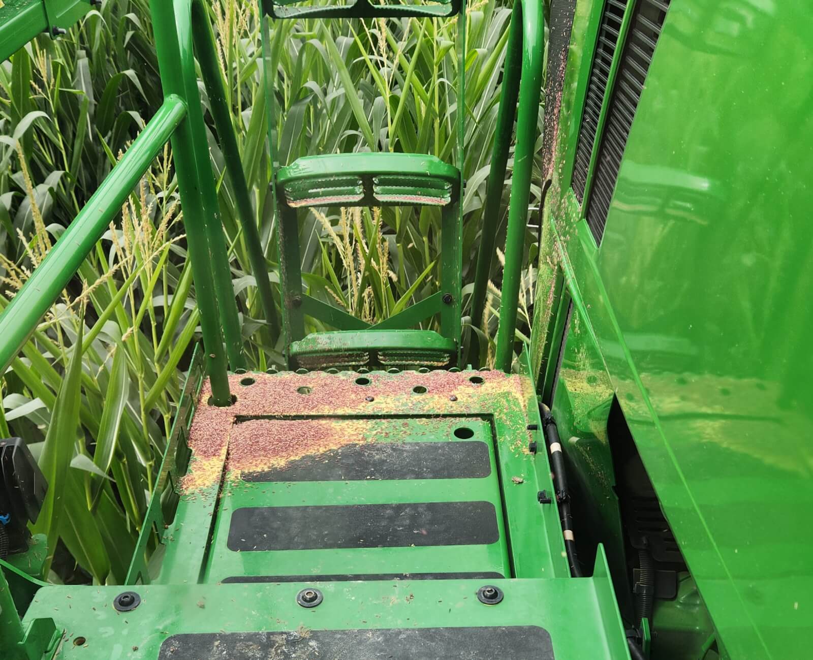
I watched as the pollen and anthers broke in waves over the hood and onto the steps. The radiator fan periodically reversed to blow it all out, but not as frequently as we needed. Paul occasionally did it manually. The sound of corn scraping and hitting the sprayer was loud. Paul said corn can beat the paint off a sprayer and damage the side induction bowl – wow. Carbon filtered cab or not, my pollen allergy was driving me crazy, and I was glad this was our last job. We were done at 2:37 and back on trailer five minutes later.
3:30 pm – Back at the yard
As we pulled into the yard it looked like rain was indeed coming. We weren’t worried about the fungicides we’d applied because they were rainfast in an hour. But it did put a premature end to the spray day. We’d covered more than 365 acres in the Deere, which was a light fungicide day for Paul. Combined with what the Miller did, AU covered 735 acres.
As I was packing to leave Paul asked if I was interested in seeing his new battery-powered backpack sprayer. I was, but I didn’t realize he’d put me to work spot spraying weeds. So, I suppose we actually covered 736 acres that day: 735 in sprayers, and one manual. Worth it.
This work was performed with Mark Ledebuhr (Application Insight LLC.), Adrian Rivard (Drone Spray Canada) and Adam Pfeffer (Bayer Crop Science – funding partner). Amy Shi is gratefully acknowledged for her assistance with statistical analysis.
Introduction
In June 2017, Transport Canada cleared the general use of drones. In 2018, Health Canada clarified that the use of Remote Piloted Aircraft Systems (RPAS) for pesticide application is not permitted under the Pest Control Products Act without sufficient data to characterize any associated risk. Currently, there are no liquid pest control products registered for application by drone in Canada.
Stakeholders want to use drones to apply pest control products in Canada. To that end, several research trials have been approved by Health Canada. However, multi-rotor drones represent a unique application technology more akin to air-assisted ground sprayers than manned aircraft. As such, conventional models for drift, exposure and efficacy may not apply. Fundamental questions surrounding the utility of drones must be addressed before efficacy and residue can be considered in any relevant context.
Research and user experience has identified, and is beginning to understand the relative influence of, external factors such as crop morphology, planting architecture, topography, and environmental conditions. Considered with the product mode of action, these factors inform operational settings such as altitude, travel speed, nozzle choice, and application volume to optimize applications. This collective “Use Case” depends on drone design, which is highly variable and rapidly evolving.
Having performed preliminary work characterizing effective swath width, and recognizing its popularity in North America, we used DJI’s Agras T10 in this study. Our objective was to evaluate fungicide efficacy on Northern Corn Leaf Blight, Tar Spot, Grey Spot and Common Rust in field corn, as applied using the T10. Drift and coverage would be characterized to provide context for the efficacy analysis, but also to develop data to inform best practices and possibly regulatory decisions surrounding risk. Aspects of the study would be repeated using conventional ground sprayer technologies to form a basis for comparison.
Objectives
Quantify spray coverage in field corn at three canopy depths, on adaxial and abaxial surfaces, as recovered tracer dye (indexed to % of applied rate ac-1), area covered (%) and deposit density (deposits cm-2).
Quantify drift as recovered tracer dye (indexed to % applied rate ac-1) collected using the horizontal flux method up to eight meters high on the immediate downwind edge of the application.
Evaluate the fungicide efficacy, applied using the T10, at 2 and 5 gpa as compared to a conventional overhead broadcast treatment at 16.7 gpa.
Material and Methods
Design
Trials were conducted between July and August of 2022 in three Ontario corn fields. The locations, the application methods and data collected are detailed in Table 1.
Field
Location
Corn Variety
Application Method
Rate (gpa)
Data Collected
1
Jaffa (42°45’56.6″N 81°02’06.5″W)
DKC45-65RIB
Agras T10
2 and 5
Drift, Coverage, Efficacy
Overhead Broadcast
16.7
Coverage, Efficacy
2
Fingal (42°42’17.9″N 81°15’15.3″W)
DKC49-09RIB
Agras T10
2 and 5
Drift, Coverage, Efficacy
Overhead Broadcast
16.7
Efficacy
3
Port Rowan (42°35’53.6″N 80°30’43.2″W)
P0720AM
Directed (Drop hoses)
20
Coverage
Table 1 – Trial sites by application method and data collected
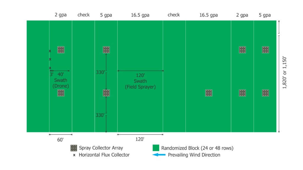
Treatments were arranged in a randomized complete block design (Figure 1). Corn was planted on 30″ centres, with about 6” in-row spacing between stalks. We targeted spray for the R1 stage of development (approx. 8’ high). Fields 1 and 2 each hosted two replicated treatments of 2 gpa, 5 gpa, and 16.7 gpa, as well as two unsprayed checks. In field 1, blocks were 60’ (24 rows) wide by 1,150’ long for the T10, and 120’ (48 rows wide) by 1,150’ long for the broadcast field sprayers. A single, 120’ swath was applied using the field sprayers, and four 10’ (4 row) swaths were required to spray the centre 40’ (16 rows) of corn using the T10. This was based on a 10’ effective swath width determined in previous research. Field 2 had a similar layout but was 1,820’ long.
Figure 1- Sample experimental layout for Field 2. In this example, horizontal flux collectors are positioned 3’ downwind to intercept any off-target drift from the edge of the adjacent 2 gpa treated area.
Coverage Analysis
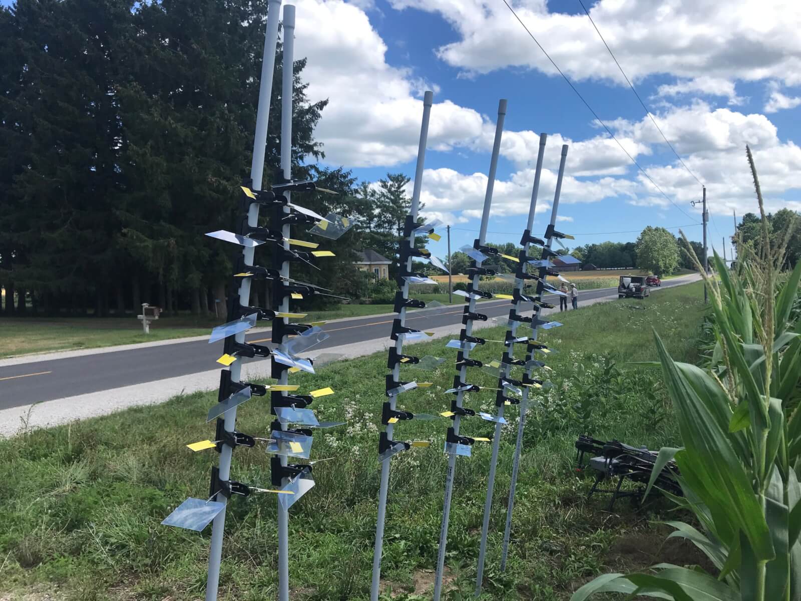
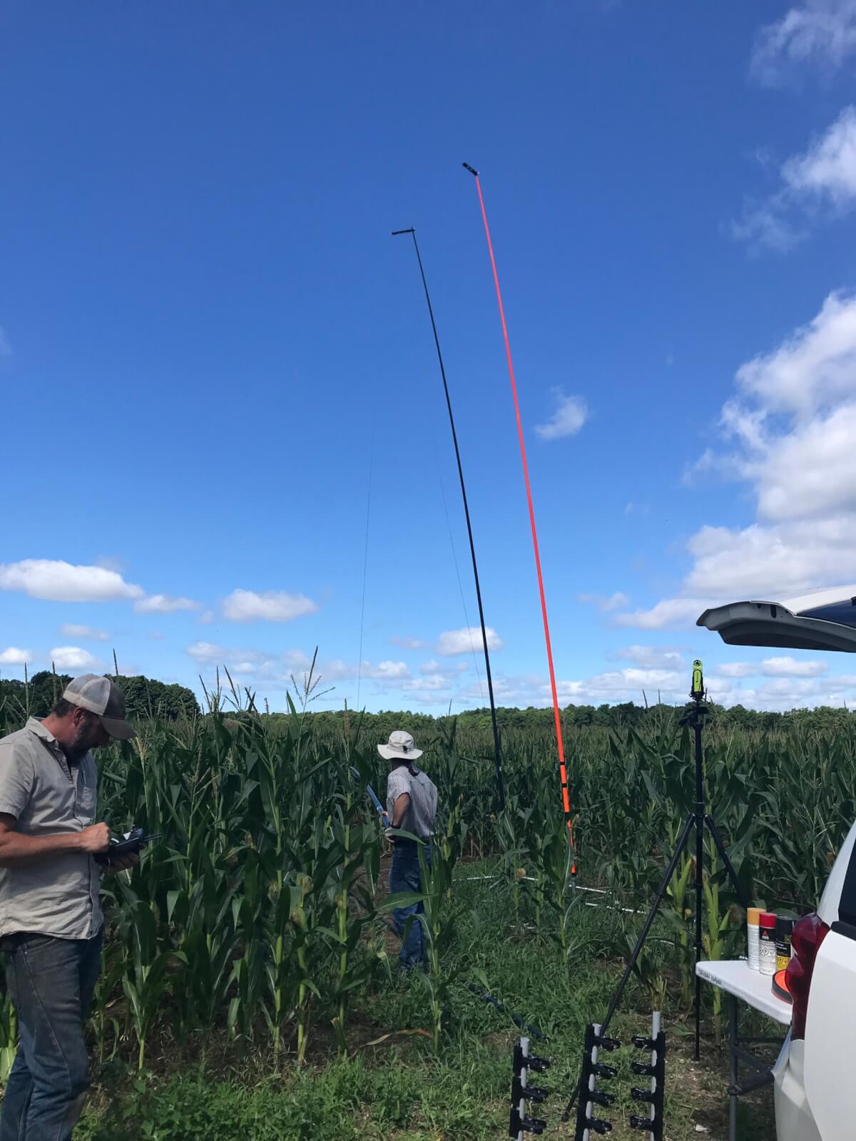
To account for variability, each treatment block was subdivided into two regions, each containing an array of nine spray collectors. Each spray collector (Figure 2) consisted of a vertical, 8’ pole in-row between corn plants. Samplers were attached at three depths to span the silking region: Top: 1.5’-2’ below the tassel. Bottom: 1.5’-2’ from the ground. Middle: halfway between them. Samplers were parallel with the ground to ensure the highest degree of spray interception. On one side, two 1”x3” water sensitive papers (WSP; Innoquest Inc.) were clipped back-to-back with a sensitive side positioned up (adaxial) and facing down (abaxial). The other clip held two 4” square sheets of Mylar in the same orientation. Sampler type was alternated vertically (e.g. Mylar – WSP – Mylar or WSP – Mylar – WSP).
Figure 2- Spray collectors temporarily loaded with WSP and Mylar samplers. These were held above the tassels as they were carried to the collection sites in each block. Three clips were positioned per pole, alternating Mylar and WSP samplers on each side, on two arrays of nine poles, as previously described.
This study used 864 WSP and 864 Mylar samplers for the RPAS treatments, and 162 WSP for the overhead broadcast and directed applications. Following the application, samplers were retrieved as soon as they were dry enough to handle (about 30 minutes) and individually placed into pre-labeled sealable plastic bags, each uniquely coded to the exact position and orientation of the collector.
Operational Use Cases
5 gpa: DJI Agras T10 was operated at 3.3 m/s, 2 m above tassels. TeeJet 11002 AIXR nozzles equipped with 50 mesh filters were operated at 70 psi.
2 gpa: DJI Agras T10 was operated at 7.0 m/s, 2 m above tassels. TeeJet 11002 AIXR nozzles equipped with 50 mesh filters were operated at 45 psi.
16.7 gpa: Overhead broadcast condition. Field 1 ran a John Deere 4038R operated at approx. 10 mph with TeeJet XR11006 nozzles on 20” spacing. Pulse width modulation (ExactApply) was engaged. Field 2 ran a New Holland 345 front-mounted boom sprayer with TeeJet XR11006 nozzles on 20” spacing.
20 gpa: Directed condition. John Deere R4038 operated at approx. 4.5 mph with Beluga drop hoses suspended on 30” centres to correspond with alley spacing. Two nozzle bodies were positioned 15″ apart equipped with Greenleaf Spray Max 110015 nozzles to span the silking area.
Drift Analysis
Three free-standing 26’ (8 m) horizontal flux collectors were positioned in the corn field approximately 3’, or 1.5 rows from the downwind edge of the spray plot downwind of the area treated by drone (Figure 3). The sampling poles were positioned about 30’ apart parallel to the treatment block. Sterilized, 1.8 mm braided polyethylene collector line was run up the poles on pulleys just prior to application. Following applications, the line was collected in 1 m lengths into sealed bags.
The assumption was that by placing the horizontal flux samplers as close to the “zero” downwind edge position as possible, nearly the entire off-swath movement of drift would be captured. A compromise of placing the samplers in the middle of the first row past the downwind swath edge was made due to the scale of the sample and the relative low swath precision of the drone. Placing the samplers closer to the zero downwind line was deemed to be too high a risk of inadvertently sampling in-swath.
Figure 3- Moving horizontal flux poles into the field prior to positioning them for trials. String collectors were run up the poles just before spray application and retrieved immediately afterwards.
Spray Solution (Formulated Product plus Tracer)
Fungicide was applied at field rates (8 oz/ac or 586 mL/ha). The field sprayer applied this at 16.7 gpa. The drone applied it at 2 or 5 gpa but also included tracer solution at 0.2% (20 ml/10L solution) vol./vol. of a 20% mass/mass solution of PTSA in dH2O. PTSA residue data assumes 100% recovery and 0% degradation of the tracer. Tests of PTSA with fungicide prior to the study showed no physical antagonism and >98% tracer recovery. Prior testing of PTSA showed an acceptable 1-2% solar degradation in the timeframe required to collect samplers. Tank samples were drawn from the drone at the beginning and end of each trial and used to confirm tank concentration and to establish fluorescence curves.
Weather Conditions
Weather data was collected using a Kestrel 3550AG weather meter (Kestrel Instruments) in a vane mount positioned 1 m above the tassel (approximately 1 m below drone altitude). Data was logged every 5 seconds. Issues with data loss required us to supplement local data with Field Level Weather Summary data (Table 2).
Date (2022)
Field
Vol. (gpa)
Avg. Temp. (°C)
Avg. Windspeed (km/h)
Start Time
Duration (min.)
Jul 25
1
5*
22.3
6.2
13:00
35
Jul 25
1
5
21.4
7.5
18:45
35
Jul 26
1
16.7
18.8
5.4
10:00
45
Jul 26
1
2
23.9
7.7
15:30
25
Jul 29
2
5**
n/a
16.4
11:00
35
Jul 29
2
2***
23.6
21.0
14:00
25
Aug 12
3
20****
25.4
6.3
13:30
15
Table 2- Date, location, and weather conditions for each treatment *Trial pass over spray collectors only – no horizontal flux collectors employed. **All bottom-level water sensitive paper samplers spoiled by high humidity. Wind changeable and horizontal flux poles moved 2x before application to orient downwind. ***Noted flocculation in tank samples likely from rainfastness adjuvant. Did not affect analysis. ****Coverage data from a single array of nine spray collectors with water sensitive paper samplers.
Results
Statistics
The % applied rate ac-1, % area covered, and deposits cm-2 were subjected to analysis of variance using SAS® OnDemand for Academics PROC GLM. When a significant treatment effect was found, means were compared using Tukey’s honest significant difference test (HSD) at p=0.05.
Data Collation
Each spray collector was a vertical structure that supported Mylar samplers at three depths. Each depth held two samplers oriented abaxially or adaxially, in parallel with the ground. When discussing the amount of PTSA recovered by sampler depth or by sampler orientation, the % applied rate ac-1 of each of the nine related samplers were averaged within each array (n=2 arrays per block times two replicates equal n=4 per treatment).
When considered from above, the six Mylar samplers are vertical cross-sections of the same area of ground. Therefore, the % applied rate ac-1from each sampler was added to represent the total mass of tracer intercepted per collector. When these nine sub-samples are averaged, we arrive at the average % applied rate ac-1 per array.
Similarly, the % applied rate ac-1 from each 1 m length of string on a horizontal flux collector could be averaged across collectors by relative position to explore drift by height (n=3 poles per block times two replicates equal n=6 per treatment). Alternately, the total PTSA recovered per pole could be calculated (n=3 poles per block times two replicates equal n=6 per treatment). This interpretation allowed us to perform a mass balance accounting of residue in-canopy and as drift compared to the known applied rate ac-1.
It was not possible to collate the data in this fashion for the WSP because it was not possible to index % area or deposits cm-2 on a 1”x3” area to a theoretical maximum. Therefore, we averaged the nine samplers within an array relative to their position and orientation (n=2 arrays per block times two replicates equal n=4 per treatment) or averaged the six samplers per collector prior to averaging all collectors in an array (n=2 arrays per block times two replicates equal n=4 per treatment).
RPAS Coverage – Mylar Samplers
There is a negative linear relationship (r2=0.997) between the depth of the sampler and the average % applied rate ac-1 (Table 3). The deeper the sampler, the less tracer recovered. The sum of the average % applied rate ac-1 at each depth was 17.7% of known rate applied rate ac-1.
Sampler Depth
Avg. % Applied Rate ac-1
Significance
Top
9.6
A
Middle
5.7
B
Bottom
2.4
C
Total:
17.7
–
Table 3- The depth of the sampler had a significant effect on the overall average amount of PTSA recovered.
The orientation of the sampler significantly affected the overall average amount of tracer recovered (Table 4). The abaxial surfaces intercepted an average 11.1 % applied rate ac-1 less (a 97% difference) than adaxial surfaces. Note: When Mylar was retrieved a few had physically shifted, potentially exposing the back side of abaxial collectors to primary deposition from above. Therefore, it is assumed that the actual deposit is lower than reported here.
Sampler Orientation
Avg. % Applied Rate ac-1
Significance
Adaxial
11.4
A
Abaxial
0.3
B
Table 4- The orientation of the sampler had a significant effect on the overall average amount of PTSA recovered.
When we separate the data to focus on the volume applied, we see volume had a significant impact on the amount of tracer recovered (Table 5). The average % applied rate ac-1 was 2.1% less (a 58% difference) in the 2 gpa condition compared to the 5 gpa condition.
Field
Avg. % Applied Rate ac-1
Significance
1
7.1
A
2
4.6
B
Table 5- The field location had a significant impact on the average amount of PTSA recovered.
When we isolate the volume applied by field, the 2 gpa treatment resulted in less coverage in field 2 (average 1.4 % applied rate ac-1 or 28% less) and significantly for the 5 gpa treatment (average 3.6 % applied rate ac-1 or 41% less: Table 6).
Date
Field
Volume (gpa)
Avg. % Applied Rate ac-1
Significance
Jul 25
1
5
9.2
A
Jul 26
1
2
5.0
B
Jul 29
2
5
5.6
C
Jul 29
2
2
3.6
B
Table 6- The average amount of PTSA recovered by date and location show lower overall recovery in Field 2.
When sampler depth is included in the field analysis (Table 7), we see similar deposition patterns; a negative linear relationship between coverage and canopy depth in all treatments save the 5 gpa treatment in field 2. Closer inspection confirms a reduction in coverage for the 2 gpa condition in field 2 versus field 1, and a significant reduction for the 5 gpa condition in field 2 versus field 1.
Table 7- The average residue recovered by date, location and sampler depth is significantly less in the 5 gpa condition in field 2 and does not distribute linearly by sampler depth.
RPAS Drift – Horizontal Flux
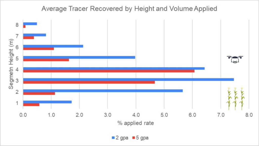
Overall, the volume applied had a significant impact on drift, where the 2 gpa treatment resulted in an average increase of 1.6 % applied rate ac-1 (44% difference: Table 8) versus the 5 gpa treatment.
Volume Applied (gpa)
Avg. % Applied Rate ac-1
Significance
2
3.6
A
5
2.0
B
Table 8- The volume applied had a significant impact on the amount of the PTSA recovered.
As with the Mylar samplers, there was a “field effect” where the field had a statistically significant impact on the amount of tracer recovered (Table 9). However, unlike the Mylar samplers in the crop, more tracer was recovered in field 2 (average increase of 3.2 applied rate ac-1 or a 67% difference) than in field 1.
Field
Avg. % Applied Rate ac-1
Significance
1
1.4
A
2
4.2
B
Table 9- The field location had a significant impact on the amount of PTSA recovered.
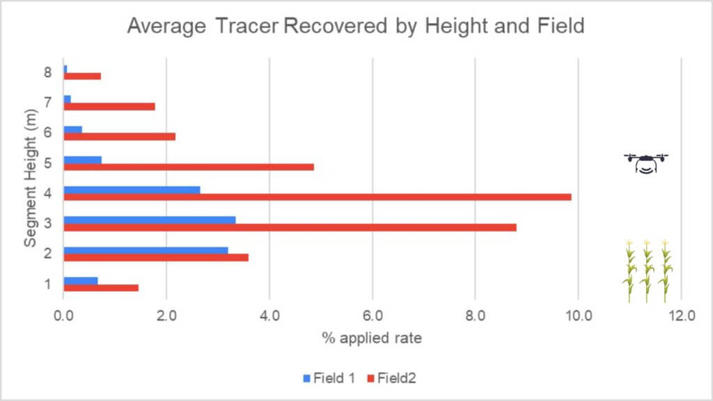
The pattern of deposition by height was similar across all treatments. For context, note that the first 2.5-3 m of string were within the corn canopy and drone altitude was approximately 5 m off the ground (2 m over the tassels) per Figure 4 and 5. The differences were only statistically significant in field 2 (Table 10) where an average 33% applied rate ac-1 was intercepted compared to 11% in field 1.
Figure 4- Average PTSA recovered (% applied rate ac-1) by height and field.Figure 5- Average PTSA recovered (% applied rate ac-1) by height and volume applied.
Height (1m segment in m from ground)
Field 1: Avg. % Applied Rate ac-1
Sig.
Field 2: Avg. % Applied Rate ac-1
Sig.
8
0.7
A
1.5
C
7
3.2
A
3.6
BC
6
3.3
A
8.8
A
5
2.7
A
9.9
A
4
0.7
A
4.9
AB
3
0.4
A
2.2
BC
2
0.1
A
1.8
C
1
0.1
A
0.7
C
Total:
11.2
–
33.3
–
Table 10- The average amount of PTSA recovered by height for field 1 and field 2.
The volume applied had a significant effect on the total PTSA tracer detected in both fields, with an average 4.4% applied rate ac-1 more (a 59% difference) recovered in the 2 gpa treatment (Table 11 and Figure 5). Separated by fields, the 5 gpa treatment had an average 1.4% % applied rate ac-1 more (a 77% difference) in field 2 and the 2 gpa treatment had an average 2.8% % applied rate ac-1 more (a 76% difference) in field 2.
Volume Applied (gpa)
Field 1: Avg. % Applied Rate ac-1
Sig.
Field 2: Avg. % Applied Rate ac-1
Sig.
2
2.2
A
5.0
A
5
0.7
B
2.1
B
Table 11- The volume applied had a significant impact on the amount of PTSA recovered.
Mass Balance Accounting
It is never possible to entirely “close mass” in spray studies because there are other surfaces (e.g. leaves) within the vertical profile that intercept spray, as well as off-swath deposition and the ground itself (not measured in this study). Nevertheless, the exercise does allow us to estimate and compare how much spray was captured and how much remains unaccounted for (Table 12). We see that the 2 gpa treatment in field 1 had the highest unaccounted-for fraction, and on average we were able to account for an average 53% of the applied rate ac-1 in this study.
Field (Volume in gpa)
Coverage: Avg % Applied Rate ac-1 (A)
Drift: Avg % Applied Rate ac-1 (B)
Total % Detected (A+B)
Unaccounted Fraction [100-(A+B)]
1 (5)
51
5
56
44
1 (2)
26.5
17
43.5
56.5
2 (5)
30
24
54
46
2 (5)
19.5
40
59.5
40.5
Table 12- Closing mass using % PTSA detected on in-canopy samplers and on drift collectors.
RPAS and ground rig coverage – Water Sensitive Paper
The depth of the sampler had a significant effect on the overall average % area covered at all depths (Table 13). However, there was no significant difference at the two lower depths for deposit density (Table 14). In both cases, the negative linear relationship between coverage and sampler depth corresponds closely to the PTSA recovered on the Mylar samplers (see Table 3).
Sampler Depth
Avg. Coverage (% Area)
Significance
Top
2.80
A
Middle
1.28
B
Bottom
0.62
C
Table 13- Overall average % coverage by sampler depth.
Sampler Depth
Avg. Coverage (Deposits cm-2)
Significance
Top
44.5
A
Middle
17.9
B
Bottom
7.2
C
Table 14- Overall average deposit density by sampler depth.
The sampler orientation had a significant effect on both overall average % area covered (Table 15) and deposits cm‑2 (Table 16).
Sampler Orientation
Avg. Coverage (% Area)
Significance
Adaxial
3.03
A
Abaxial
0.12
B
Table 15- The orientation of the sampler had a significant effect on the average % area covered.
Sampler Orientation
Avg. Coverage (Deposits cm-2)
Significance
Adaxial
43.5
A
Abaxial
3.1
B
Table 16- The orientation of the sampler had a significant effect on the average deposit density.
The treatment had a significant effect on the overall % coverage (Table 17) with the overhead broadcast condition covering an average 3.31% more sampler surface (a 60% difference) compared to the next highest treatment value. The directed application delivered a significantly higher 67 deposits cm-2 (a 72% difference) compared to the next highest treatment value (Table 18).
Treatment (gpa)
Avg. Coverage (% Area)
Significance
Broadcast (16.7)
5.91
A
Directed (20)
2.32
B
Drone (5)
1.34
BC
Drone (2)
0.55
C
Table 17- Overall average % coverage by treatment.
Treatment (gpa)
Avg. Coverage (Deposits cm-2)
Significance
Broadcast (16.7)
92.6
A
Directed (20)
25.8
B
Drone (5)
22.9
B
Drone (2)
5.9
B
Table 18- Overall average deposit density by treatment.
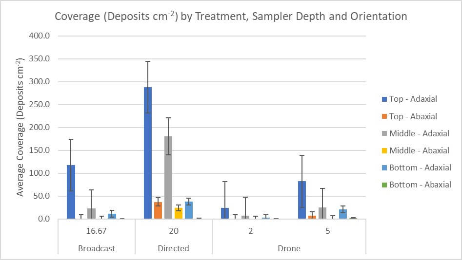
When we increase resolution to include sampler orientation, we see high standard errors typical of the variability inherent to spray coverage analysis (Figures 6 and 7). The broadcast treatment had the highest average adaxial % area coverage and the second highest average deposit density. The directed treatment had the second highest average adaxial % area coverage and the highest average deposit density but had the highest overall average coverage on the abaxial samplers. RPAS coverage on all samplers was lowest overall and was relative to the volumes applied.
Figure 6- Coverage (% area) by treatment, sampler depth and orientation.Figure 7- Coverage (Deposits cm-2) by treatment, sampler depth and orientation.
Focusing on RPAS treatments, the orientation of the sampler significantly affected coverage (Tables 19 and 20).
Sampler Orientation
Avg. Coverage (% Area)
Sig.
Avg. Coverage (Deposits cm-2)
Sig.
Adaxial
1.1
A
11.6
A
Abaxial
0.0
B
0.4
B
Table 19- RPAS (2 gpa) coverage by sampler orientation.
Sampler Orientation
Avg. Coverage (% Area)
Sig.
Avg. Coverage (Deposits cm-2)
Sig.
Adaxial
2.5
A
47.3
A
Abaxial
0.2
B
7.5
B
Table 20- RPAS (5 gpa) coverage by sampler orientation
Continuing to focus on the RPAS treatments, the depth of the sampler had a significant effect on overall average coverage at both 2 gpa (Table 21) and 5 gpa (Table 22). Just as with the average % applied rate ac-1 (included here for comparison), the overall average coverage on the top adaxial sampler was significantly higher than the other two depths for % area covered and deposits cm-2.
Sampler Depth
Avg. Coverage (% Area)
Sig.
Avg. Coverage (Deposits cm-2)
Sig.
Avg. % Applied Rate ac-1
Sig.
Top
1.2
A
12.8
A
7.5
A
Middle
0.4
B
3.9
B
3.8
B
Bottom
0.1
B
1.3
B
1.7
B
Table 21- Coverage on the top sampler was significantly different than other depths at 2 gpa.
Sampler Depth
Avg. Coverage (% Area)
Sig.
Avg. Coverage (Deposits cm-2)
Sig.
Avg. % Applied Rate ac-1
Sig.
Top
2.1
A
48.3
A
9.2
A
Middle
1.1
B
17.6
B
5.8
B
Bottom
0.9
B
16.4
B
2.3
B
Table 22- Coverage on the top sampler was significantly different than other depths at 5 gpa.
Comparing data from WSP to Mylar Samplers
There was a correlation between the % area coverage detected using WSP and the tracer recovered from the Mylar samplers. Deposit density provides valuable information about the distribution of spray over the target surface but does not always correlate with % area covered, and it is therefore omitted from this comparison. When we plot the average % area covered from the adaxial WSP against the average % applied rate ac-1 from the Mylar samplers, we see the same near-linear pattern of decay with depth (Figure 8).
Figure 8- Average coverage from adaxial samplers plotted by depth and volume applied show similar coverage patterns.
If we assume each top, adaxial sampler (irrespective of sampler material) represents the highest degree of coverage, we can assign it a value of 100% and index the data to this value. This allows us to visualize and compare the two sampler types directly (Figure 9) and illustrates similar relative coverage, but perhaps a greater rate of decay for the WSP.
Figure 9- Average coverage from adaxial samplers plotted by depth and volume applied show similar coverage patterns. Normalized to top sampler.
Net Revenue and Disease Pressure
Crops were harvested at the R4 stage of development. There was no disease pressure detected in any field and no clear impact of application method on net revenue (Figure 10). Results based on the following formula: (CAD $/ac) = (Seed Yield × Corn Sale Price) – Drying Cost. No conclusions regarding efficacy can be drawn from this data.
Figure 10- Net Revenue (CAD $/ac) by field and treatment.
Key Observations
Water Sensitive Paper (WSP) measurements of percent area covered (% area) and deposit density (deposits cm-2), and Mylar samplers measuring mass deposit (% applied rate ac-1), revealed similar coverage patterns, making both samplers viable methods for RPAS coverage analysis. These are complimentary methods that reveal different aspects of coverage. When possible, they should be used simultaneously to produce a more complete analysis.
RPAS and conventional overhead broadcast applications produced similar deposition patterns in the corn canopy: A negative linear relationship between coverage and adaxial sampler depth was observed for most treatments (r2=0.997) and abaxial coverage was very low or more often, nonexistent. Further, overall coverage shared a direct relationship with volume for RPAS and conventional overhead broadcast applications.
Directed applications in this study employed a finer spray quality, released laterally from within the canopy. This produced a different coverage pattern than the RPAS and overhead broadcast applications. Per WSP, this treatment resulted in the highest overall deposit density and was the only treatment to produce significant deposition on abaxial surfaces.
For RPAS, spray coverage was significantly reduced by -58% (based on avg. applied rate ac-1), by -59% (based on avg. % covered) and by -74% (based on avg. deposits cm-2) and drift was significantly increased by +73% for the 2 gpa treatments versus the 5 gpa. We attribute this primarily to drone travel speed, which increased from 3.3 m/s at 5 gpa to 7 m/s at 2 gpa. For context, and with certain exceptions, travel speed shares a negative relationship with spray coverage and a direct relationship with drift in airblast and field sprayer applications.
There was a “field effect” where field 2 had lower overall RPAS coverage for both 2 and 5 gpa treatments. Compared to field 1, by -28% for the 2 gpa treatment, and by -41% for 5 gpa. Average drift increased by +76% for 2 gpa and by +77% for 5 gpa. We attribute this to the significantly higher wind conditions in field 2.
Given the lack of disease pressure in the two fields, and the lack of any significant difference in revenue by treatment within each field, efficacy is inconclusive. This study represented only two of eight fields in a larger RPAS efficacy trial where five locations had disease pressure high enough to rate. Preliminary results suggest that Tar Spot control from a 5 gpa drone application may be comparable to that of a 16.7 gpa overhead broadcast application from a field sprayer (data not shown).
Summary
Drone and conventional overhead broadcast treatments deposited spray in a similar pattern (a negative linear relationship with canopy depth and very low or no abaxial coverage), irrespective of the method used to analyze coverage. RPAS produced significantly lower coverage than the conventional overhead broadcast treatment, which is attributed primarily to the low volumes employed, per the direct relationship between volume applied and overall coverage (up to some point of diminishing return). High ambient windspeed significantly increased drift in both the 2 and 5 gpa conditions and reduced spray coverage. High travel speeds (required to apply 2 gpa) likely contributed to the significantly increased drift and reduced coverage in that treatment versus 5 gpa. For the use cases explored in this study, low volumes and high travel speeds are not advisable for RPAS, particularly in high wind conditions. Future work separating the travel speed and ambient wind speed variables would clarify their relative influence on RPAS drift and coverage.
This video presentation is covers the highlights of the study. And disregard the verbal slip-up: we didn’t travel 110 mph.
We were long overdue for a new classic rock parody, so we decided to re-tackle one of the greatest rock ballads ever written. With the ongoing success of drop pipes (aka drop arms, drop legs, etc.) in corn, we’re promoting directed spraying in verse.
If you’d like to read more about the research, check out this article, and this one too. Farmtario also wrote a nice summary from one of our 2022 demos.
So, this was a tough one, but we feel good about how we laminated a new message over Zeppelin’s tricky cadence and rhymes. It helps if you play the actual song as you read. Rock on:
There’s a grower who’s sure all corn glitters like gold and he’s spraying from seven to seven.
When he’s done, then he knows that the products he chose will handle the pests that he sprayed for.
Ooh ooh ooh ooh ooh And he’s spraying from seven to seven.
He sees signs on them all but he wants to be sure ‘cause he knows bug poop means that they’re feeding.
So, he stops for a look spits and wipes as he should sometimes all of his thoughts are misgivings.
Ooh, it makes him wonder Ooh, it makes him wonder
There’s a feeling he gets when the silks seem too wet and his scouting is slowly revealing.
In his fields he has seen in the irrigation rings that tarspot’s in the plot where he’s standing.
Ooh, it makes him wonder Ooh, it really makes him wonder
Maybe he sprayed the corn too soon Or too late, it could be too ‘cause the timing defies common reason.
And he goes back in the dawn to see what else has gone wrong and his checks echo pests that he’s after.
Oh whoa-whoa-whoa, oh-oh
If there’s cutworm in your corn row, don’t be alarmed now. It may have been coverage or timing.
But there’s a new way, you can spray now, and in the long run there’s time to change the for the next season.
And it makes him wonder Oh, whoa
Overhead spraying is a no-go in case you don’t know drop pipes are calling you to try them.
Diseases come in when the wind blows but did you know drop pipes cover stalks from end-to-end.
So, as you drive on down the row overhead spray just won’t go deep into targets, we all know are hard to hit deep down below.
Next year he can still have gold. Using drop pipes isn’t hard. Coverage will come to him at last.
Quick to mount, one and all, yeah They barely rock as sprayers roll.