Category: Rates and Calibration

For basics category

How to Properly Set Up a Crop Sprayer
Article reprinted with kind permission from an original article written by Oliver Hill in the February, 2017 edition of Farmers Weekly. Photos ©Kathy Horniblow.
Crop spraying is one of the most important and highly skilled jobs undertaken on any arable farm, but it is facing increased public scrutiny. This is why it is vital that the kit you use as a means to apply pesticide to crops is in prime working order and is set up correctly to deliver the product safely and accurately to its target. Optimum sprayer set up will help to maximize the efficacy of applied products, reduce spray drift and keep machinery in good condition.
For this best practice guide to sprayer set up, Farmers Weekly teamed up with former Farm Sprayer Operator of the Year Iain Robertson. Mr. Robertson is assistant arable farm manager at David Foot Ltd, a 2,200ha mixed farm south of Dorchester in Dorset, growing wheat, barley, beans, oilseed rape and maize as forage for the farm’s three dairy herds. The machine used for this guide is a Bateman RB26 self-propelled sprayer and while most of these checks and tests are universally applicable to all sprayers, it is also important to refer to the handbook of the manufacturer of your specific machine.
Watch the video tutorial with Mr. Robertson and then see the step-by-step guide below for more detail.
Pre Start Checks
Before firing up the engine, the first thing to do is your pre-start checks – that means checking your machine’s vital fluids like fuel, hydraulic oil, hydrostatic oil, engine oil and coolant levels. If yours is a self-propelled sprayer, chances are you’ll need to get up on to the back of the machine to check some of these.
“While I’m up on the back of the sprayer I also have a quick look in the top of the tank to make sure that it is nice and clean and the tank rinse nozzles have worked properly – cleanliness is next to godliness,” says Mr. Robertson. Next, move on to the tires. Use a pressure gauge to check all tires are at the correct pressure and refer to the manufacturer’s guidelines. If you’ve got a trailed sprayer, don’t forget to check the tractor tire pressures as well.
Aim for tires to be run at the lowest pressure recommended for the load to be carried. This will help with boom height and stability and also helps tires act like a shock absorber to ride out bumps. If using a trailed sprayer, use a spirit level to ensure that the drawbar is level. Mr. Robertson says he tries to work around the machine in a methodical, clockwise manner to ensure that he doesn’t miss anything.
Coming to the pumps, check that they have got enough oil, check that any tool boxes have enough spare parts and any equipment needed and make sure you are carrying a spill kit with absorbent granules and a spade in case the worst happens and there is a spillage. Make sure all parts are lubricated daily and that any grease nipples are cleaned before and after use to avoid them collecting dirt and blocking.
Check all hydraulic hoses, spray lines and air lines for any signs of wear that could result in problems while operating.
It’s best to run the sprayer at a minimum of 5 bar to check for leaks. Also check the spray tank is fixed down securely, all straps and bolts are tight.
Boom checks
Once opened out, check the boom has good movement in the x- and y-axis. All machines are different so check with your manufacturer as to how the boom is set up. Mr Robertson’s Bateman has tie rods and stock bots that can be adjusted to set the boom up to ride well.
Check the tie rod nearest the back of the machine is slightly loose when moving and that the front rod is tight. Next, check for up and down movement by gently pushing the boom down by about 50cm and letting go. The boom should return to the central position without too much bouncing around.
“We want a little bit of movement but not excessive so that you can ride over the bumps as you go along without over- and under-dosing the crop,” says Mr. Robertson. Boom height is one of the most critical factors when spraying and the ideal height is 50cm above the crop. One of the easiest ways to work this out is by using a cable tie that is cut off at the correct length to use a visual aid from the sprayer cab.
Don’t forget to measure from the tip of the nozzle to the crop, not the spray line.
Good sprayer cleanliness is important, so make sure the system is rinsed through at the end of each day with clean water to make sure there’s no residue left in the boom. If your machine’s boom doesn’t have recirculation, remember to take the end caps off occasionally and flush out the whole boom.
Nozzle checks
Check that the nozzles are aligned both vertically and horizontally, according to the NSTS guidelines. Loosen clamps to adjust any nozzles that need realignment.
Check the nozzle output at least twice a year by running the sprayer with clean water at 3 bar pressure. Time the output of each nozzle for 30 seconds. If nozzles have been used previously, it’s best to check their output against that of a new pair. Mr Robertson advises using a measuring cylinder rather than a jug to measure the flow rate as a jug is less accurate “because you get a bigger variation over the wider surface area”.
With an 03 nozzle running for one minute at 3 bar pressure, the output should be 1.2 litres/minute as a rule of thumb but refer to the nozzle manufacturer’s output chart for the expected flow rate. “An easy way to remember this is: at 3 bar your nozzle size multiplied by four will give you your target litres/minute output. It works for all nozzle sizes.” If the output varies more than 4% of the average, or if the spray pattern visually doesn’t look correct, you need to change the nozzle set.
After checking the output, cross-reference this figure with the rate controller – you may need to adjust the flow figures to ensure that the two correlate. If a nozzle becomes blocked while spraying, Mr. Robertson says he will swap it for a new one and then clean it later using a toothbrush or airline. Never blow through a nozzle with your mouth.
Nozzle choice
The choice of nozzle is highly dependent on the sort of job you’re doing. “Timing is crucial but using the right nozzle at the right time will make the job so much easier, cut drift and mean that you’re getting more of the product where you want it to go. If you aim at it you will hit it,” says Mr. Robertson.
His nozzle of choice is an 03 size and he prefers to use the Defy 3D nozzle alternated forwards and backwards across the boom for pre-emergence work and T0 applications as well as the T3 ear spray. “In less than optimum conditions I may prefer to use the Amistar/Guardian Air, a fine induction nozzle. I would use this at T1 and T2 and also in sub-optimum conditions.” This nozzle has a 3-star Local Environmental Risk Assessment for Pesticides (LERAP) rating and is 75% drift reducing.
A water volume of 100 litres/ha is a good rate for spring fungicide application. It provides enough coverage for good disease control and allows maximum efficiency from the sprayer.
Forward speed
The third and final part of reducing spray drift is forward speed. Depending on nozzle size and water volume, aim to travel at 12kph.
Mr Robertson says he finds that this speed gives a good overall output and means you don’t get shadowing or turbulence behind the machine.
Tips and tricks
One of the biggest risk of contamination is at fill up. “A fantastic, cheap trick that I learned through Farm Sprayer Operator of the Year is to take a 200 litre plastic drum and cut it in half to create two drip trays to catch any spillages under the induction hopper and the tank overfill.” This eliminates point source contamination, he says.
“Finally, there’s a plethora of information out there on the internet, loads of good apps to download. The technology is there to help us do the best job possible and make our job as safe as possible.”
May 20, 2026

Alternate Row Spraying

Alternate Row (aka Alternate Row Middle [ARM]) spraying is an application method where the air-assist sprayer does not pass down every alley during an application. The sprayer operator is relying on the spray to pass through one or more rows and provide acceptable coverage to the entire canopy (or canopies) on a single pass.

Some state agencies promote this spraying strategy to various degrees, and many sprayer operators (whether they admit it or not) have used this method of spraying. I have advised it myself for very young and/or very sparse vineyard and orchard plantings, but never without confirming coverage. When I tell operators that I have serious reservations about alternate row spraying, they defend it. Here are the most common justifications I’ve heard over the years, and my response:

Justification	Reply
“I do not have enough spray capacity to spray every row when time is short.”	You need more sprayer capacity. Get another sprayer so you can get spray on in time or invest in a multi-row sprayer is possible.
“ARM spraying saves money and reduces environmental impact because I use less pesticide.”	Technically, if you travel every second row with a sprayer calibrated to travel every row, you have indiscriminately reduced your carrier and chemical inputs by half (or more). Without close monitoring you may compromise your efficacy.
“I only perform ARM spraying early in the season when canopies are empty, or only on young plantings.”	I grudgingly grant this one as long as coverage is closely monitored. I’ve prescribed it myself in young or sparse plantings where I couldn’t get the sprayer output low enough to prevent drenching the targets.
“The spray plume in the alley beyond the target row must mean the spray is providing adequate coverage. More is better!”	If the spray is blowing through the canopy, it isn’t landing in the canopy. Further, if the air speed/volume is too high, droplets can ‘slipstream’ past the target without impinging on them. I’ve removed water-sensitive paper from canopies with barely any spray on them despite the plume in the downwind alleys. It looks like a magic trick, albeit an unhappy one.
“Uncooperative weather doesn’t always leave me enough time to spray the entire crop, and it is the lesser of two evils to spray alternate rows than not at all. I’ll make sure I come back to spray the other rows later.”	Choosing to do half a job requires an understanding of the products’ mode of action. If you are spraying an insect at a particular stage of development, there’s no “coming back later” to get that generation – if you missed, your window has closed. If it’s a protective fungicide that offers no kick-back, then once the disease has infected tissue, the damage is done. Get the spray on as best you can, but if it washes away before it has a chance to dry sufficiently, be prepared to reapply at the earliest opportunity as long as the label allows it.
“ARM has always worked in the past.”	Would you mind picking my lotto numbers for me? You’re a very lucky person!

My reservations about ARM spraying come from published research and personal experience that show that coverage is almost always compromised when spraying from one side of a canopy. The spray must pass through the canopy to reach the far side, and the canopy filters droplets from the air as it passes through. This reduces the number of droplets available to cover the far side. In addition, high velocity spray will create “shadows” where any targets on the immediate far side of a leaf or branch become shielded and receive little if any coverage. Further still, fine droplets slow quickly as they leave the nozzle and take a long time to settle. As the entraining air slows and becomes erratic, the droplets float and change course, making their behaviour hard to predict.

The cumulative impact can be seen in this infographic I built in 2016. The orchardist was a dyed-in-the-wool ARM applicator and he was resistant to driving every row because it took so much time. I wanted to show that he could claw back some of the lost time by spraying less pesticide every row versus his current volume every second row. He would need fewer refills, and save a LOT of unnecessary pesticide. The water sensitive paper does the talking, and while I’d like to think I’ve convinced him, I’ll bet he’s still out there dicing with fate.

A very popular argument in favour of ARM spraying comes from orchardists that are shifting from semi dwarf to high-density plantings. They ask “How it is different to spray a four foot diameter tree from one side compared to an eight foot diameter tree from both sides”?

Well, we know coverage is reduced as a factor of distance. Spraying from one side gives a single opportunity to cover the middle and far side of a canopy, whereas spraying from both sides provides an opportunity for an overlap in coverage. Essentially, the centre of a canopy receives the cumulative benefit of two sprays. Coverage is therefore always improved when spraying from both sides, period.

Spraying from one side gives a single opportunity to cover the far side of a canopy. However, spraying from both sides provides an opportunity for an overlap in coverage. In other words, the centre of a canopy receives less spray than the outside, but is essentially sprayed twice resulting in a compounding effect.

Why, then, do some sprayer operators claim that alternate row applications work? Because sometimes, they do! Just because coverage is reduced doesn’t mean it isn’t sufficient to protect the crop. It simply means that the potential for poor coverage and reduced dose is dramatically increased by alternate row applications. A sprayer operator might perform alternate applications successfully for years before conditions conspire to defeat the application: unfavourable wind, poor timing, increased pest pressure, poor pruning practices, excessive ground speed, high temperatures, low humidity, insufficient spray volume, and several other factors might occur simultaneously and reduce coverage below a minimal threshold for control. This confluence of bad luck may not happen the first year, or the second, but eventually…

Product failure isn’t the only concern. Repeated reduced dosages may play a role in developing resistance. In those situations where the operator recognizes insufficient coverage, they may have to spray more often to compensate, negating any savings in time or product. Reduced dosage is a common error when a sprayer operator elects to use ARM.

If you still aren’t convinced, at least perform alternate row spraying the “right” way. Here are three situations that I’ve heard operators refer to as alternate row spraying. Situation 1 is most common, but to my mind only Situation 2 would be considered acceptable. Even then, confirming coverage is a must.

Situation 1:

The sprayer has a typical calibration for spraying every row, but only drives alternate rows. The first application (solid line) covers different rows from the second application (broken line). The operator will claim to spray more frequently, but generally does not perform the second application unless there is high pest pressure. The result is half-a-dose per hectare per application.

Situation 2:

The sprayer is calibrated for double output compared to a typical every-row situation, and the operator drives alternate rows. The result is that the hectare gets the whole dose per application, but coverage is always inconsistent.

Situation 3:

Since the sprayer will only drive alternate rows, the operator mistakenly sets the sprayer to emit half the output compared to a typical every-row situation. The first application (solid line) covers different rows from the second application (broken line). The result is a quarter-dose per application, and if the operator chooses to spray a second time, the hectare will only ever get half-a-dose. Yes, this happens.

So, my final word on alternate row applications is that they should be performed with extreme caution. I’ve used them myself in early season applications in new plantings, but never without confirming coverage with water-sensitive paper, and never in conditions that might further compromise coverage to the point that the application does not give control.

Caveat Emptor!

Well, I thought it was funny. My apologies to J. Luymes from British Columbia (pictured) and Obi Wan Kenobi (not pictured… or is he?)

May 20, 2025

Calibrating a Plot Sprayer for Airblast Crops
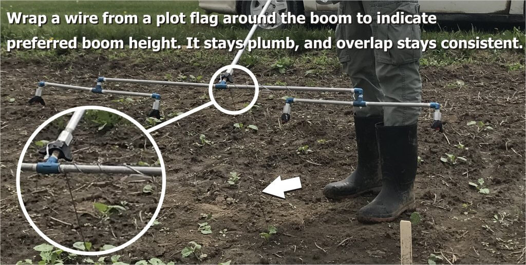
The calibration of handheld plot sprayers is an important part of agricultural research, and this article already covers all the bases… as long as you are spraying broadacre or row crops. But what happens when you are trying to emulate an airblast sprayer and treating a tree, bush, cane or vine?
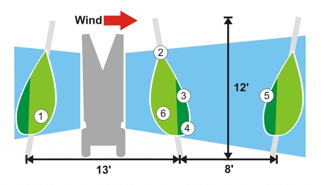
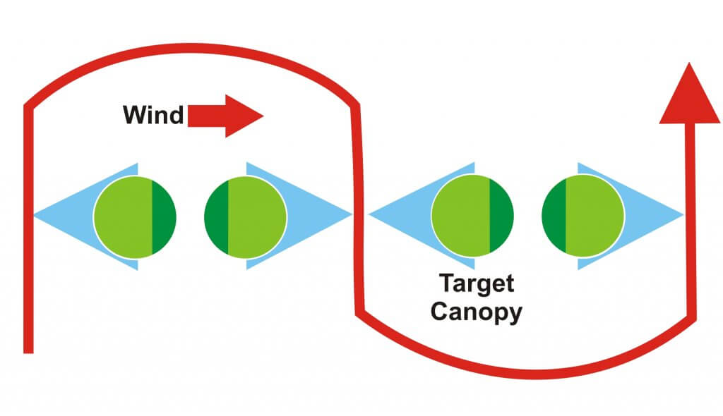
The key difference is that spraying a two dimensional area requires the operator to pass the boom over the target at a uniform height and pace to achieve consistent coverage. But, a three-dimensional target requires the operator to circle the target, or spray from both sides, until it has received the required dose (or volume).
In order to scale down a typical airblast carrier volume for small plot work, we need to know three things:
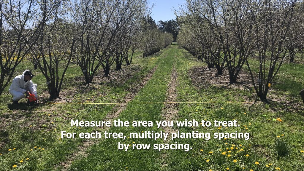
1. The area you wish to treat (e.g. bush, grape panel, tree, etc.), including it’s share of the alley (in m²).
2. The emission rate from the calibrated plot sprayer (in US gal./min.)
3. The airblast carrier volume you wish to scale down (e.g. L/ha).
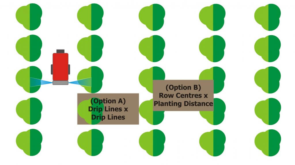
The illustration below shows two options for calculating the treated area. Option A requires you to measure from the outermost edges of the canopy (imagine if the canopy was wet and dripping – the dripline is that outermost point). It is less consistent than the preferred Option B, where the area is determined from row centres and planting distance.
Two options for scaling down an airblast carrier volume for small plot work. Both produce the same treated area, but Option B is the preferred method.
Use the average planting distance and row spacing in metres. For a panel of grapes, use the centre of each panel as the planting distance.
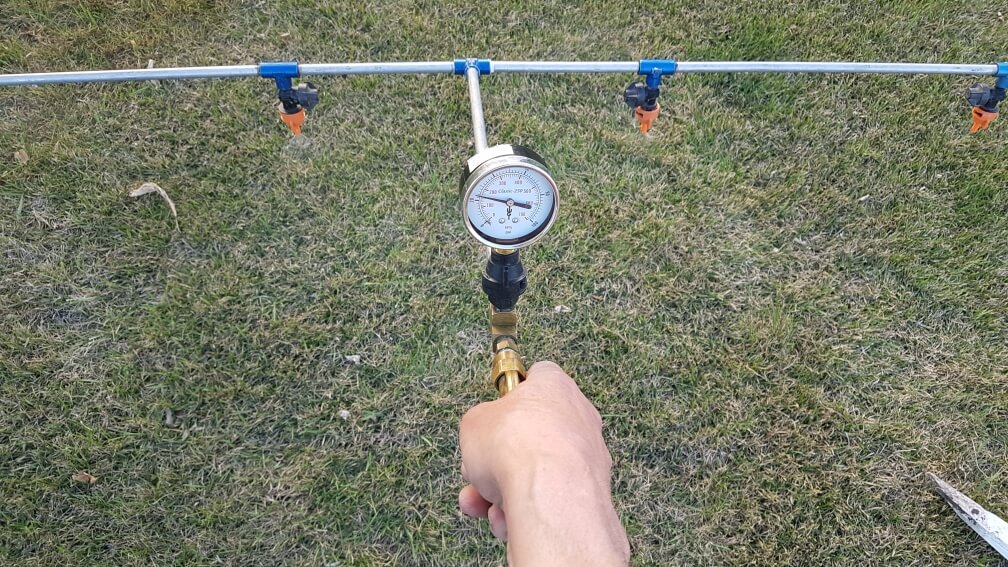
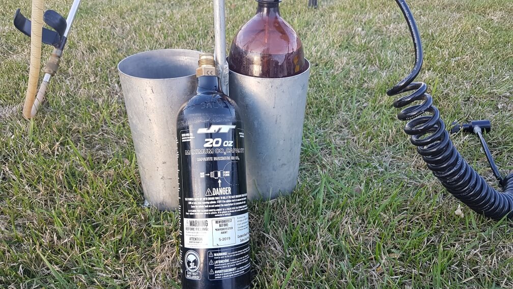
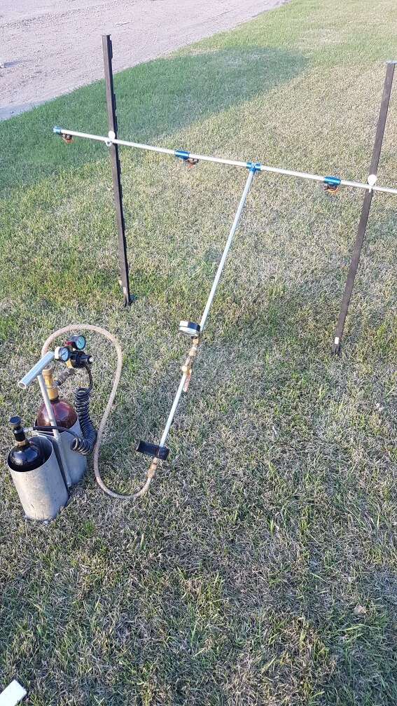
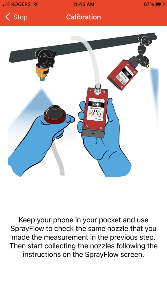
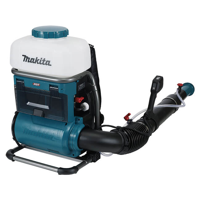
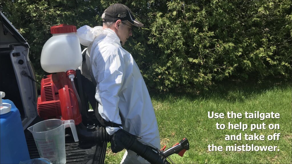
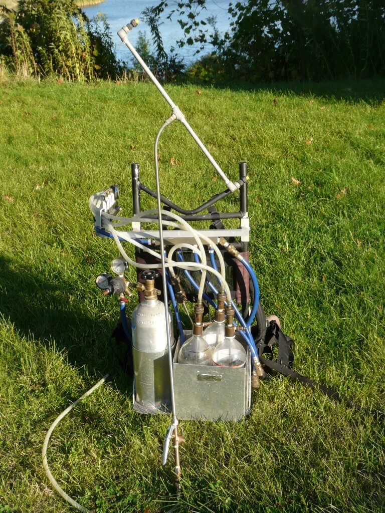
If you are using a CO₂ powered hand wand (preferred over a manual pump) with one or more hydraulic nozzles, then you can calibrate it using the methods in this article. There are battery-powered options from Jacto and Petra Tools, the latter offering a battery powered ULV system as well. Makita also has a battery entry (image below). However, if you are using a backpack mistblower, which better approximates an airblast sprayer compared to a hydraulic hand boom (see this article), it requires a different approach. Plus, you get to look like a Ghostbuster, which is a win in my book.
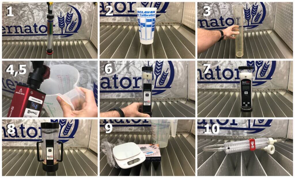
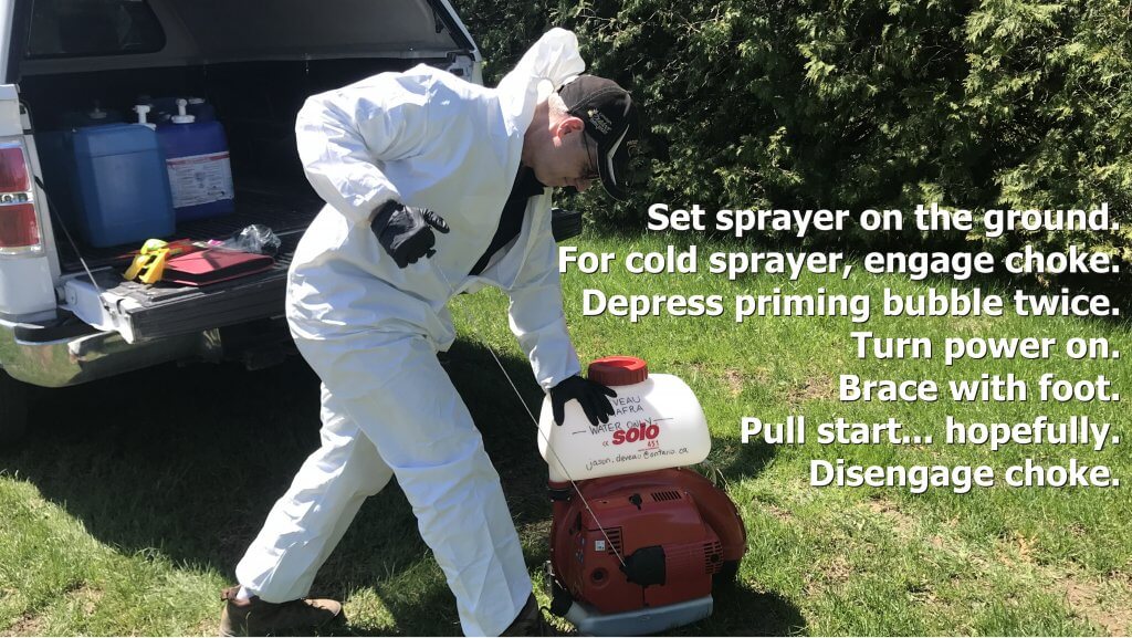
PM001GL201 – 40V max XGT Brushless Cordless 15L Backpack Mist Blower (8.0Ah x2 Kit)
Follow along in the following images as we explore how to calibrate a backpack step by step:
When transporting a mistblower, use a loop of nylon cord to secure the boom in an upright position.
For calibration, fill the completely empty sprayer with a known volume of water. If the boom is gravity-fed, be sure the feed valve is closed so the water doesn’t run out of the boom.
With the sprayer on the ground, brace it with your foot. Step on the metal frame, not the motor housing or tank. Follow the operating instructions to pull start the motor.
Being cautious of the hot exhaust, set the sprayer on a tailgate, or other elevated surface to facilitate strapping it on.
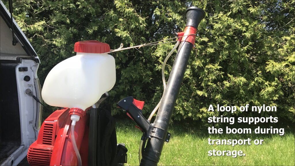
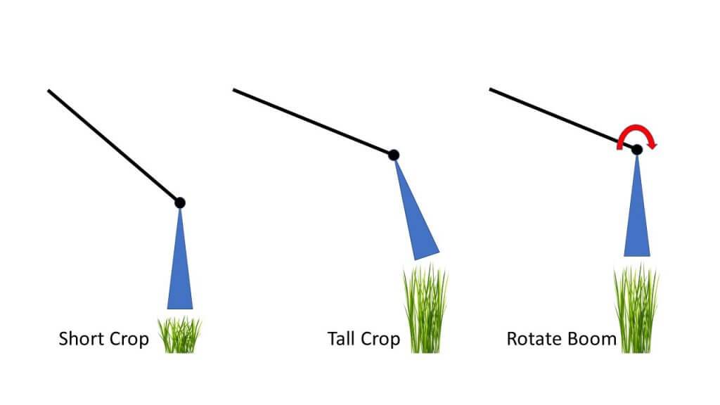
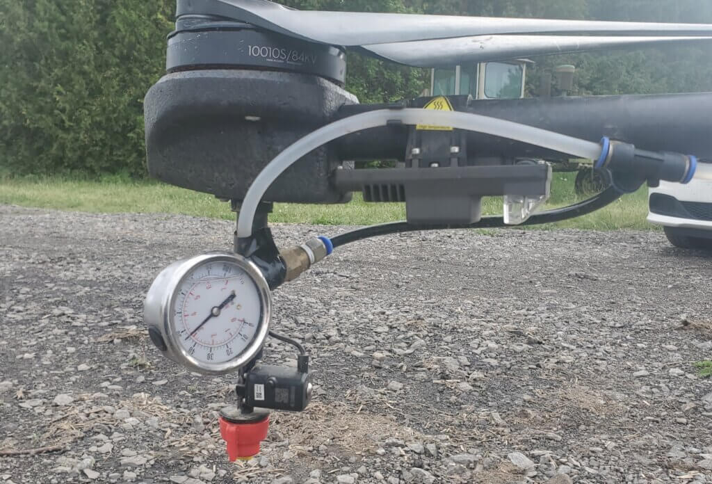
Be aware that most mistblowers use gravity to feed the spray mix from the tank to the boom. A pressure pump kit is recommended for applications where the spray tube is held upward more than 30 degrees to maintain a consistent discharge rate. A hip belt is also recommended to reduce fatigue. Examples are shown below are for Stihl-brand sprayers. Some may or may not require the pump (e.g. Tomahawk) but they are primarily intended for mosquito control and in that case a consistent rate over a vertical plane may not be as important.
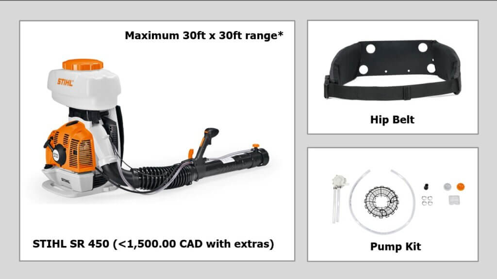
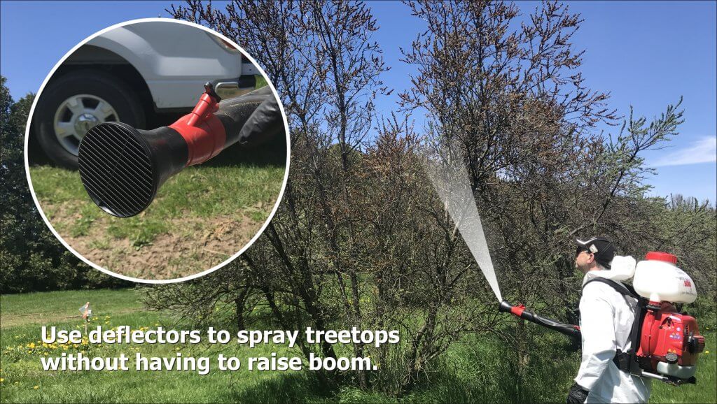
If your sprayer does not have a pump kit, pointing the boom upward will cause spray to slow or even stop. This greatly diminishes your ability to reach high targets and achieve consistent coverage. In this case, attach the deflector (which comes with the sprayer) before proceeding with the calibration.
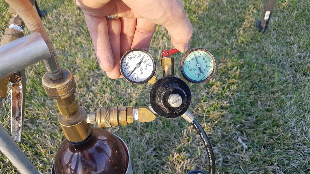
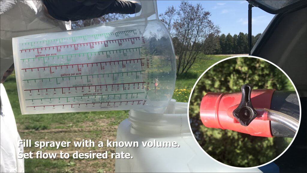
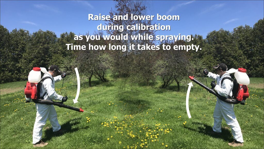
Deflectors angle the spray upwards without having to lift the boom. This is easier on your shoulder and keeps the rate consistent.
Set the flow rate to the preferred setting (usually a dial at the end of the boom), and using a stopwatch, time how long it takes to spray the entire volume. Be sure to move the boom exactly as you would when spraying the target, either side-to-side or up-and-down, to capture possible rate changes from the gravity feed. Convert the output to US gal./min.
When timing output, move the boom as you would when spraying the target.
Alternately, some people will stand on a bathroom scale with the backpack full. Then get off and spray for a period of time. Then get back on the scale. One millilitre of water weighs one gram, so you can calculate the flow from the weight difference.
Now you know the area and the emission rate. You should have a target carrier volume in mind (e.g. L/ha). Using the following example, let’s determine how long you need to spray the target:
A sample calibration.
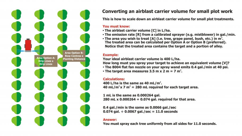
In this example, an ideal airblast Carrier Volume [C] for the orchard is 400 L/ha. We want to scale this down to determine the Volume for Treated Area [V]. First, divide [C] by 100 to convert it to 40 mL/m². Then, because in Canada our nozzles are in US units, we do an ugly conversion: Since 1 mL = 0.000264 US gallons, [C] becomes 0.0106 US gal./m².
The Treated Area [A] measures 3.5 m by 2 m = 7 m².
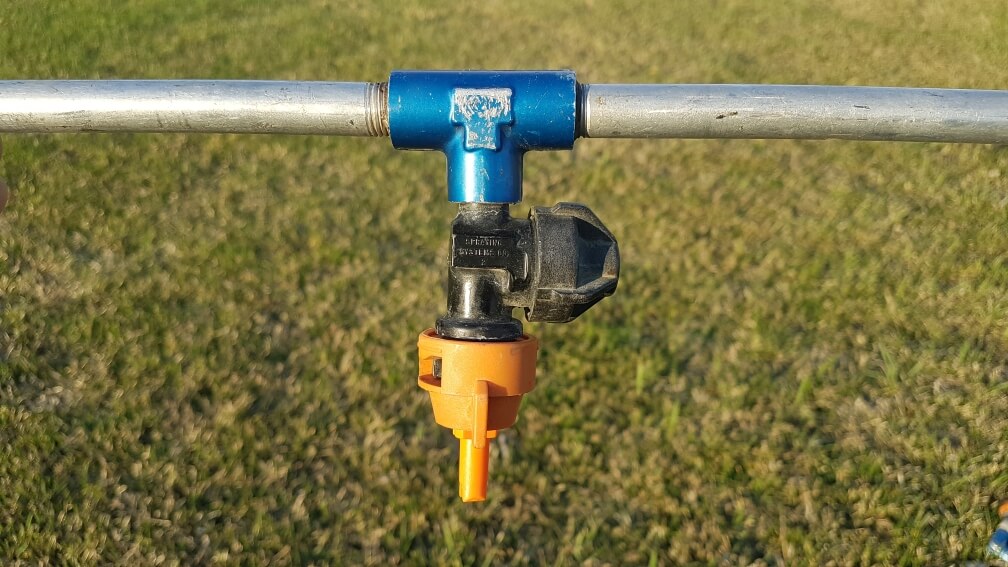
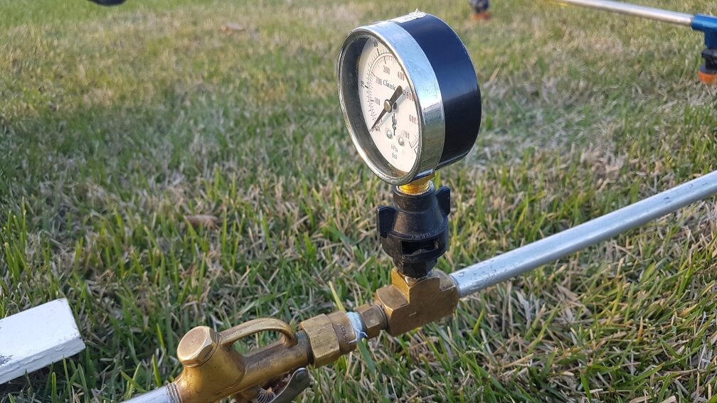
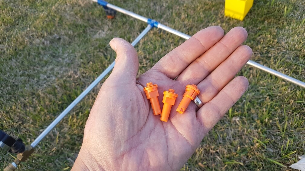
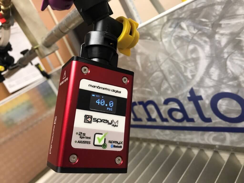
The Emission Rate [R] is the rate the plot sprayer sprays. While we prefer using a mistblower, many still use a hand wand with no air assist. In this case let’s suppose we are using a hand wand with two 8002 flat fan nozzles operating at 40 psi. According to our calibration, we confirm it sprays 0.4 US gal./min.
- [C](US gal./m²) × [A](m²) = [V] (US gal.)
- 0.0106 US gal./m² × 7 m² = 0.074 US gal.
We know we want to spray the target with 0.074 US gal., and we also know [R] which says our boom emits 0.4 US gal./min. We convert this to seconds by dividing by 60, so [R] = 0.0067 US gal./sec. From this we can calculate how long [T] we must spray the target.
- [V](US gal.) / [R](US gal./sec.) = [T](seconds).
- 0.074 US gal. / 0.0067 US gal./sec. = approximately 11.0 seconds.
So, we know that to spray the target with an equivalent 400 L/ha, we must achieve consistent coverage from all sides by spraying it for a total of 11 seconds. Pro tip: Always mix a little more spray volume than you will need to account for priming.
This is only one way to calibrate a backpack sprayer for spot spraying. If it’s isn’t quite what you need, check out these resources:
1. Calibrating a Knapsack Sprayer (www.weedfree.co.uk – 2008)
2. Don’t Overlook Backpack Sprayers (John Grande, Rutgers)
3. Hand Sprayer Calibration Steps Worksheet (Bob Wolf, Kansas State University – 2010)
4. Sprayer Calibration Using the 1/128th Method for Motorized Backpack Mist Sprayer Systems (Jensen Uyeda et al., University of Hawai’i – 2015)
Pro Tip: To maintain a consistent boom height without a wheel, coil a measured length of wire from a plot marker flag to guide you.
If the math is still giving you trouble, try our Ultimate Sprayer Calibration calculator.
May 12, 2023
Calibrating a Plot Sprayer
It’s the rite of passage of many agricultural summer students across the world: applying experimental treatments to field plots using a research sprayer. The results of these experiments may be the basis of new product use registrations, or provide clues into future scientific studies. Needless to say, the application method needs to be bullet proof to ensure the results are reliable. Here are a few guidelines, starting with some tips:
Pro Tips:
1. When assembling a hand-held boom, ensure the threads are properly sealed using Teflon tape. More or less tape can be used to create a snug fit at the right part of the thread rotation.
2. Choose nozzle bodies with diaphragm shutoff valves. These valves stop flow below 10 psi and prevent dripping of the nozzles after shutoff, without pressure drop during operation.
3. Avoid the use of older style “check-valve strainers”. Although these also prevent drips, they create a pressure loss of about 5 psi which creates uncertainty around the actual spray pressure.
4. Install a trusted pressure gauge on the handle of the sprayer in clear view for the operator. This provides important information. Don’t believe the gauge on the regulator. Ours, for example, is stuck at 30 psi.
5. For hand-held booms, rotate the booms so that the nozzles point down, for each application. Different size people or height of crops will change this angle and make accuracy more difficult.
6. Set the boom height so that you achieve 100% pattern overlap. This means that a nozzle’s pattern width should be twice the boom’s nozzle spacing. Boom height will be close to 50 to 55 cm above target, depending on fan. Too low, and the pattern may cause striping. Your supervisor will see that all year long and think of you.
7. You can test the spray pattern by applying water to a concrete pad. At the right boom height, the entire boom width should dry at a similar rate.
8. Install a visual guide for boom height. For example, place a wire flag at the end of the plot, at the correct height. This will provide a handy reference of boom height as your arms get weary. Or hang a wire, zip tie, or chain from a spot that doesn’t interfere with your spray pattern (thanks ACC).
9. Minimize weight by using smaller bottles of CO₂. We use 20 oz paintball bottles, they are much lighter, last long enough, and can be legally refilled with liquid CO₂ or topped up with gas from a nurse tank in the field.
10. Spray out leftover mix in a designated part of the plot area. Do not pour any mix on the ground. Please. Consider a biobed on your research farm.
11. When completing a treatment, spray the boom completely empty so air comes out of each nozzle. This provides certainty that the next liquid at the nozzles is from the next bottle, be it water or another treatment.
12. When spraying dose responses of the same product, always start with the lowest dose. Again, spray out in a designated place until the boom produces air, no need to flush.
13. Construct a boom hanger from electric fence posts and coat hangers. Nozzles face down and can be serviced. The boom should never lie on the ground.
14. Use nozzle screens to prevent time delays due to plugging. Usually 50 (blue) or 80 (yellow) mesh is sufficient. Any finer mesh may interfere with some dry formulations. Note: Beware old screens – ISO mesh colours have changed. Learn more here.
15. It’s very useful to apply research sprays with low-drift nozzles. Air-induction tips are most effective. These reduce drift, and are also closer to the commercial spray quality used by producers.
16. 01 size (orange) air-induced nozzles are available from Albuz (AVI Twin and AVI), Arag (CFA, CFAU, AFC), Billericay (Air Bubble Jet), Greenleaf (AirMix and TurboDrop XL), Lechler (ID3 and IDK). No other major manufacturer produces this small size of tips in air-induction.
17. 015 size tips (green) and larger are produced by the above, as well as Albuz (CVI Twin and CVI), Hypro (GuardianAIR or ULD) and TeeJet (AIXR, AI, and TTI), within both manufacturers listed in order of increasing coarseness.
18. Always carry several other nozzles of the same size and type already on the boom. Should a nozzle plug, replace it, don’t clean it. Clean it later.
19. If a nozzle plugs and there is no extra nozzle, use compressed air to clean it. Compressed air electronics cleaners are available in most electronic stores.
20. If a plugged nozzle can’t be cleaned, simply place it at the end of the boom and continue. Plot ratings and yields are usually taken from the centre. Remind your supervisor of this.

21. Always de-pressurize a sprayer before disconnecting any liquid hoses. You can’t rely on check valves. If two people work together, make sure you practice and communicate this with each other.
Calibration:
1. Assemble the sprayer and run water through it to ensure it’s free from silt or residue. Repair leaks.
2. Install nozzles and ensure none are plugged and the pattern looks good.
3. While spraying water, set pressure to what you intend to spray with. (Note: boom pressure will be lower than regulator (attached to CO₂ canister) by a few psi, hence the separate pressure gauge on the boom. Also note that the set pressure will always be higher when the system is at rest.)
4. Obtain four containers of similar size that can hold about 500 mL, and place on ground at nozzle spacing. Using stopwatch, emit spray directly into all four for a set time, say 30 s.
5. Expected spray volume at 40 psi: 01 tip, 380 mL/min; 015 tip, 570 mL/min; 02 tip, 760 mL/min. In other words, from a 2 L bottle you’ll not get much more than 30 s spray time from 4 tips.
6. Measure collected volume from four tips using the same graduated cylinder.
7. Repeat, for total of three times.
8. Average three reps for each nozzle and convert to mL/min. Make sure all nozzles are within 5% of the average flow. Replace those that aren’t or place worst offender on outside edge of boom.
9. Advance to “Calculations”, but be prepared to conduct another calibration
Now for the fun part.
Calculations
There are three options for applying the correct amount. We’ll be using metric in these examples:
1. Use the average nozzle flow from the calibration (mL/min) and the target application volume (L/ha) to calculate the necessary walking speed (km/h);
  
  or
2. Use the flow from the calibration and a set walking speed to arrive at an application volume;
  
  or
3. Use a set walking speed and a set application volume to calculate a required calibrated flow.
Option 1:
Walking Speed = (60*flow)/(Volume*nozzle spacing)
If your nozzle flow was 330 mL/min and you wanted to apply 100 L/ha using a sprayer with 50 cm nozzle spacing, your required walking speed is 60*330/100/50 = 3.96 km/h
Option 2:
Application Volume = (60*flow)/(Speed*spacing)
If your nozzle flow was 330 mL/min and you wanted to walk 5 km/h using a sprayer with 50 cm nozzle spacing, your application volume is 60*330/5/50 = 79 L/ha
Option 3:
Required flow = (Speed *Volume*spacing)/60
If your speed is 5 km/h and you wanted to apply 100 L/ha using a sprayer with 50 cm nozzle spacing, your required flow is 5*100*50/60 = 417 mL/min
If you selected Option 3, you now need to return to your sprayer and find a nozzle, or a pressure, that delivers an average of 417 mL/min. You can use math to get into the ballpark with the nozzle you already have:
New Pressure = (required flow/calibrated flow)²*calibrated pressure
If your required flow is 417 mL/min and the calibrated flow is 330 mL/min, and you calibrated at 30 psi, then you should be close to your required flow at (417/330)²*30 = 48 psi
Now, return to your sprayer, set the pressure to 48 psi, and confirm this estimate.
We use Option 3 when comparing nozzles of the same size but from different manufacturers. It’s not uncommon for these to have slightly different outputs. Rather than adjusting our walking speed slightly, which is very difficult to do accurately, we change pressure slightly so all nozzles produce the same flow. This is also useful when comparing water volumes by switching to a larger nozzle.
Travel Speed:
The last step is to confirm travel speed. Say you want to walk at 5 km/h. The best way to calibrate walking speed is to measure a known distance (m) in the field you’ll spray. Wearing the gear and carrying the sprayer you will use to spray, walk this distance. Use a wire flag to mark the start and end points; when the boom hits the flags, start and stop the timer. Repeat until comfortable.
Time needed to walk distance:
Time (s) = Distance *3.6/required speed
Say your walking distance is 10 m, and you need to walk 5 km/h.
10*3.6/5 = 7.2 s
A simple spreadsheet that can be used for the calculations can be found here.
Congratulations! You’re done. Happy spraying! Remember to not worry too much about a 5% deviation from your expected application. That’s definitely an acceptable error, as long as you don’t allow too many of those to add up.
Low Volume Research (Aerial)
Some product uses are by air, and the label volumes for those are often 30 to 50 L/ha. Registrants need to provide efficacy data at those volumes. Ground application can be accepted as a surrogate for aerial as long as the volumes are correct.
Since the spray nozzles aren’t typically available below the 01 (orange) size and if they are, they usually plug so easily and make such a fine spray that they’re frustrating to use. The alternative, to travel faster, is also problematic on research plots.
We recommend that Turbo TeeJet nozzles be used for this purpose. They produce such a wide fan angle that a 100 cm spacing is justifiable. Simply cap off every second nozzle body. Booms need to be elevated to ensure overlap, for uniformity. The value of the small nozzles and wider spacings is the low total application volume that is now possible.
The TT tips can also be used at fairly low spray pressures (say 20 psi) further reducing their output.
Spray Quality of TeeJet Turbo TeeJet (ASABE S572.1). This tip is available in smaller sizes and, due to its wide fan angle, can be used at 40″ (100 cm) spacing, therefoe applying low water volumes.
/
May 8, 2023
Adjusting Sprayer for Alternate Rows
An “Alternate Row Middle (ARM)” traffic pattern is where the sprayer passes down every second row. The intent is to improve work rate by cutting the driving time in half. The operator hopes to provide suitable coverage on both the sprayer-facing half of the canopy, and that half of the canopy facing the next alley. In our experience, this depends on sprayer design, and only works in very small/young plantings (or only for the first few applications of the season). Even then, the side facing the sprayer tends to get saturated in an effort to ensure a threshold dose reaches the far side. We’ve already captured the pros and cons of ARM in this article, and (spoiler alert) unless you’re using a wrap-around style design, it’s generally not the best approach for protecting an orchard, bush, cane or vine crop.
So why on Earth would we be testing it here?
We were contacted by an orchardist who planted a test block of Gala (est. spring, 2017) in an unusual way. He called it “V-Trellis Vertical Axis Cross”. Basically, he created an orchard architecture that only allowed equipment (e.g. platforms, sprayers) to pass down every second row. He figured it would save 35% of his labour costs. In the photo and illustration below, you can see the posts lean over the drivable alleys, creating a “V” shape.
So, given that he couldn’t fit a sprayer down every row, we had no choice but to try to optimize sprayer settings for ARM applications. Note the six numbers in circles in the above illustration. They indicate where we would eventually place water-sensitive papers to diagnose spray coverage.
Here are the settings the orchardist was using before we made any adjustments:
- Turbomist sprayer with 11 foot high tower
- Bottom-most nozzle was on and every second nozzle position skipped for a total of 5 nozzles active per side
- Nozzles were TeeJet ceramic disc-core. Top to bottom: D3-DC45, D3-DC45, D3-DC45, D3-DC45, D3-DC25
- 7 km/h (4.35 mph) travel speed per a speedometer app on a smartphone
- Tractor engine speed was 2,150 rpm (PTO was ~ 540 rpm)
- Fan set in low gear
- Pressure was 190 psi
- Ambient wind gusting to 8 km/h, temperature of 30°C, RH ~65%.
And here is a video of what the sprayer was doing before we changed any settings. This is a single upwind pass, and as you can see, the spray blew through at least five downwind rows. Obviously, this was far too much air and spray volume.
When we diagnose coverage in an every-row situation, we drive the alleys on each side of the target row (i.e. two passes). But, when diagnosing ARM spraying, we want to account for every drop of cumulative coverage from spraying upwind rows. So, we have to do three passes, as shown in the illustration below. In this top-down diagram, the sprayer travels the red line.
In order to establish a baseline, we diagnosed coverage for the original settings using water-sensitive papers in the six positions indicated above. We folded them in half, so a sensitive side faced each alley. We sprayed water and later digitized the cards to determine the percent coverage on the papers. Remember, if 80% of the cards receive at least 10-15% surface coverage and a deposit density of 85 drops per cm², it’s typically sufficient.
Here are our results, with percent area-covered indicated in each position, as well as a representative scan of one of the papers. There’s no need to provide deposit density, which after about 30% surface coverage cannot be reliably determined.
So, if the video doesn’t convince, then the papers certainly do: This was way too much air and spray mix.
Next, we performed a series of air adjustments using ribbons (detailed here and here) which led us to reduce engine speed from 2,150 rpm to 1,300 using the Gear-Up, Throttle-Down method. Then we used the OrchardMax calculator to establish an ideal spray volume and guide us to which nozzle rates we should use:
- Bottom-most nozzle was on and every second nozzle position skipped for a total of 5 nozzles active per side
- Top nozzle was TeeJet AITX8002, followed by TeeJet TXR80015, TXR80036, TXR80015, TXR80015
- 7 km/h (4.35 mph) travel speed per a speedometer app on a smartphone
- Tractor engine speed was 1,300 rpm (PTO was ~ 300 rpm)
- Fan set in low gear
- Pressure was 100 psi
- Ambient wind gusting to 4 km/h, temperature of 26.5°C, RH ~70%.
The following video shows the coverage from a single pass (to be clear, no extra upwind pass). We eventually did three passes to capture the cumulative coverage, just like with the first sprayer settings. This video simply serves to show how in ARM applications, the sprayer-facing side always looks much better than the side facing away. Also note how much quieter the sprayer is, as well as the reduced blow-through.
And here is the resultant, cumulative coverage from three passes. Once again, deposit density isn’t required as it exceeded our threshold in each position.
In the end analysis, we saved the grower ~30% of their spray mix, greatly reduced noise and spray drift, and still achieved suitable coverage in the target canopy. So, does this mean ARM applications are redeemed? We refer you, kind reader, to our introduction where we said ARM can work in young plantings and early season applications.
Note that the upwind side of the canopy received less coverage than the downwind side. As this new planting grows and fills, it’s going to be increasingly difficult to achieve sufficient coverage. Changes to the sprayer settings may be able to account for the imbalance, but they will also make the applications less efficient (i.e. more spray mix, more drift and coverage will still not be uniform). It remains to be seen if the spray inefficiency inherent to this orchard architecture is worth the estimated 35% savings in labour costs.
It’s an economic decision. We’ll see.
October 25, 2022