Tag: calibration

  • Optimizing a Greenhouse Vegetable Sprayer

    Optimizing a Greenhouse Vegetable Sprayer

    In April 2025 we visited Cedarline Greenhouses to assess their spraying methods. Our hosts invited us to examine their practices and then graciously agreed to let us share the process (and the results) so others could learn from the experience. Every greenhouse is different, but with a little imagination the process we used should translate to most operations. I want to be clear that this operation was already doing a good job before we showed up. It’s just easier for someone from the outside to scrutinize and find little things that might need tweaking. Let’s go through the steps we took that day.

    1. Measure the crop canopy and the planting architecture

    The objective of any spray application is to achieve sufficient coverage of the target with as little waste as possible. Achieving this goal means understanding the interaction between the sprayer, the spray droplets, and the crop canopy.

    Start by measuring the the planting architecture. These values allow us to calculate application rates and to calibrate the sprayer. Cedarline is a 16-acre pepper operation. The crops are strung vertically in double rows for a total canopy depth of about 1 m, leaving roughly 0.5 m clearance in the alleys. Spraying takes place while the crop is between 1.5 and 3.5 m high. Each row is 102 m long.

    2. Consider the target from the droplet’s perspective

    Stand between the rows and face the canopy. Where is your spray target relative to the nozzle? Is it in line-of-sight, or are there parts of the canopy in the way? In this case, our primary targets are sucking insects found predominately on the under-side (abaxial) surface of the leaves, and not the waxier, above-side (adaxial) faces.

    As we look through the double row, we see the adaxial sides face out towards the alleys, and the abaxial sides face the canopy interior. Bad luck. But, as we peer through that first row to the second row, we can see the abaxial sides of those leaves. So, perhaps enough of the spray can penetrate past the first row to deposit on the abaxial surfaces of the far row? This is a tricky plan because of the physics of droplet behaviour.

    We know that coarser droplets move ballistically (e.g. like cannon balls), so perhaps they could span the distance from the first row to the next. But they are prone to bouncing and running off surfaces, which means they’d likely drench the waxy adaxial side of the first row before any get to the abaxial side of the far row… and those that do might not stick to the target.

    On the other hand, finer droplets are less prone to run off, so they’re much better at sticking to hard-to-wet surfaces like peppers and waxy leaves. Additionally, thanks to the cubic relationship between droplet size and volume, the smaller the average droplet size, the more droplets we have working for us. However, finer droplets don’t have a lot of mass, so they move erratically, and they are prone to evaporation. Maybe they won’t reach deeply enough into the row.

    Fortunately, greenhouses are humid places, so finer droplets don’t evaporate quickly. Plus, greenhouses tend to spray at relatively high pressure (200 psi or more), which imparts momentum to finer droplets. Also, when enough tiny particles move in a single direction, they create air currents – essentially a light wind. This side-effect is sometimes enough to move leaves, creating holes in the canopy and exposing the abaxial sides of leaves as they twist. So, there’s hope. Now let’s look at the sprayer.

    3. Examine the sprayer and the nozzles

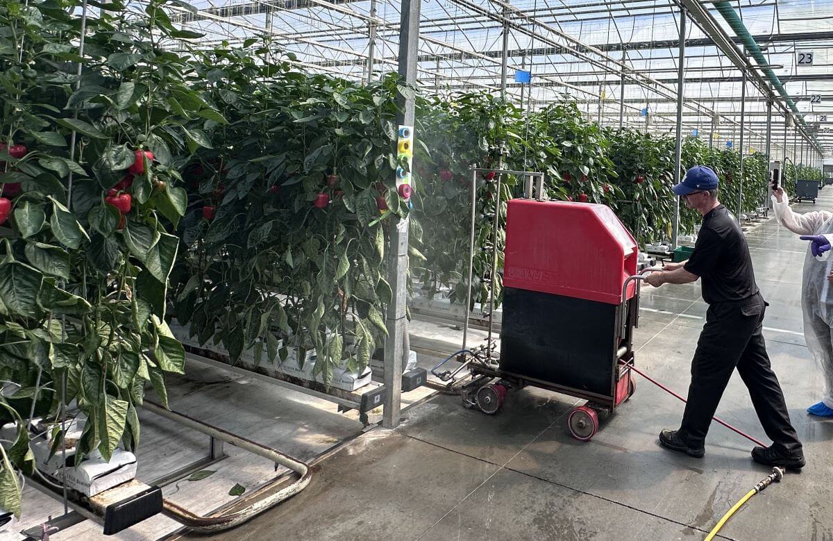
    Cedarline uses semi-automatic “robot trees” (Wanjet model S55). This sprayer has a vertical, 2 m high boom with nozzle bodies spaced every 25 cm. When the crop grows higher than the boom, an extension is added to bring it to 4 m. Flange wheels allow the sprayer to ride the hot water pipes between the rows like a train on rails at a rate of 60 m/min.

    The sprayer is manually placed in the row. Then it trundles along, spraying one side, until it reaches the end of the row. Then the vertical boom turns to spray the other side on the return trip, where it is retrieved and placed in the next row. The sprayer is fed from a portable tender unit via a 180 m auto-reeled hose at 200 psi. The question is, does this all work the way we assume?

    4. Calibrating the sprayer

    4a. Pressure

    We started with pressure. If pressure is the force that causes a specific volume of spray mix to exit the nozzles at a specific rate and produces a specific droplet size and spray geometry (e.g. a cone or a fan), then it’s very important to know that it’s accurate.

    Remove the gauge with a wrench (never turn it by the face) and test it against a known gauge. You can build a test apparatus very easily. Alternately if the gauge is showing wear, such as the needle not sitting on the zero pin, or it’s opaque, or leaking, maybe just replace it without testing.

    In our case, we discovered the gauge was off by 20%. Where the standard gauge read 150 psi, the working gauge read ~120 psi. Plus, the scale of the gauge was far too high. Best practice is to use a gauge rated to about double the operating pressure. This gives better resolution, and a quick glance shows if the needle is pointing straight up.

    I prefer a tender system like this over a central spray tank in a header house. In systems where there is a central tank and the sprayer hoses plug in at intervals, the degree of pressure-drop increases with distance from the source. If this is you, install a regulator on your sprayer and adjust it accordingly to hold the pressure constant. In this case, the distance the spray solution travels is always constant, so the pressure doesn’t change. Best practice in either case is to install a pressure gauge on the sprayer at the end (or top) of the boom so you can confirm the operating pressure is correct.

    4b. Sprayer speed

    We were told the sprayer was set to travel 60 m/minute, but is that true? Certain chemistries will deposit a slick coat on the hot water pipes and the flanged wheels can slip (especially as they wear). There was obvious damage to the rubber surface of two of the flanged wheels that might have affected travel speed. We should have checked, but we didn’t. Use a timer and confirm how long it takes for the sprayer to travel to the end of the row. Don’t include turn time. If it doesn’t match your expectation, then adjust the speed until you get what you want.

    4c. Boom and nozzles

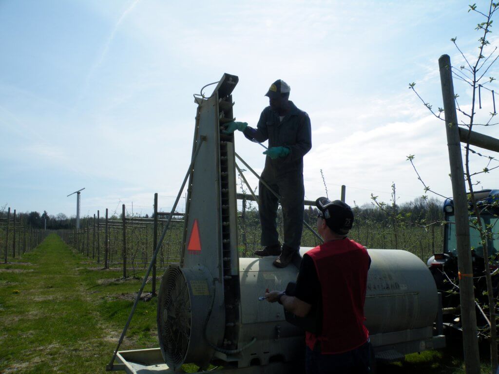
    Next, we explored the boom and the nozzles. The first thing we saw was that their alignment was wrong. Flat fans in ¼ turn nozzle caps will self-align on the lug to ensure each spray fan does not physically impact it’s neighbours. However, the nozzle bodies themselves can sometimes turn on the threaded boom, and they need to be realigned. We did that before removing a few tips for inspection.

    Each nozzle should be oriented 10-15 degrees off vertical and parallel to one another. Here, the top one is correct, but the lower nozzle has twisted and will leave a gap in the swath.

    I asked when the nozzles were last replaced and was told the sprayer arrived pre-nozzled with TeeJet visiflo 8002’s. They had never been inspected, other than when they plugged, and their rates had never been confirmed. Upon inspection we found some were physically damaged. This doesn’t mean the nozzle orifice was compromised, but it instilled doubt. You don’t always see obvious damage but know that the orifice is delicate and very precise. As it wears it gets larger (increasing flow), but more insidiously it also changes shape, altering the size of the spray droplets, which we’ve established are critical to our spray strategy.

    Best practice is to test nozzle outputs at a known pressure and replace them when they are 5% off the expected rate. Unless a nozzle gets physically damaged, replace them as a set so they wear as a set. When do they wear out? It depends on the nozzle material, the nature of what you’re spraying, the pressure and the amount of time they spend spraying. Here’s a link to an article that suggests several methods for testing nozzle output. Some are cheap and slow, others are fast and expensive, but they all work.

    If that’s not appealing, you can mark your tank and see how many rows you should be spraying versus how many you’re actually spraying. Ultimately, given the relatively minor expense of new tips versus the trouble of calibrating them annually, it’s often simpler to replace them at intervals. In this case it’s worth noting that the first 2 m of boom operates all season, while the extension is only added later, so they won’t all wear at the same time.

    We examined and then returned the original tips to the boom for the next part of the calibration. We noticed that the gaskets were stretched (crushed). This made it hard to put the nozzles back on, so they would also need replacing.

    We turned on the boom to ensure we had everything back in the right place, and noticed that when we stopped spraying, the boom slowly emptied through the lowest nozzles. That meant expensive products were left to dribble out every time the boom stopped spraying, which is wasteful. It hinted that the check valves, which are built into the nozzle bodies, were no longer working. Ideally, once the boom pressure drops below ~15 psi, each check valve diaphragm closes to prevent leaks. It also ensures the boom remains primed for the next pass. We advised that they should be replaced and to ensure the new bodies have the correct thread size. European sprayers rarely have the same thread as North American, so compatibility can sometimes be an issue.

    5. Evaluating spray coverage

    This is an iterative process, which means we test, evaluate, make a single corrective change, and repeat until we (hopefully) see what we want. Water sensitive paper (WSP) is a terrific tool for this process, but it has a few caveats:

    • It will react to any moisture, including a humid atmosphere, so handle it with gloves and don’t let it sit for too long.
    • The WSP surface is only a surrogate for a plant surface. Deposits tend to spread more on leaves, vegetables and fruits, but will always be smaller on the papers. So, only compare papers to other papers and infer that the actual crop coverage is better.
    • We really don’t know how much coverage is enough. It depends on pest pressure, product concentration and mode-of-action (e.g. contact or systemic). Generally, we like 10-15% of the surface covered with 85 deposits per cm2 on 80% of the targets. Sometimes it’s easier to imagine the pest on the paper – can it fit between the deposits?

    5a. TeeJet visiflo 8002 at 200 psi

    We started by establishing a baseline using their current nozzles and pressure. WSP was folded and clipped at the petiole so we could assess adaxial and abaxial surfaces. We placed them deep in the canopy so we were looking at the worst-case scenario, and then noted where we left them (use a ribbon or part of the greenhouse as a frame of reference or you’ll never find them again). We sprayed from one side, then examined them in situ, then sprayed from the other side so we could see the impact of cumulative coverage.

    After spraying from both sides, we saw excessive coverage on adaxial surfaces and marginal coverage on abaxial. For those that have tools to digitally scan and assess WSP, it worked out to 31% coverage and 225 deposits/cm2 on the adaxial side, and 2% and 16 deposits/cm2 on the abaxial. In fact, the adaxial side was so saturated (>25% coverage) that I don’t trust the deposit counts because of overlaps, but there it is. This is when we brought out the nozzle manufacturer’s catalogue (which you can also find online). We found their nozzle and looked up the flow table, which shows the relationship between pressure, output rate and droplet size.

    Those in greenhouses might find that their operating pressures are far higher than what is listed, but that’s no problem. Find the highest pressure and output rate listed in the table and call those “Known Output Rate” and “Known Pressure”. Now use the following calculation to extrapolate flow for a new pressure. It’s also worth knowing that higher pressure tends to mean a wider fan angle and finer spray droplets than are listed in the table:

    Unknown Output Rate (gpm) = Known Output Rate (gpm) × (square root of New Pressure (psi) ÷ square root of Known Pressure (psi))

    In this case, at 200 psi this nozzle should produce 0.45 gpm. If we go up one size from the yellow 02 tip to a larger blue 03 tip, we can produce a similar flow but using only 100 psi. This would put less strain on the system, but it would also make droplets larger, fewer and perhaps slower.

    5b. TeeJet visiflo 8003 at 100 psi

    We tried the 8003 at a lower pressure and saw that the deposits were obviously larger on the adaxial side, and not saturating, which is good. However, we saw insufficient deposit density on abaxial, which was a deal breaker.

    5c. TeeJet visiflo 8003 at 200 psi

    We left the blue 8003s and brought the pressure back up to 200 psi. Now the flow was increased to 0.67 gpm, and the droplets were finer, more plentiful and moved a lot faster. The adaxial surface went back to excessive coverage, but perhaps not as bad as with the 02s. The abaxial deposit density was improved, but still not sufficient. You can see the results of the three trials in the photo below. Go counter-clockwise from 1 (at bottom right) to 3 (at top).

    5d. TeeJet twinjet TJ6011003 at 200 psi

    It was time for a radical change. We replaced the single flat fan geometry with twinjet flat spray nozzles (TJ60-8003). We tried this because we’ve tried it in the past and it worked well. We retained a blue 03 rate, so we still produced 0.67 gpm at 200 psi. This nozzle also retained the 80° fan angle, but created two of them at 60° to one an other. This would change the spray trajectory, creating new opportunities for droplets to align with the targets. Perhaps most importantly, the twin fan nozzles would produce finer droplets than their single fan cousins, increasing the odds and perhaps and creating more “wind”.

    We saw far less differential between abaxial and adaxial surfaces, with deposit density greatly improved on both surfaces. While the adaxial face showed larger deposit diameters, they were close enough to require close inspection to determine which side was which; Coverage was more uniform, with no drenches and no misses. By the numbers we saw 34% and 523 deposits/cm2 on the adaxial side (again, hard to trust the counts here because of overlaps arising from >25% coverage) and 19.5% and 400 deposits/cm2 on the abaxial. We had a winner.

    It’s also worth noting that every time we sprayed, we observed the deposit on the fruit and leaves. None of the sprayer configurations caused run-off (e.g. drip points on the bottom of the fruit or tips of the leaves), which would suggest we were not using an excessive volume. Look closely at the following two pictures to see the beads of water and how they deposit. They look great.

    We also watched to see if spray passed through the row into the next alley. A little puff here and there is fine, because it meant the spray was reaching the far side of the row. However, spray that blows through the row excessively is wasted becuase it misses the target row and ends up on the greenhouse floor.

    Epilogue

    We were pleased with the result of half-a-day’s effort. We left our hosts with some homework:

    • Change the pressure gauge to one that is accurate and spans to 400 psi.
    • Replace all nozzles and gaskets and ensure they are properly oriented.
    • Time the sprayer to confirm travel speed is what they assumed.
    • Using the known speed, pressure, and boom output, do the math to account for the fact that they would now be spraying a higher volume than they were. This will change how much product they put in the tank.
    • Watch the crop closely to ensure these changes do not compromise crop protection.

    Everyone learned a lot from our day together. Cedarline said they would calibrate their other sprayers using this process. They are even going to try a set of yellow 02 TwinJets to see if they can achieve sufficient coverage at their current pressure, which would mean they can continue to mix product at the same concentration. Those are pretty small orifices, guys, so watch out for plugged tips and good luck!

    Hopefully this inspired you to look critically at your own operation and to follow these steps to calibrate and optimize your crop protection practices. Happy Spraying.

    Everyone here had helpful ideas during this process. Calibration is a team sport so make sure both your operators and managers are involved. Left to right: Ryan Bezaire – OMAFA Summer Student; Paul Brooks – IPM Specialist, Cedarline Greenhouses; Jason Deveau – Application Technology Specialist, OMAFA; Jimmy La Rosa – Operations Manager, Truly Green Farms / Cedarline Greenhouses; Richard Robbins – Technical Representative, Plant Products; Cara McCreary – Greenhouse Vegetable IPM Specialist, OMAFA
  • Adjusting Sprayer for Alternate Rows

    Adjusting Sprayer for Alternate Rows

    An “Alternate Row Middle (ARM)” traffic pattern is where the sprayer passes down every second row. The intent is to improve work rate by cutting the driving time in half. The operator hopes to provide suitable coverage on both the sprayer-facing half of the canopy, and that half of the canopy facing the next alley. In our experience, this depends on sprayer design, and only works in very small/young plantings (or only for the first few applications of the season). Even then, the side facing the sprayer tends to get saturated in an effort to ensure a threshold dose reaches the far side. We’ve already captured the pros and cons of ARM in this article, and (spoiler alert) unless you’re using a wrap-around style design, it’s generally not the best approach for protecting an orchard, bush, cane or vine crop.

    So why on Earth would we be testing it here?

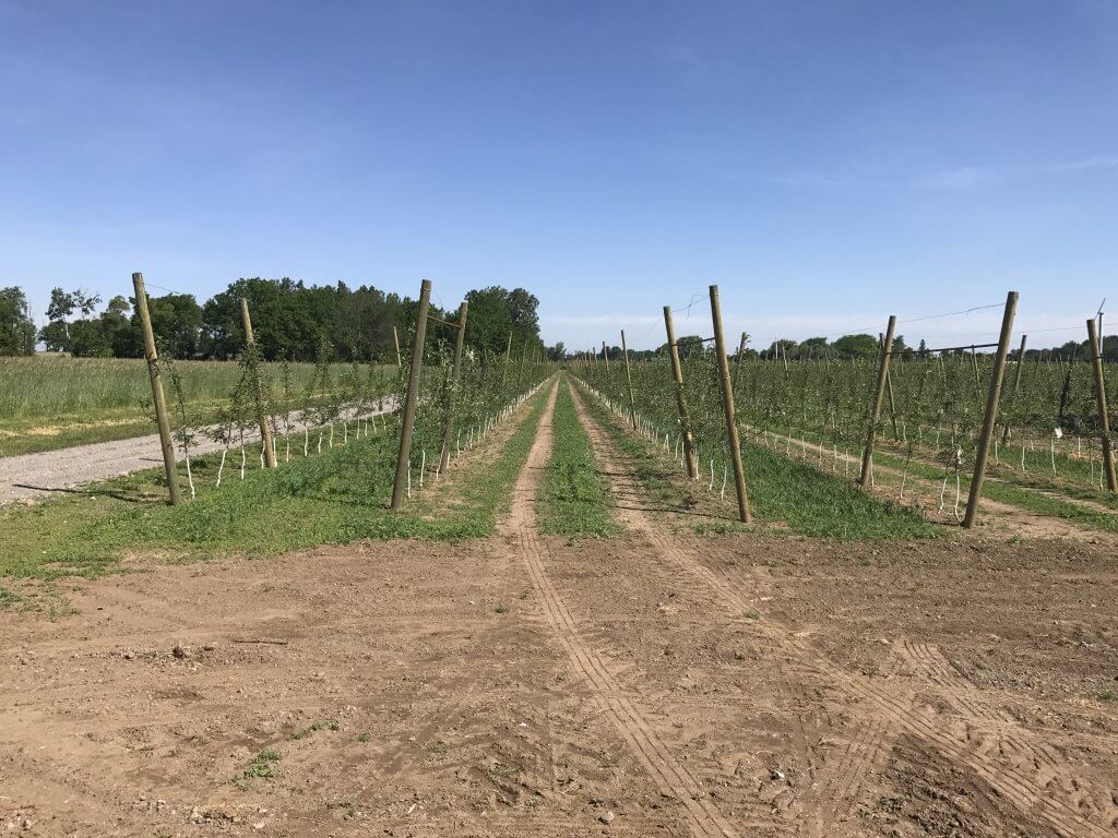
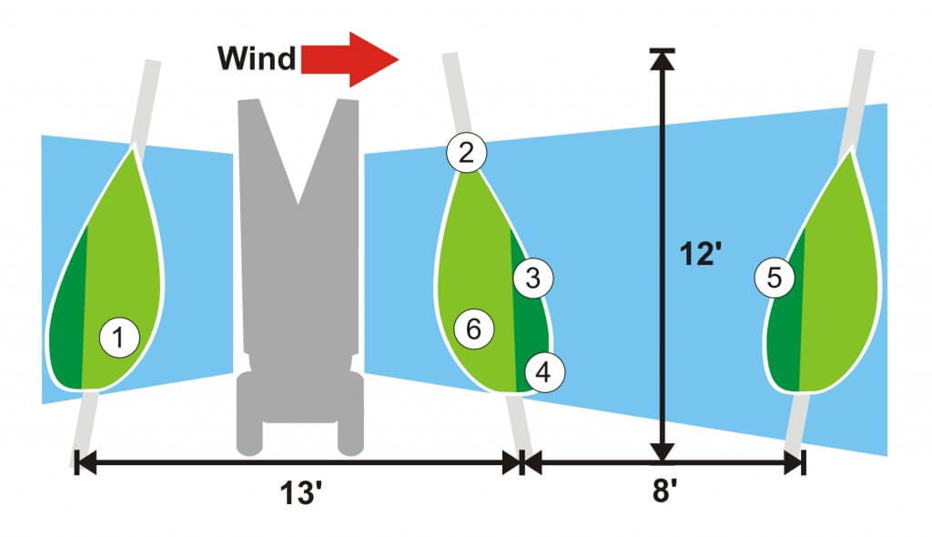
    We were contacted by an orchardist who planted a test block of Gala (est. spring, 2017) in an unusual way. He called it “V-Trellis Vertical Axis Cross”. Basically, he created an orchard architecture that only allowed equipment (e.g. platforms, sprayers) to pass down every second row. He figured it would save 35% of his labour costs. In the photo and illustration below, you can see the posts lean over the drivable alleys, creating a “V” shape.

    So, given that he couldn’t fit a sprayer down every row, we had no choice but to try to optimize sprayer settings for ARM applications. Note the six numbers in circles in the above illustration. They indicate where we would eventually place water-sensitive papers to diagnose spray coverage.

    Here are the settings the orchardist was using before we made any adjustments:

    • Turbomist sprayer with 11 foot high tower
    • Bottom-most nozzle was on and every second nozzle position skipped for a total of 5 nozzles active per side
    • Nozzles were TeeJet ceramic disc-core. Top to bottom: D3-DC45, D3-DC45, D3-DC45, D3-DC45, D3-DC25
    • 7 km/h (4.35 mph) travel speed per a speedometer app on a smartphone
    • Tractor engine speed was 2,150 rpm (PTO was ~ 540 rpm)
    • Fan set in low gear
    • Pressure was 190 psi
    • Ambient wind gusting to 8 km/h, temperature of 30°C, RH ~65%.

    And here is a video of what the sprayer was doing before we changed any settings. This is a single upwind pass, and as you can see, the spray blew through at least five downwind rows. Obviously, this was far too much air and spray volume.

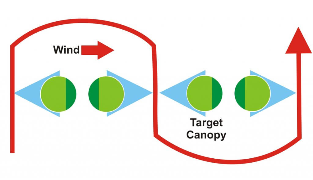
    When we diagnose coverage in an every-row situation, we drive the alleys on each side of the target row (i.e. two passes). But, when diagnosing ARM spraying, we want to account for every drop of cumulative coverage from spraying upwind rows. So, we have to do three passes, as shown in the illustration below. In this top-down diagram, the sprayer travels the red line.

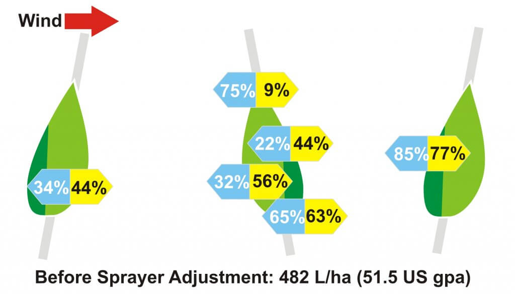
    In order to establish a baseline, we diagnosed coverage for the original settings using water-sensitive papers in the six positions indicated above. We folded them in half, so a sensitive side faced each alley. We sprayed water and later digitized the cards to determine the percent coverage on the papers. Remember, if 80% of the cards receive at least 10-15% surface coverage and a deposit density of 85 drops per cm2, it’s typically sufficient.

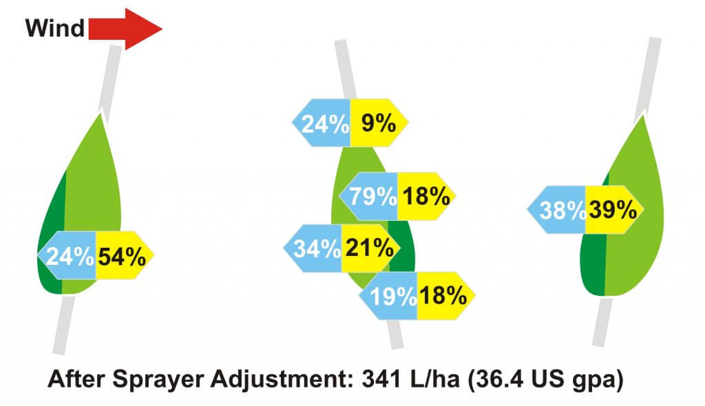
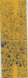
    Here are our results, with percent area-covered indicated in each position, as well as a representative scan of one of the papers. There’s no need to provide deposit density, which after about 30% surface coverage cannot be reliably determined.

    So, if the video doesn’t convince, then the papers certainly do: This was way too much air and spray mix.

    Next, we performed a series of air adjustments using ribbons (detailed here and here) which led us to reduce engine speed from 2,150 rpm to 1,300 using the Gear-Up, Throttle-Down method. Then we used the OrchardMax calculator to establish an ideal spray volume and guide us to which nozzle rates we should use:

    • Bottom-most nozzle was on and every second nozzle position skipped for a total of 5 nozzles active per side
    • Top nozzle was TeeJet AITX8002, followed by TeeJet TXR80015, TXR80036, TXR80015, TXR80015
    • 7 km/h (4.35 mph) travel speed per a speedometer app on a smartphone
    • Tractor engine speed was 1,300 rpm (PTO was ~ 300 rpm)
    • Fan set in low gear
    • Pressure was 100 psi
    • Ambient wind gusting to 4 km/h, temperature of 26.5°C, RH ~70%.

    The following video shows the coverage from a single pass (to be clear, no extra upwind pass). We eventually did three passes to capture the cumulative coverage, just like with the first sprayer settings. This video simply serves to show how in ARM applications, the sprayer-facing side always looks much better than the side facing away. Also note how much quieter the sprayer is, as well as the reduced blow-through.

    And here is the resultant, cumulative coverage from three passes. Once again, deposit density isn’t required as it exceeded our threshold in each position.

    In the end analysis, we saved the grower ~30% of their spray mix, greatly reduced noise and spray drift, and still achieved suitable coverage in the target canopy. So, does this mean ARM applications are redeemed? We refer you, kind reader, to our introduction where we said ARM can work in young plantings and early season applications.

    Note that the upwind side of the canopy received less coverage than the downwind side. As this new planting grows and fills, it’s going to be increasingly difficult to achieve sufficient coverage. Changes to the sprayer settings may be able to account for the imbalance, but they will also make the applications less efficient (i.e. more spray mix, more drift and coverage will still not be uniform). It remains to be seen if the spray inefficiency inherent to this orchard architecture is worth the estimated 35% savings in labour costs.

    It’s an economic decision. We’ll see.

  • Calibration – “The Fundamental Relationship”

    Calibration – “The Fundamental Relationship”

    The Fundamental Relationship, a concept by Professor D. Ken Giles (Emeritus), UC Davis Biological and Agricultural Engineering Department, is a way of talking about calibration without numbers and formulas. It is valuable for teaching concepts important to calibration. Since it is a relationship, it describes the variables needed and how they relate to each other.

    The Fundamental Relationship:

    Application Rate (gallons/acre) = Flow rate (gallons/minute) ÷ Land rate (acres/minute)

    We see here that land rate is inversely proportional to application rate. Thus, when land rate (either speed or swath width or both) are increased (and no other factors change), application rate is decreased. Likewise, flow rate is directly proportional to application rate. Thus, when flow rate is increased (and no other factors change), application rate is also increased. When flow rate is decreased (and no other factors change), application rate is also decreased.

    The Fundamental Relationship is also a good way to do the math of calibration because nothing needs to be memorized. As long as the units are checked, you can’t go wrong. The Fundamental Relationship works for any sprayer calibration, as long as the units are tracked correctly and the flow rate correlates to the land rate, i.e., the land rate used is the swath that the nozzles (flow rate) are covering.

    So, if the flow rate (GPM) used in the formula is for ½ of an airblast set up, the swath width in the land rate calculation would be ½ of the row width. If, for example, it is for a weed sprayer with 2 nozzles, the swath width would be the width the 2 nozzles are covering. Remember to think about this as what area is being covered by the spray:

    • Flow rate units are straight forward: gallons/minute.
    • Land rate can be a bit tricky because no one thinks in terms of acres covered per minute.
    • Land rate is tractor speed × swath width covered by the nozzles used to calculate flow rate.

    Land rate in the above needs to be calculated in the units “ac/min”. Since there are 43,560 ft2 in an acre, the easiest way to calculate is to use the swath width in feet, and the speed in ft/min. Multiplied, this then will give you land rate in ft2/min, which can then be converted to ac/min.

    Using MPH as Speed

    When you measure speed in the field, those who have a speedometer on their tractor will tell you their speed in MPH. To go from a land rate with speed as MPH to ac/min, the following unit conversion is used when multiplying the speed in MPH times the swath width in feet:

    1 mile/5,280 feet × 43,560 ft2/1 acre × 60 minutes/1 hour = 495
    Land rate (ac/min) = (Speed (mph) × swath width (ft)) ÷ 495

    Note: speed should always be measured and verified. Speedometers are notoriously incorrect!

    Calculating nozzle flow rate (GPM):

    You can also use the Fundamental Relationship to calculate the flow rate needed for a desired spray volume (application rate) when you have a set land rate (speed and swath width). This is necessary to help you choose your nozzles. Tractor speed is first determined by checking the coverage-using water sensitive paper or another coverage indicator like kaolin clay, and the fan (using ribbons in the canopy), to go as fast as safely possible while still getting adequate coverage. Swath width for any given field is set. What is left then is to calculate the GPM needed to achieve that application rate at that speed and swath width. This will allow you to select your nozzles based on individual nozzle GPM for a certain pressure.

    The Fundamental Relationship becomes:

    Flow rate (gallons/min) = Application rate (gallons/acre) × Land rate (acres/min)

    This is the flow rate for the ENTIRE sprayer (both sides, correlating to the swath width):

    GPM = GPA × Land rate

    OR if using MPH for speed:

    GPM = GPA × [(Miles/Hour × swath width (ft)) ÷ 495]

    To get the required GPM for one side of the sprayer, you multiply by ½:

    GPM (one side of sprayer) = GPA × [(Miles/Hour × swath width (ft)) ÷ 495] × 1/2

    GPM (one side of sprayer) = GPA × [(Miles/Hour × swath width (ft)) ÷ 495]

    I’ve seen some folks round up the 990 to 1,000, which makes the above formula easier to remember.

    Why I think the “495 formula” is bad for calibration

    In my experience of teaching calibration math, folks often want to fall back on the formula they have used instead of trying the Fundamental Relationship. The problem I have with the “495 or 990” formulae, is that with using ground speed in MPH, often the step of measuring speed, a critical step for optimizing spray coverage, is eliminated.

    Ground speed is assumed, the speedometer is assumed to be correct, and the entire step of measuring and setting speed is omitted-big mistake! Setting speed using flagging tape in the canopy and looking at the “Fan : Speed : Canopy” interaction is probably the most important step of calibration and optimizing coverage. So, if you must use the “495 formula”, please actually measure your ground speed!

    Measuring speed manually

    Typically, at least 100 feet are marked off to measure actual speed with a stopwatch. If you measure actual tractor travel time for a 100 foot length, you will likely find most common spraying speeds are timed in seconds. These can be converted to minutes, and then used in the formula for speed as ft/min which is then multiplied by the swath (or row) width in feet to obtain ft2/min, which can then be converted to ac/min.

    For example, at 3 MPH, you are travelling:

    3 mph × 5,280 ft/1 mile × 1 hour/60 minutes = 264 ft/min

    If swath width is 6 feet, the land rate (or area the nozzles are covering) is calculated as:

    264 ft/min × 6 ft = 1,584 ft2/min

    In acres covered per minute, we divide by 43,560 ft2/ac to obtain a land rate of 0.036 ac/min. To travel 100 feet at this speed, it takes 0.37 minutes or 22.7 seconds. So, it is not uncommon to time 100-foot tractor runs in 21-23 seconds (which is why you need a good stopwatch). These runs are best done on the type of terrain to be sprayed; and it’s always good to take several times and average.

    Remember that the speed is written as distance travelled/time. Sometimes when measuring speed, I’ve noticed that it will be written as time/distance travelled, which gives the wrong number. Track units!

  • How to Size a Nozzle for Pulse Width Modulation (PWM)

    How to Size a Nozzle for Pulse Width Modulation (PWM)

    PWM is gaining popularity, and there is an ever-increasing number of first-time users that need to make nozzle selections for their system. We’ve written about it here, here, and here.

    Recall the PWM replaces spray pressure with Duty Cycle (DC) of a pulsing solenoid as the primary means of controlling nozzle flow. The solenoid shuts off the flow to the nozzle intermittently, between 10 and 100 times per second depending on the system. The Duty Cycle is defined as the proportion of time that the solenoid is open, and for low-frequency systems, DC is more or less linearly related to flow rate.

    The first rule of PWM nozzle selection is to understand that under average travel speeds, we’d like to see the duty cycle of the system at between 60 and 80%. This means that the nozzle solenoid is open about 2/3 of the time. This value also describes the flow rate as a proportion of the full capacity that nozzle.

    The reason for this 2/3 duty cycle rule is to enable four key features of PWM:

    1. It’s ideal for turn compensation, allowing the outer nozzles to increase their flow 20 to 40%, and the inner nozzles to decrease flow about three-fold, in accordance with boom speed.
    2. It allows speed flexibility, providing some additional speed, but more importantly, reduced speeds should conditions require it, without a change in spray pressure.
    3. It compensates for pressure changes so that spray quality can be adjusted without requiring a speed change. Less pressure reduces nozzle flow, and increasing DC recoups accordingly.
    4. It allows for customized higher flows of certain nozzles, perhaps behind wheels, to address reduced deposition in their aerodynamic wake (available on some PWM systems).

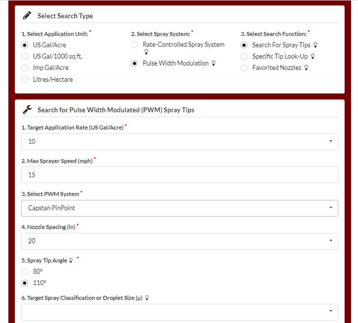
    The best tool for selecting the right nozzle size is Wilger’s Tip Wizard. This site asks for your desired average speed ( although it calls this “Max Sprayer Speed”), and reports the expected DC for a host of nozzle size solutions and pressures. It also reports maximum and minimum travel speeds and other useful information such as spray quality.

    Fig 1: The Tip Wizard is a useful tool for sizing nozzles on any PWM system. Sizing information applies to any nozzle. Spray quality information is for Wilger ComboJet nozzles only.

    Although intended for Wilger nozzles, the site’s sizing feature works for any nozzle brand. It asks the user which PWM system they have for the purpose of calculating the documented pressure drop across the solenoid.

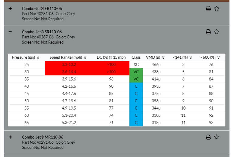
    Fig 2: Tip Wizard results for the Wilger SR11006 tip at 10 gpa and 15 mph. Look for a solution that provides 60 to 80% Duty Cycle (DC).

    If you don’t have access to the site, a basic calibration chart can still work with a simple trick. Recall that we use the top row to identify the desired water volume, and the table’s interior values are speeds, as described here.

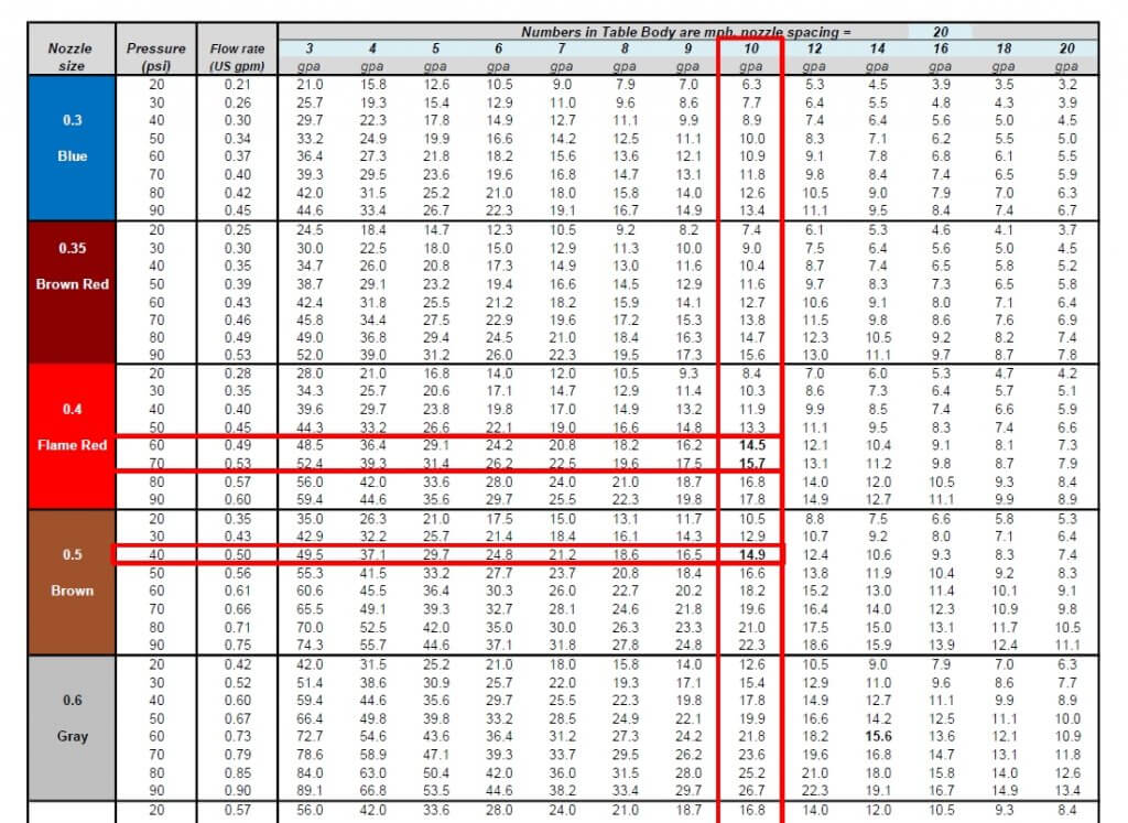
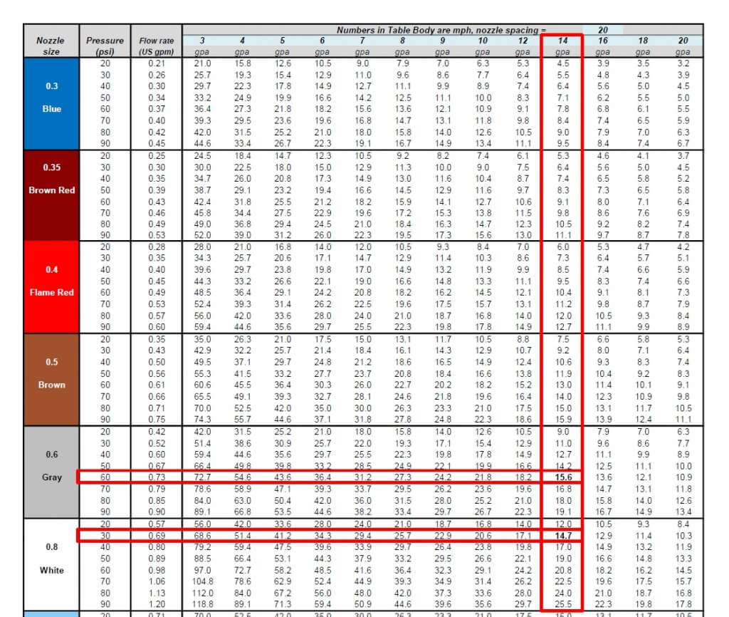
    Below are two solutions for someone wanting to apply 10 gpa at 15 mph without PWM. The correct choice depends on the required pressure to produce the needed spray quality.

    Fig 3: A conventional calibration chart, solving a 10 gpa application for 15 mph.

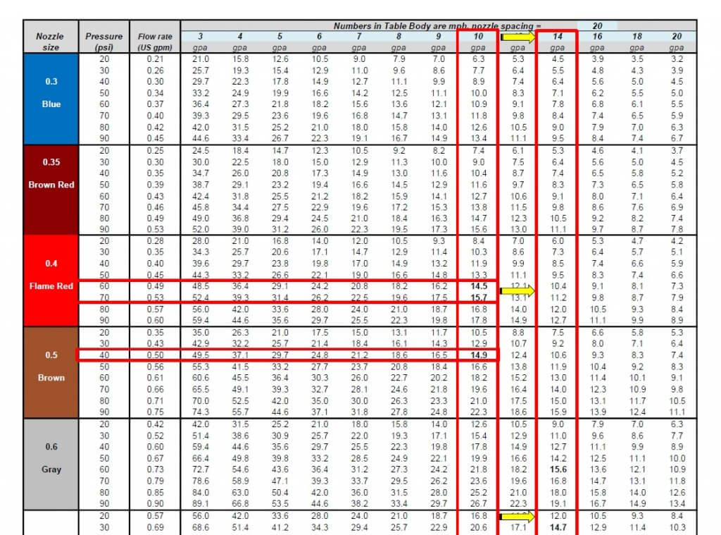
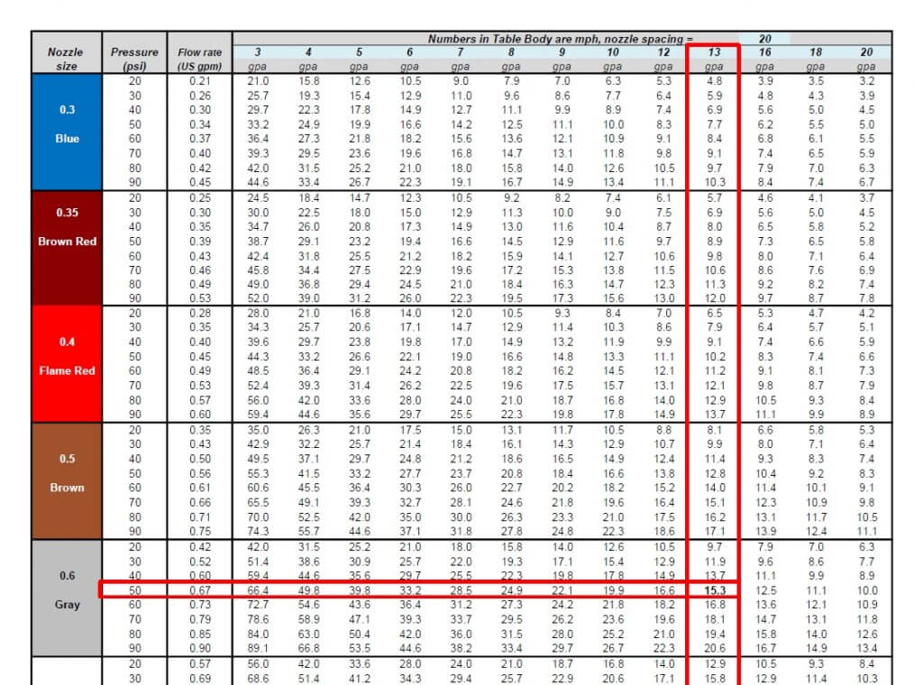
    If you want to apply the same 10 US gpa using PWM, simply solve for a larger volume that offers the right DC. For example, choosing 13 gpa will over-apply by 3 gpa, or 30%. The PWM system adjusts by running at 100-30=70% DC. If the chart doesn’t offer 13 gpa, go nearby, to 14 gpa, as we did below:

    Fig 4: By pretending to require 14 gpa instead of the actual 10 gpa, the conventional calibration chart is tricked into solving for a nozzle size that will work with PWM at 60% Duty Cycle.

    Now solve for the same target speed, 15 mph. The solution will run at 60% DC. Again, there is more than one choice, and that will depend on the spray pressure needed.

    Fig 5: Two possible solutions for achieving 10 gpa at 10 mph. An 06 nozzle at intermediate pressure or an 08 nozzle at low pressure.

    We’ve developed a template, in US or metric units, that can be customized for any water volume. Here is the same chart with 13 gpa added:

    Fig 6: A conventional calibration chart with the 13 mph speed added.

    The best solution for 10 gpa at 15 mph is the 06 size nozzle at 50 psi. This is not engraved in stone. One of the nice things about PWM is that it has inherent flexibility. Make the nozzle pressure a priority to get the correct spray quality. It really doesn’t matter whether the resulting DC is 65 or 80%, the system will still work well. Simply avoid extremes that take you below 50% or above 90%, they will limit the system’s capabilities.

    The worksheet can be downloaded below:

    It can handle any water volume or nozzle spacing by filling in the blue cells. Two additional worksheets in the file automate the process, simply enter the desired application volume, travel speed, and nozzle spacing (yellow cells), and the solution that offers the optimal duty cycle range will be highlighted in light green.

  • Airblast Nozzles – On or Off?

    Airblast Nozzles – On or Off?

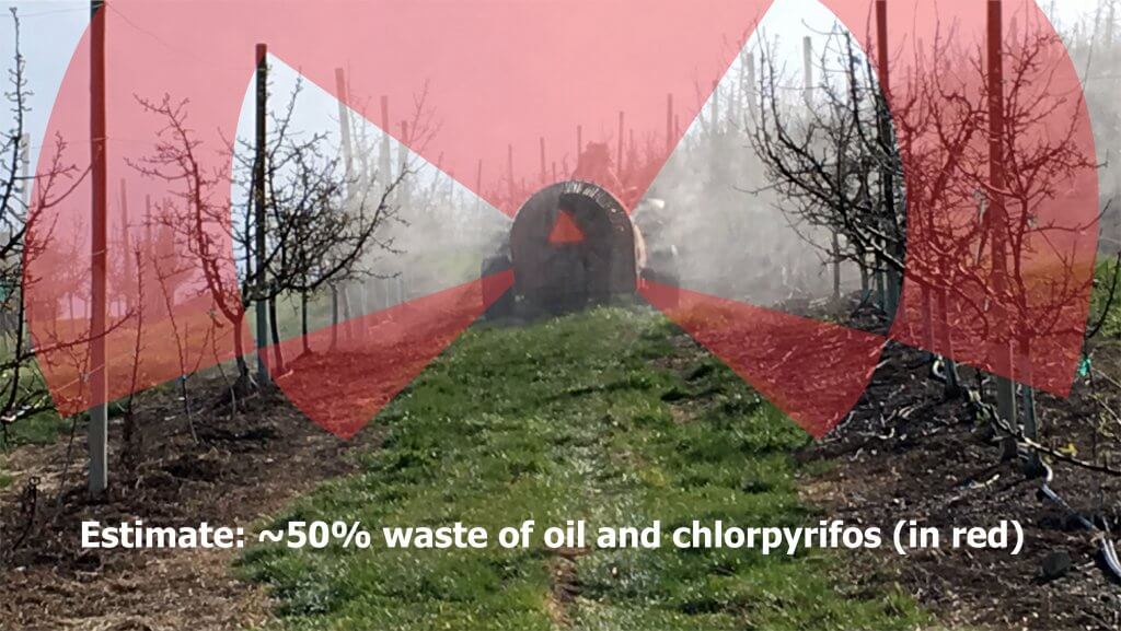
    Spray that is not directed at the target is wasted spray. Many pesticide labels specifically require the operator to restrict spray to the target canopy. Spray that escapes above the canopy is a significant source of off-target drift. Foliar applications that extend below the canopy are not efficacious and represent waste and lost productivity.

    A spring application or oil and chloropyfiros. Estimate of 50% waste (in red).

    Air carries spray droplets, so the first step in any adjustment should be to perform a ribbon test to ensure the air outlets are oriented correctly. This is achieved by adjusting deflectors (e.g. low profile axial), the air outlets on a tower, or the entire head on a wrap-around design with individual fan/nozzle combinations.

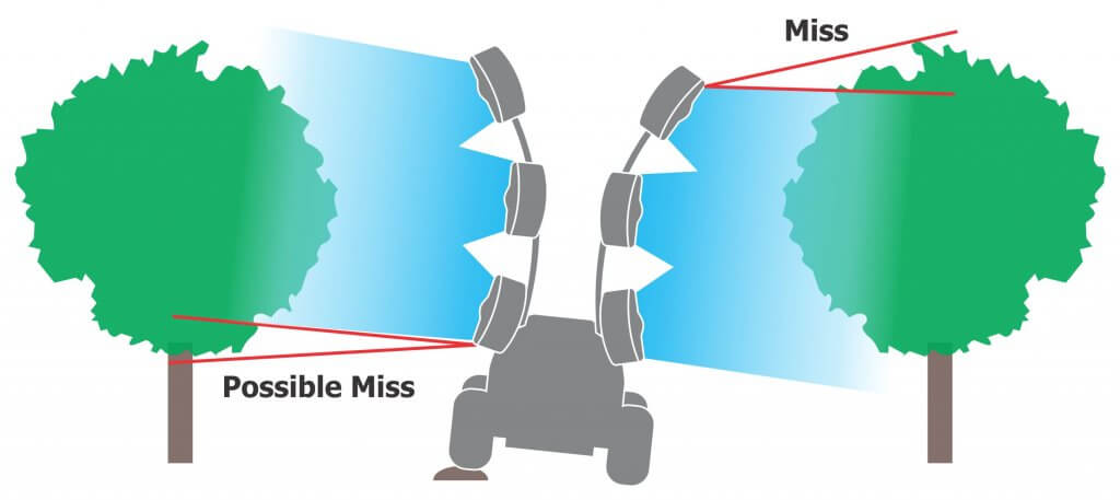
    Spray height should always exceed the canopy height by a small degree. This compensates for the increase in wind speed with elevation, the potential loss of spray height with faster travel speeds, and uneven alleys that cause the sprayer to rock, which changes the spray angle.

    Spray angles change as a sprayer rocks on uneven alleys. It is more important that spray is directed at the top of a canopy than at the bottom.

    It is less critical that spray align with the lower portion of the canopy. As air energy wanes, or as droplets begin to lose momentum, finer droplets will slowly fall, depositing on random surfaces. Coarser droplets will quickly fall towards the bottom of the canopy, settling primarily on upward-facing surfaces. This secondary deposition can also occur from the cumulative impact of blow-through from upwind rows.

    Once the air is aligned, park the sprayer in an alley. Stand behind the sprayer and extrapolate a direct line from each nozzle to target canopy. Nozzles that point at the canopy should be left on. Nozzles that point above or below can be blocked, or turned off via valves or rotating roll-overs. Some roll-over nozzle bodies can be swiveled up or down 15 degrees to fine tune the spray angle. An alternative would be to permanently rotate the nozzle body fitting in the boom line. When aiming nozzles using a roll-over nozzle body, be careful not to swivel them too far or the valve will partially close and compromise the spray pattern.

    Use a ladder when adjusting nozzles on a tower sprayer. Some sprayer chassis and tanks are designed to accept a climber, but even so they can be slippery. Please be careful.

    When extrapolating, remember that the centre of a nozzle only indicates the centre of the spray pattern. Cone and fan angles can span 60 to 110 degrees, depending on the influence of air. Therefore, even though the centre of the lower-most nozzle intersects the bottom of the target canopy, you may still be able to turn it off because the nozzle above has that portion covered.

    Adjust spray distribution across the boom at the beginning and roughly mid-way through the spray season to ensure the sprayer will uniformly cover the target with the optimal volume. These adjustments should account for both canopy growth and fruit set.

    For example, as the season progresses in an orchard, fruit may cause limbs to hang lower and warrant a new spray distribution. Turning on the bottom nozzle position will help, but it doesn’t account any increase in density throughout the canopy. You may need more volume distributed across the entire boom. Another example: as grape bunches begin to close, sprayer operators may direct fungicides exclusively at the fruit zone and not the entire canopy.

    Remember to always check coverage using water sensitive paper. It’s not worth saving a bit of spray if you’re missing a bit of your target.