Category: Boom Sprayers

Main category for sprayers with horizontal booms

  • Evaluating Electrostatic Spraying in Carrot

    Evaluating Electrostatic Spraying in Carrot

    This research was performed with Dennis Van Dyk, OMAFA Vegetable Crop Specialist.

    In 2018, MS Gregson introduced a line of electrostatic sprayers (the Ecostatik) in Canada. While electrostatic technology has been used in agriculture since the 1980’s, this is the first time ground rigs have been so readily available to Ontario (possibly Canadian) growers.

    The 3-point hitch Ecostatik can be configured for vertical booms or for banded/broadcast applications. The largest version has a 150 gallon tank, 10 gallon rinse tank and 72 nozzles on 7.5″ centres on a 60 foot boom. That model requires a 75 HP tractor, but 100 HP is preferred. The manufacturer claims the Ecostatik uses 50% less spray mix, gives superior underleaf coverage, and loses less spray to the soil compared to conventional methods.

    Ecostatik 3-point hitch electrostatic sprayer. 14′ boom model pictured.

    Objective

    In the summer of 2018 we evaluated and compared the electrostatic sprayer to conventional application methods at the University of Guelph’s Holland Marsh Research Station. Our goal was to assess spray coverage and physical drift in a vegetable crop.

    Treatments

    • Treatment 1: Conventional Hollow Cone (HC) at 53.5 gpa (500 L/ha).
    • Treatment 2: Conventional Air Induction (AI) flat fan tip at 50 gpa (468 L/ha).
    • Treatment 3: Ecostatik at 11.8 gpa (110 L/ha): electric charge on.
    • Treatment 4: Ecostatik at 11.8 gpa (110 L/ha): electric charge off.

    Sprayer set-ups

    Conventional Sprayer

    • 11.5 ft (3.5 m) boom with 20” (50 cm) nozzle spacing set 18” (45 cm) from nozzle to top of crop.
    • Treatment 1: D3-DC25 HC @ 140 psi and 3 km/h. SC-1 SpotOn calibration vessel (SC-1) gave an average flow of 1.36 L/min (0.36 gpm). Very Fine spray quality.
    • Treatment 2: AI11003 AI @ 80 psi and 4 km/h. At 50 psi, SC-1 gave an average flow of 1.21 L/min (0.32 gpm). Very Coarse spray quality.

    Ecostatik Sprayer

    • 15 ft (~4.5 m) boom with 7.5” (19 cm) nozzle spacing set 18” (45 cm) from nozzle to top of crop.
    • With tractor set to 2,100 rpms, avg. air speed was measured using a Kestrel wind meter. The turbulent nature of the air precluded testing with a Pitot meter. At 5″ from the nozzle: 71.5 mph (32 m/s). At 10″: 37.5 mph (16.6 m/s). At 18″ (target distance): 21 mph (9.4 m/s).
    • The MaxCharge nozzles contained TeeJet CP4916-16 flow regulator orifice plates. At 25 psi they should have emitted 0.020 gpm. However, the SC-1 indicated a consistent 0.034 gpm from multiple nozzles. We postulate that the air assist created a low pressure environment that increased flow. Extremely Fine spray quality.
    • Treatment 3: Electric charge of -16 µA (tested using a voltmeter set to 200 µA) and speed of 3.7 km/h.
    • Treatment 4: Electric charge off and speed of 3.7 km/h.
    The Ecostatik boom
    Testing electrostatic charge with a voltmeter. Hair standing on end was a fun extra.

    Experimental Design

    Fluorimetry

    We used the fluorescent dye Rhodamine WT as a coverage indicator. This allowed us to take tissue samples to evaluate deposition, rather than rely on analogs like water sensitive paper. Further, the dye is detectable in parts per billion concentrations, making it sensitive enough for detection in drift studies.

    • The conventional sprayer received 40 gallons (151.5L) of water dosed with 303.5 mL dye (i.e. 2 mL / L).
    • The electrostatic sprayer 20 gallons (75.75 L) of water dosed with 151.5 mL dye (i.e. 2 mL / L).
    • A sample of the tank mix was collected from the nozzle prior to each application. It was later used to calibrate the fluorimeter for samples taken during that application.
    • Tissue samples were removed and dried to establish their dry weight.
    Rhodamine WT pooling on carrot (and weeds) as boom charged prior to application.

    Spray Coverage

    We chose to spray carrot on 20″ (50 cm) spacing on August 30, when the crop canopy was densest and represented the most challenging target. Our targets were leaflets located about mid canopy depth, and 1″ lengths of stem just above the crown. A diagram illustrating the experimental design appears later in the article.

    Fluorimetry lab station. Inset: A typical length of stem and a leaflet with a Sharpie for scale.
    Drawing a tank sample prior to application. Carrot canopy was mature and very dense.
    • 12 m blocks were randomly flagged for each treatment. There were 3 blocks per treatment. 4 treatments * 3 replications = 12 blocks.
    • Temperature, windspeed, humidity and time were recorded prior to each application.
    • Three plants were randomly sampled from each block. These sub samples were averaged to get a single data point. 3 replicated blocks x 4 treatments x 6 subsamples = 72 tissue samples (36 leaflets and 36 stems).
    • Samples were collected 60 seconds after spraying ended, placed in sample tubes pre-filled with 40 mL of water and immediately placed in the dark.

    Drift

    We also performed an analysis of physical drift for each treatment.

    • 4″ lengths of pipecleaner mounted vertically ~12″ above the crop canopy as drift collectors.
    • They were placed in a straight line from the middle of the boom at 1 m, 2 m, 4 m, 8 m and 16 m downwind.
    • Samples were collected 60 seconds after spraying ended, placed in sample tubes pre-filled with 40 mL of water and immediately placed in the dark.
    Spray coverage spray drift trial block design.

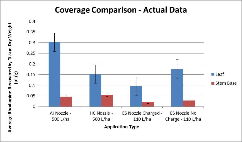
    The following graph shows the coverage observed in µL rhodamine per dry weight of tissue sampled. Bars represent standard error. Each treatment represents three passes (n=3) where each pass included three sub-samples averaged to offset the high variability inherit to spraying. While statistical analysis did not prove significant, there were strong trends. The AI nozzle deposited more dye on the leaves, while the HC and both electrostatic applications were par. Stem coverage achieved in conventional applications was approximately double that of the electrostatic. However, note that the electrostatic system only applied 1/5 of the volume sprayed conventionally.

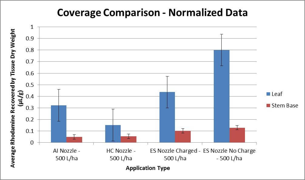
    When the data is normalized to depict a 500 L/ha application for all treatments, a different story emerges (see below). Now foliar coverage is 25-100% better for electrostatic applications than conventional. Stem coverage is twice that of conventional. Unexpectedly, the uncharged electrostatic treatment outperformed the charged treatment on the leaves. This might be the result of variability in the application, or the result of coronal discharge which can occur when pointy leaves repel charged droplets. This suspicion might be supported by the similar coverage achieved on the stems in both Treatment 3 and 4. You can read more about the Corona Discharge Effect in this article.

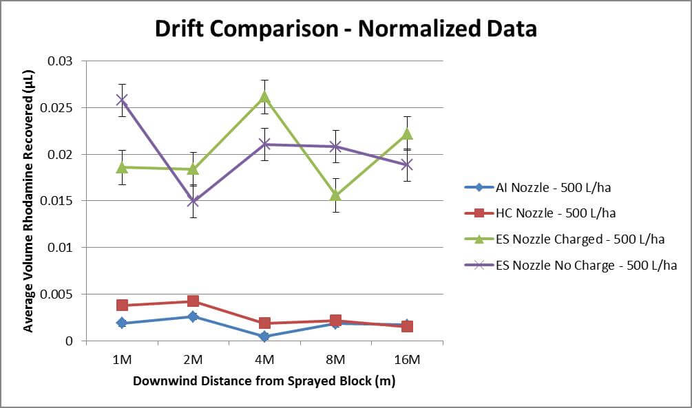
    Regarding drift, we will focus on the normalized data (where all treatments are adjusted to 500 L/ha). An analysis of variance indicated with 95% confidence that the electrostatic treatments drifted significantly more than conventional (approximately 5x more rhodamine detected). Particle drift follows an inverse square rule, where levels decline with distance, but the decline is only minor in all treatments. This may be a function of weather conditions, coupled with the limited distance investigated.

    Winds averaged 6.5 km/h gusting up to 10 km/h at boom height. Temperatures were between 15-17°C and relative humidity at ~70%. These conditions are conducive to drift as droplets are less likely to evaporate and in the case of Very Fine droplets, travel great distances. Many drift studies extend to 300 m from the point of application, whereas we were unable to monitor beyond 16 m. The downward trend would likely have been observed were we able to sample further downwind.

    Observations

    Our data supports the manufacturer’s claim that the electrostatic sprayer has the potential to match the coverage from a conventional application while using 50% less water and pesticide. It is unclear whether the electrostatic charge plays a role in this coverage, or if it is the result of the Very Fine spray quality and air assist (which have been demonstrated to improve canopy penetration). Further, it is unclear whether the charge may actually have been detrimental in the carrot crop. Claims of improved coverage uniformity were not explored in this study, but observations of water-sensitive paper in soybean (see image below) did indicate consistent under-leaf coverage, even at 50% application volume.

    The five-fold increase in drift potential is a significant barrier for this technology. The spray cloud is comprised of like-charged particles that expand in three dimensions, which improves coverage uniformity and penetration into the canopy, but also causes droplets to expand up and out of the canopy. Air assist is used to propel them downward, but the turbulent 9.4 m/s windspeed seemed excessive, even for a dense carrot crop.

    It is possible that focussing and reducing that airspeed may also reduce drift without compromising coverage. Presently, the air shear design of the Ecostatik’s MaxCharge nozzles prevent the operator from reducing the air speed without compromising spray quality. And, even if air speed could be reduced, the spray quality must remain Very Fine to achieve an optimal mass-to-charge ratio, and will therefore always carry an inherently high drift potential.

    Thanks to Kevin Van der Kooi for spraying, and Laura Riches, Tamika Bishop, Terisa Set, Christine Dervaric, Claire Penstone and Aki Shimizu for sample collection. Special thanks to Cora Loucks for assistance with statistical analysis and Martin Brunelle of MS Gregson for providing the Ecostatik for evaluation.

  • Air-Assist Improves Coverage in Field Corn

    Air-Assist Improves Coverage in Field Corn

    Why aren’t there more air-assist boom sprayers in Canada? I can understand why field croppers might hesitate to pay for the feature because it’s only been in recent years that fungicide applications have become a regular part of their annual spray program. But, high-value horticultural muck crops like onion and carrot, or field vegetables like tomato and peppers have been a great fit for many years.

    One operation near Dresden, Ontario was thinking the same way when they bought a used 2010 Miller Condor with a Spray-Air boom from Indiana. In the past, they employed a trailed Hardi sprayer applying 40 gpa using Turbo TeeJets alternating front-to-back in their field tomato and onion crops. They felt they could achieve better coverage with the air assist feature.

    On June 19 the onion and tomato canopies were still too sparse to be a good testing ground (and the ground was very wet). So, we decided to run coverage trials in a stand of 3 foot high corn on 30 inch centres.

    The Spray Air boom features a series of air shear nozzles on 10 inch centres. A liquid feed line meters spray mix to the orifice, where high-volume air is directed at the flow via two Cross-Flow jets. This shreds the liquid into spray and shapes a 60 inch flat fan pattern. The operator can select from a range of air speed/volume settings that affect spray quality (lower air means Coarser and fewer droplets and a smaller fan angle).

    This particular boom also carried a set of hydraulic nozzles, so the operator could elect to turn off the Spray Air feature and employ a conventional application. This would be appropriate if applying a herbicide using air induction nozzles. In this case, the sprayer was equipped with TeeJet FullJet cones.

    The first thing we noticed was that the air was not distributed evenly across the boom. We inspected the baffles that join each boom section, but found no problem.

    We then suspected the Spray Air combination nozzles might be occluded with debris (it did come all the way from Indiana). This turned out to be the case, so we popped them out and cleared the Cross Flow jets of any obstructions.

    We then measured the air speed produced by the boom. A Pitot meter proved to be too finicky to get a consistent reading, so we used a Kestrel wind meter held 12 inches from the nozzle. The operator moved between the six air settings in the cab, producing the following air speeds. Note that these speeds were much slower than the 100+ mph (160+ km/h) speeds noted in the Miller brochure. The owner has since told me that they found a number of air leaks in the boom that they have been diligently repairing, and as a result he’s operating at a lower air setting.

    Air SettingApproximate Airspeed at 12”
    14 mph (6.5 km/h)
    26.5 mph (10.5 km/h)
    38.5 mph (13.5 km/h)
    412.5 mph (20 km/h)
    515.5 mph (25 km/h)
    617.5 mph (28 km/h)

    We used water-sensitive paper wrapped around dowels to illustrate potential spray coverage.

    They were placed perpendicular to the spray at three depths in the corn canopy: High, Middle and Bottom. This provided an indication of panoramic coverage and represents a very difficult-to-wet target. In the last two trials, we also added a horizontal target at the Middle (not shown) and Bottom position to illustrate overall canopy penetration, and two at the High condition, angled at 45º into the sprayer’s path and 45º away from the sprayer’s path. These gave an indication of the highest potential coverage available to the canopy. Papers were later unfurled and digitally scanned. The papers were analyzed using DepositScan to determine the total percent coverage, and the droplet density.

    Trials took place between 8:30 and 11:00. Temperature slowly climbed from 20ºC to 23ºC (~ 70ºF). Relative humidity dropped from 69% to 60%. With the exception of Trial 1, we sprayed in a tail wind of 7.5 mph (12 km/h) gusting up to 10 mph (16 km/h). Travel speed was 7 mph (11 km/h).

    In the first five trials we made single, progressive adjustments to the spray settings that we assumed would improve coverage. Finally, we compared what we felt were optimal settings with the Spray Air (Trial 5) to optimal settings for the conventional hydraulic nozzles (Trial 6). Details are as follows:

    TrialAir settingSpray Volume (gpa)Boom Height (inches)
    121420
    23.51420
    361420
    46146
    56206
    6No Air – Fullcones206

    You can watch the passes in the following video. Note the boom height and the trailing spray.

    The following two graphs show the coverage obtained in the High, Middle and Bottom positions for all six trials. The first graph is percent coverage, and the second is droplet density.

    In trial 1 the air was insufficient to properly atomize the spray mix (as seen in the video) and this is evident in both graphs. By increasing the air in trials 2 and 3, we see that coverage increases in the High and Middle positions, but declines a little in the Bottom position. When we lower the boom closer to the canopy in Trial 4, we see increased coverage again in the High and Bottom positions, but lose ground in the Middle. We then increase our water volume for exceptional gains in the Middle and Bottom position, but at the expense of the High. Throughout these changes, overall coverage trended up. Finally, when we turn off the Spray Air system, and switch to the Fullcones, which were set to spray the same volume via the rate controller, there is a drastic reduction in coverage in all positions.

    Let’s look at the additional papers placed for Trials 5 and 6 in the following graphs.

    Even when papers were oriented to intercept the spray as much as possible, The Spray Air system provided superior coverage compared to the hydraulic nozzle.

    This leads us to conclude that there is an advantage to air assist in overall coverage and canopy penetration. Further, it demonstrates that such a system requires careful calibration to ensure it is being used optimally. Water volume, air settings and travel speed should all be reconsidered when the environmental conditions change (e.g. temperature and wind) and when spraying different crops, at different stages of growth.

    Two weeks after this trial, the corn grew too high for the Miller boom, but the grower moved into his onion and tomato and was very pleased with the overall coverage the Spray Air was providing. He’d also replaced the fullcones with 110 degree AI flat fans for herbicide spraying.

    I’d like to see more air-assist booms in Canada.

  • What is Delta T and why is it important for spraying?

    What is Delta T and why is it important for spraying?

    Click here to listen to Audio Article

    Humidity is important in spraying. With the average tank of pesticide being 90 to 99.5% water, evaporation plays an important role in both droplet size and active ingredient concentration. Low humidity causes droplets to evaporate faster, potentially increasing drift and reducing uptake. But relative humidity (RH) isn’t the best way to measure this effect because the same RH at two different temperatures results in two different water evaporation rates.

    Instead, we present Delta T, also known as “wet bulb depression”. Delta T is an atmospheric moisture parameter whose use in spraying has made its way to North America from Australian operations. It is defined as the dry bulb temperature minus the wet bulb temperature, and provides a better indication of water evaporation rate than RH. Higher Delta T means faster water evaporation.

    The recommendations from Australia are to avoid spraying when the Delta T is either too high or too low, with a range of two to eight being described as ideal.

    Figure 1: Delta T chart used in Australia (Source: Australian Gov’t Dept of Meteorology)

    Delta T is being reported on an increasing number of weather stations, and it’s time we took a closer look at what it means.

    Measuring Relative Humidity

    In the early days of weather reporting, relative humidity was calculated from psychrometric charts. All one needed was a hygrometer, usually a sling psychrometer. A sling psychrometer is two identical thermometers side by side whose bulbs could be slung in a circle, exposing them to moving air. One bulb was covered in a cotton wick moistened with distilled water, the other was left exposed and dry.

    Figure 2: Sling psychrometer (Source: ScienceStruck.com)

    As the bulbs met moving air, water evaporated from the cotton wick and that reduced the temperature of that thermometer. The dryer the air, the greater the evaporation rate and therefore the greater the temperature drop. The dry thermometer was unaffected by this movement.

    On measuring the wet and dry bulb temperature, one consulted a psychrometric chart. This chart converted the two temperatures to total water content in the air, compared it to total water-holding capacity, and expressed it as Relative Humidity. Psychrometric charts are useful for many other air parameters such as dew point, vapour pressure, or enthalpy. (Pause briefly to give thanks that we don’t need to know what enthalpy is.)

    Figure 3: Psychrometric Chart (Source: Carrier Corporation)

    Turns out that RH is a poor measure of water evaporation rate. An RH of 24% at 20 C has exactly the same evaporation rate as an RH of 44% at 35 C. That’s why Delta T is the preferred measurement: it’s linearly related to evaporation.

    Note: Modern electronic weather stations don’t need two thermometers to measure air moisture content, and use polymers whose capacitance or resistance changes with atmospheric moisture. Add an internal look-up table, and we have all the information we need.

    Pros and Cons of Water Evaporation

    It’s important to note that our Australian colleagues caution against spraying when water evaporation rate is both too high and too low.

    Too High:

    • Water evaporates rapidly, reducing droplet size and pre-disposing the smaller droplets to drift;
    • Deposited droplets dry quickly, reducing pesticide uptake which is more effective from a wet deposit.

    Too Low:

    • Water doesn’t evaporate, maintaining the smaller droplets in a liquid state. These small droplets are already drift prone, but are now more potent because of more effective uptake. Overnight conditions that are inverted are usually humid, adding to harm potential from the inversion.

    Delta T in North America

    The addition of this parameter to our spraying weather lexicon has been useful. But it’s important to understand the context in which it was developed to properly judge its suitability.

    Aussies started talking about Delta T because the use of finer sprays under the hot dry conditions found during their summer sprays resulted in significant evaporative losses, significantly greater drift potential, and potential reduction of product performance. The guidelines to avoid spraying when Delta T exceeds eight or ten originate there.

    A few changes have happened since these guidelines were developed. Over the past ten to 20 years, we’ve observed greater use of low-drift sprays, with the coarser sprays’ larger droplets resisting fast evaporation. In the past five to ten years, water volumes have increased due to our heavier reliance on fungicides, desiccants, and contact modes of action. Both of these developments have helped reduce the impact of a dry atmosphere. We simply can’t say if a Delta T of 10 is too high with these new application methods.

    Looking at it another way, if Delta T values are very high, increasing water volume and droplet size will mitigate that to some degree, as the Aussies state in their extension materials (linked earlier).

    Formulation

    Pesticide formulation can also play a role in evaporation. Once the water is gone, oily formulations may still have good uptake because the oily active ingredient stays dissolved in the oily solvents. This is both good and bad, helping on-target efficacy but also increasing the risk of more potent drift. Solutions, on the other hand, are more likely to leave their actives stranded on leaves as crystals once the water is gone.

    Bottom Line

    Delta T is definitely useful information when spraying. It will typically rise and fall with air temperature as the day proceeds, and it is wise to consider suspending operations when values are critical. Take note of the Delta T when spraying the same product throughout these hot days and learn from the experience. Remember, the atmosphere affects not just sprays but also plants and insects, and due to this complexity we may not be able to attribute success or failure to just one measurement.

  • Biobeds for Pesticide Waste Disposal

    Biobeds for Pesticide Waste Disposal

    One of the most challenging aspects of a spray operation is the disposal of leftovers or rinsate containing pesticides. Let’s be honest, too much of it is drained onto the ground in a corner of the yard or the field. Nobody’s happy about that, nobody’s proud of it, but what are the alternatives?

    Waste disposal is a skeleton in the closet of the pesticide industry. One of the problems is the time-consuming nature of sprayer cleaning, and the lack of clear guidelines on product labels that pass the buck.  Too often, the applicator is asked to “act in accordance with provincial or state guidelines”, which is essentially a dead end.

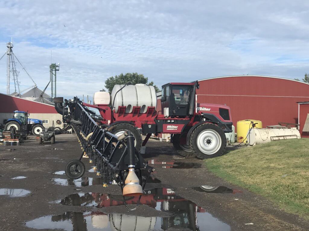
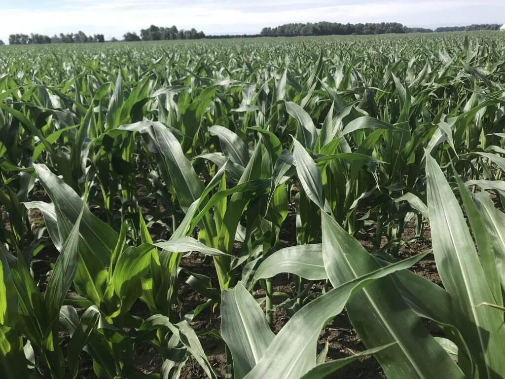
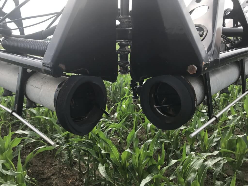
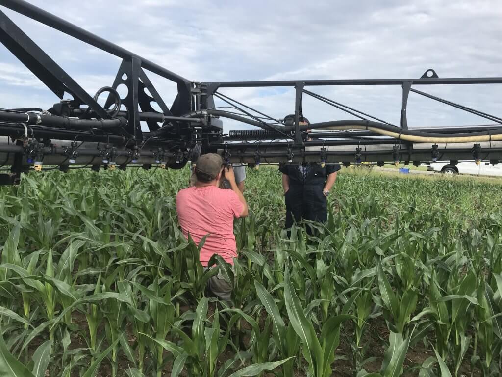
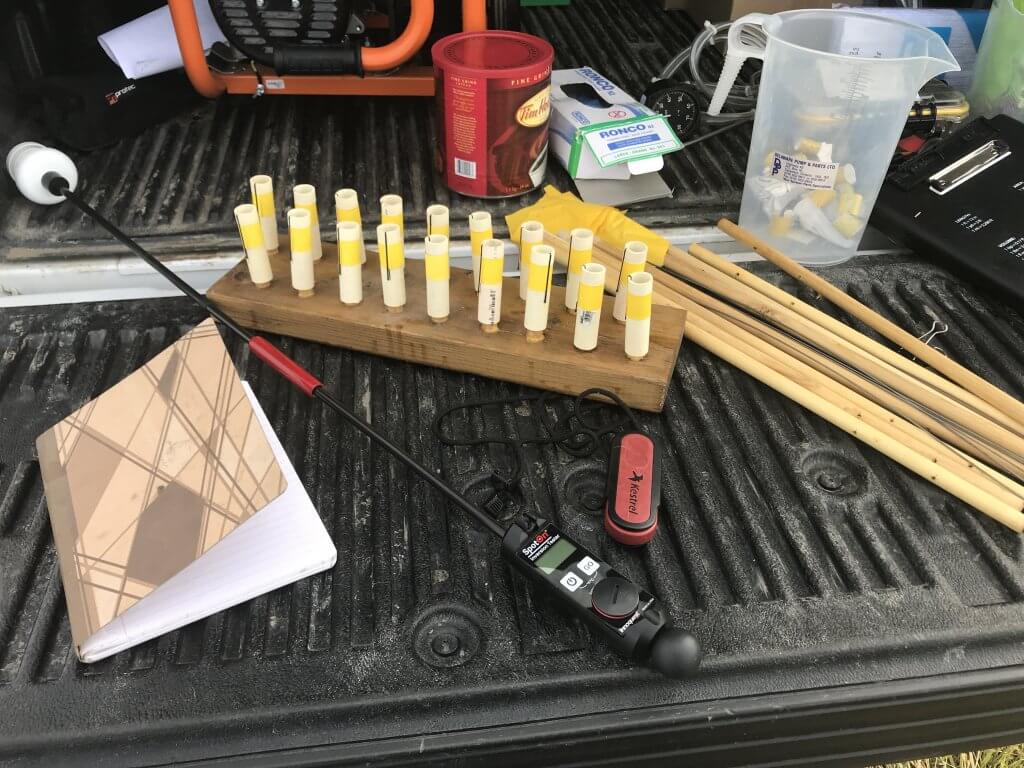
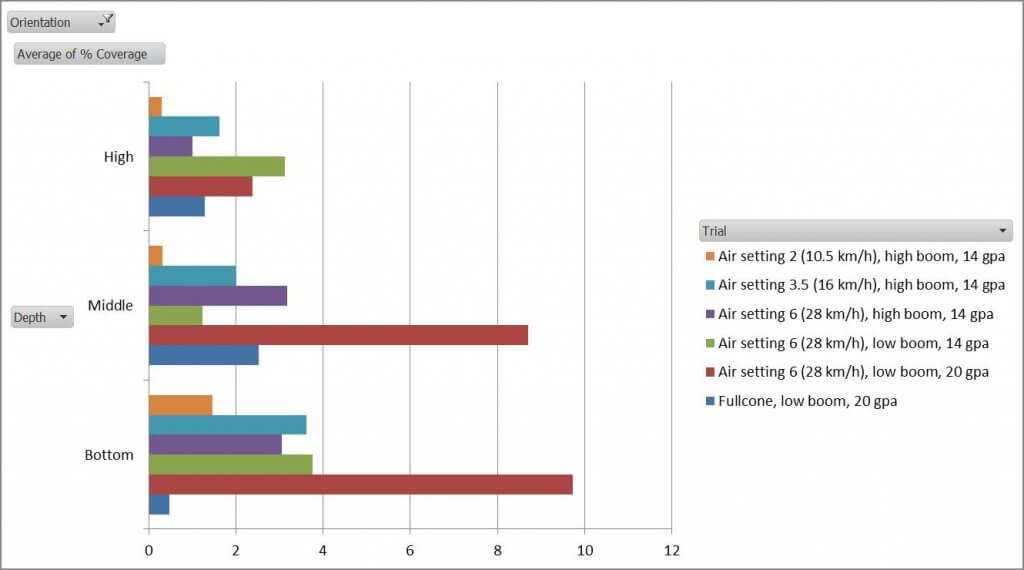
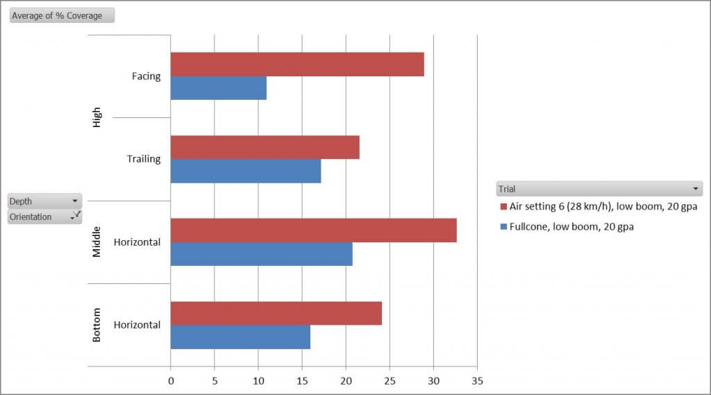
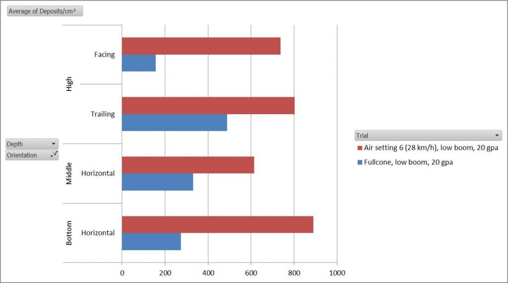
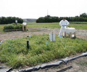
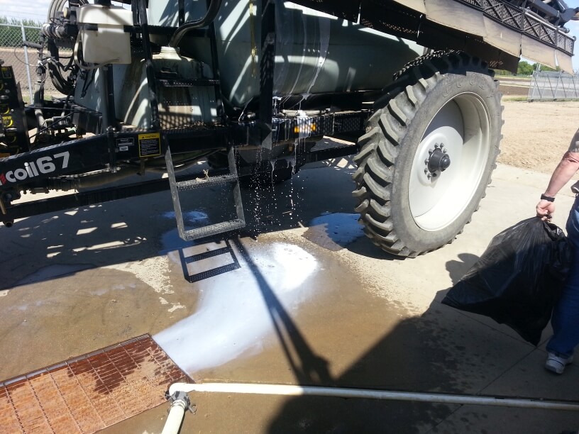
    Figure 1: Sprayer fill station

    At Sprayers101.com, we’ve tried to tackle the problem by finding ways to generate less waste (Express End Caps, Accu-Volume), by disposing of the rinsate by spraying it out, or by installing an efficient continuous rinsing system. We’d now like to talk about another component, biobeds.

    What is a biobed?

    Simply put, a biobed is a place where it’s safe and acceptable to dump dilute pesticide waste. First implemented in Sweden about 20 years ago, a biobed typically consists of a 1-m deep pit measuring about 3 m x 6 m or so. The pit is filled with a biomix, a mixture of cereal straw, compost or peat, and soil. The biomix, when properly prepared, acts to absorb a large amount of moisture, adsorb the pesticide molecules, and provide an environment in which microbes break down the residues.

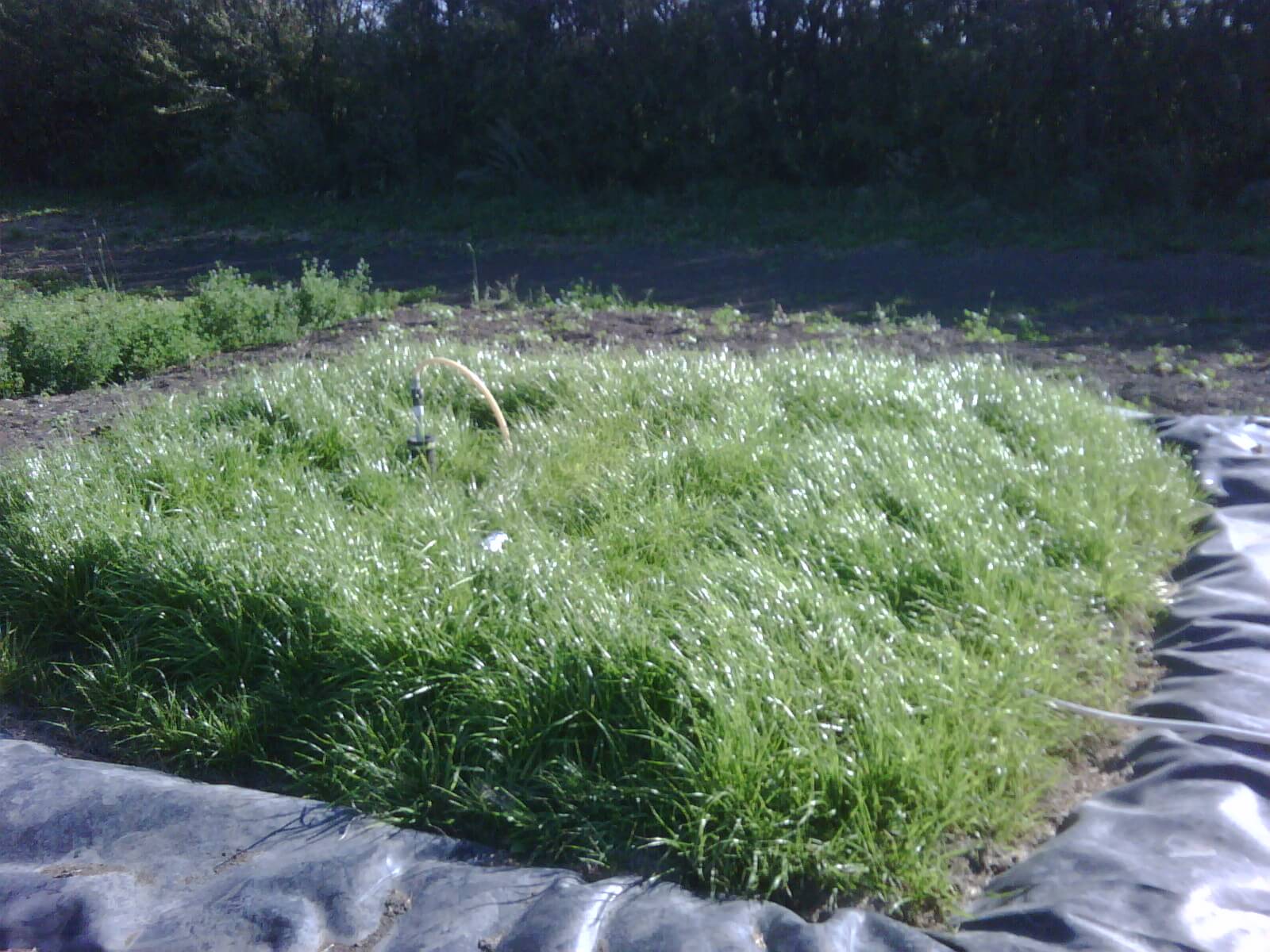
    Figure 2: Canada’s first commercial biobed installation at Indian Head, SK, 2009 (Source: Murray Belyk, Bayer CropScience (retired)).

    The effluent from a properly constructed biobed system contains 90 to 99% less pesticide than what was introduced, depending on the pesticide.

    Biobeds have been extensively studied and are now found throughout Europe and many parts of Central and South America. Canada currently has 6 research biobed sites in the West, and a further 17 in Quebec. The systems have been researched by Agriculture & Agri-Food Canada (AAFC) in recent years, with promising results.

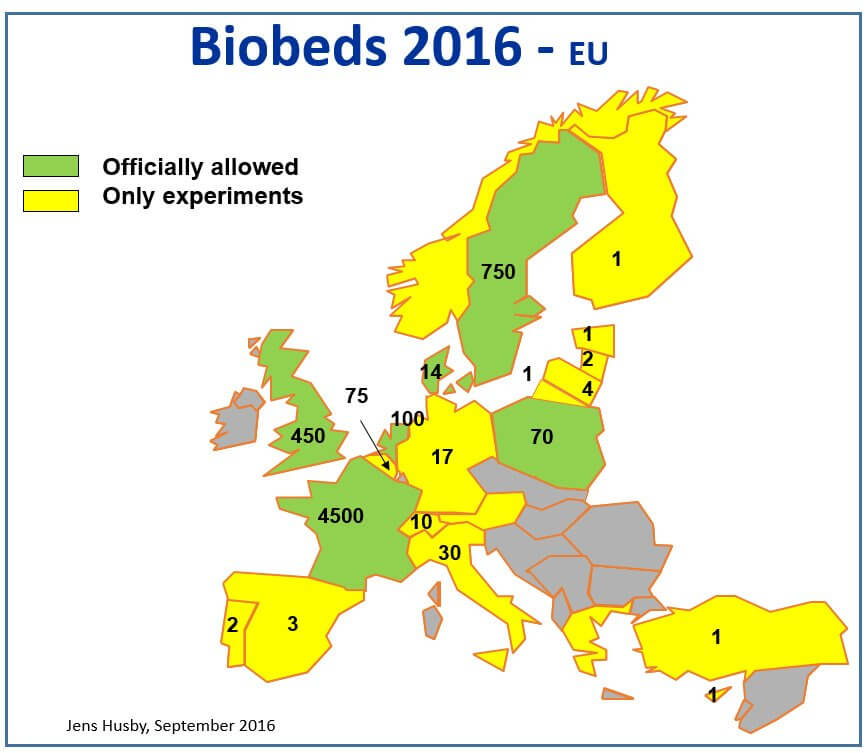
    Figure 3: European biobed installations, 2016 (Source: Jens Husby, Biobeds.org).

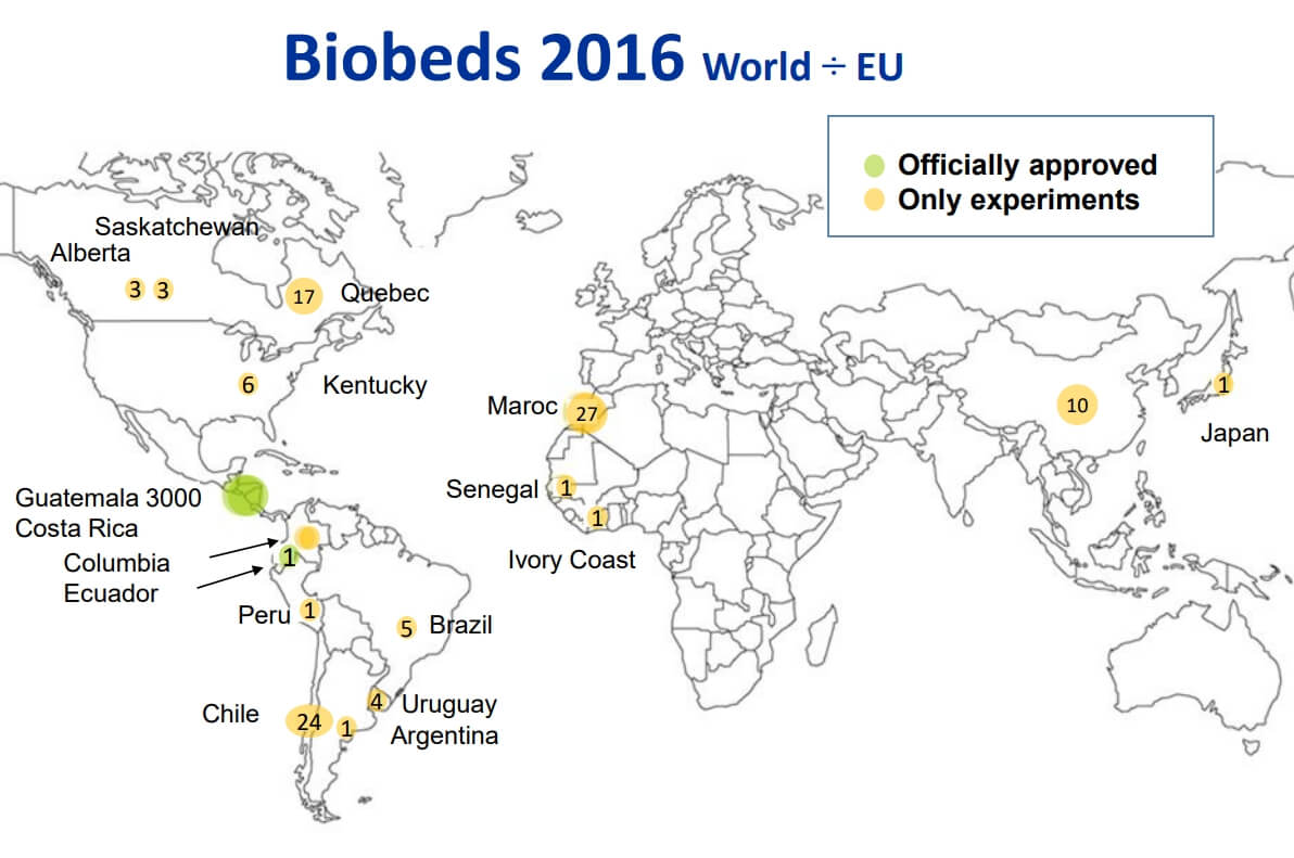
    Figure 4: Global biobed installations, 2016 (Source: Jens Husby, Biobeds.org).

    Constructing a biobed

    There are many possible variations of biobeds, some relatively simple and others engineered to address certain specific needs. A great deal of creativity can be used to customize a biobed for any operation.

    A simple biobed

    The following is a variation of the simplest biobeds, and these are the types first tested by AAFC in Saskatoon and Indian Head, Saskatchewan about 10 years ago. This design is based on the biobeds established in Sweden and the UK, and is a good way to learn about the system.

    Note that this biobed has an impermeable liner, so it’s a closed system. Excess water that leaches to the bottom must be removed and cycled back to the top of the biobed.

    • Create the biomix by blending two parts, by volume, chopped cereal straw or wood chips (not cedar), one part mature plant-sourced compost or peat and one part relatively coarse-textured soil (for optimal drainage). Add water as necessary as if making compost. Allow to sit for four to six weeks.

    Figure 5: Biomix preparation.

    • During this waiting time, the biomix will warm and form a white-mold complex. This is the microbial basis for its ability to break down pesticide residues. White mold will be visible on the cellulose portions of the biomix.

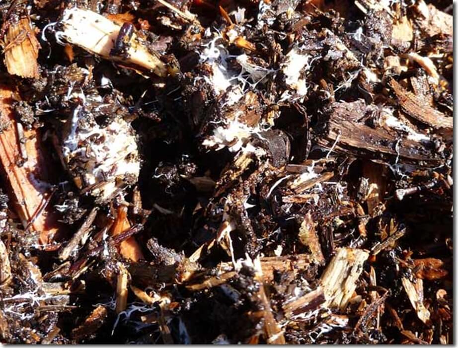
    Figure 6: white mold (Source: AAFC).

    • Identify a well-drained site easily accessible by spray equipment. Avoid low spots as water management becomes problematic.

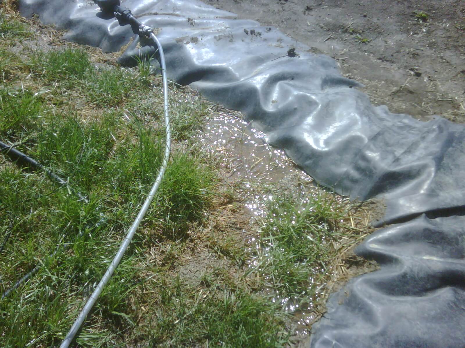
    Figure 7: Site selection and/or biobed covering are essential to avoid waterlogging (Source: Murray Belyk, Bayer CropScience (retired)).

    • Dig a pit sized to suit your requirements. As a rule of thumb, 1 m3 can process about 1000 L of liquid in a season. Rainfall is included in this amount.

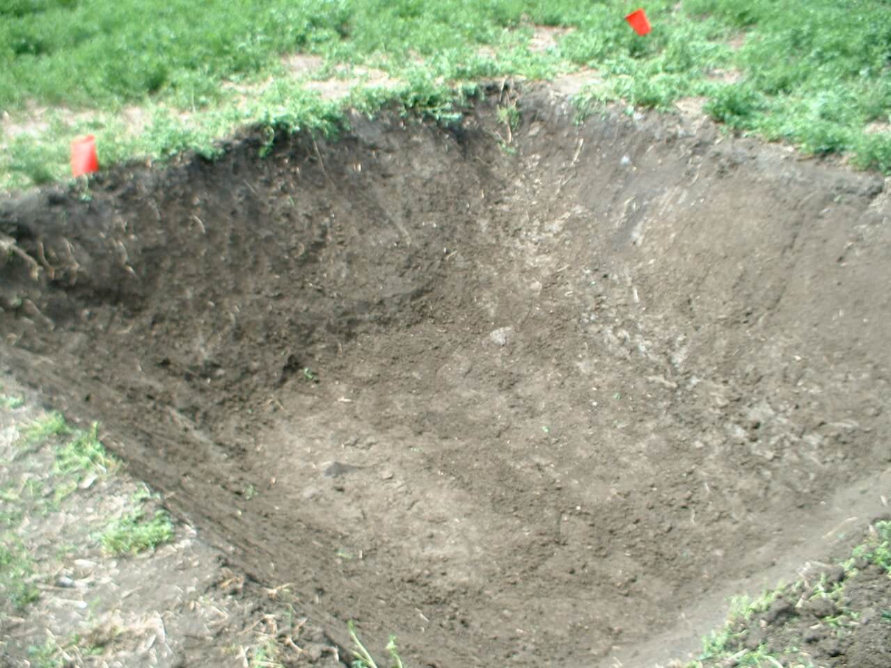
    Figure 8: A nice looking pit.

    • Line the pit with a geomembrane liner. 40 mil is plenty thick; any thicker and it gets hard to handle. Include a raised berm at the edge.

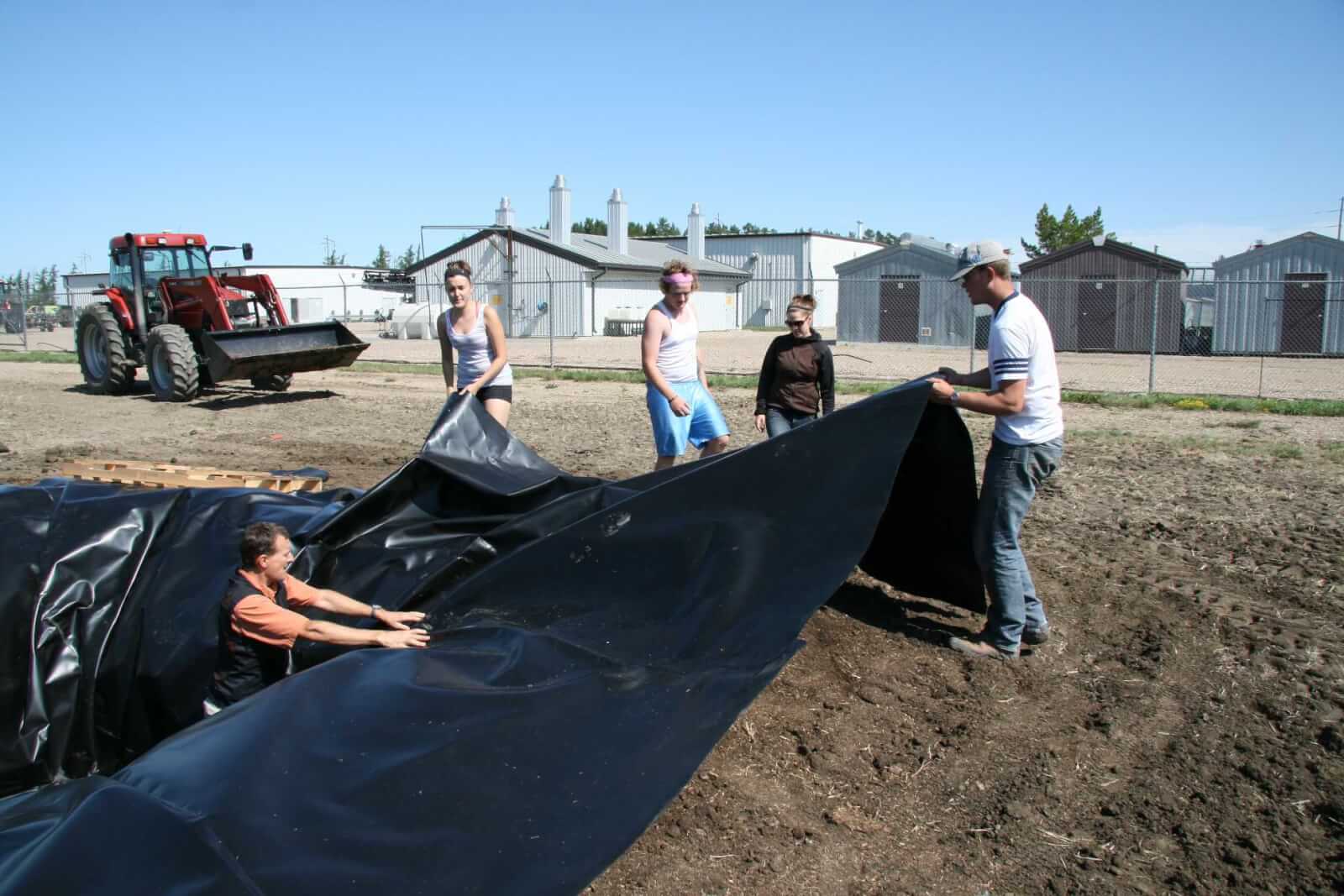
    Figure 9: Liner creates a closed system that will require a way to remove leached water.

    • Install weeping tile at bottom of pit, and extend it to ground level. This will be useful to determine water status and remove water if necessary.

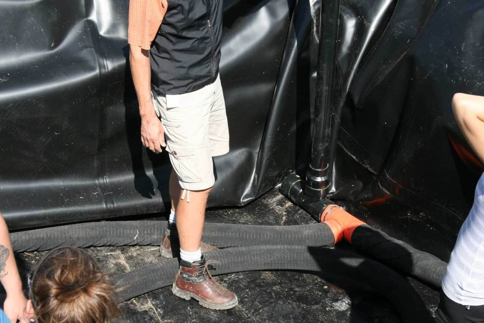
    Figure 10: Weeping tile to collect excess water.

    • Cover weeping tile with pea gravel and a silt trap. This serves to make leached water freely available for removal.

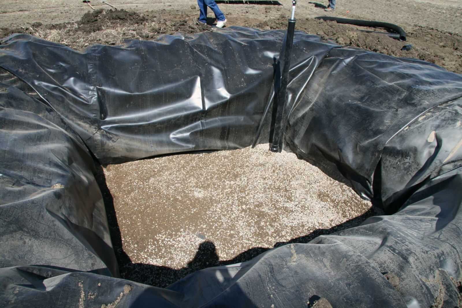
    Figure 11: Pea gravel over weeping tile.

    • Fill pit with biomix, anticipating significant settling. Top up as necessary over next few weeks. Use extra biomix to create a slope away from berm.

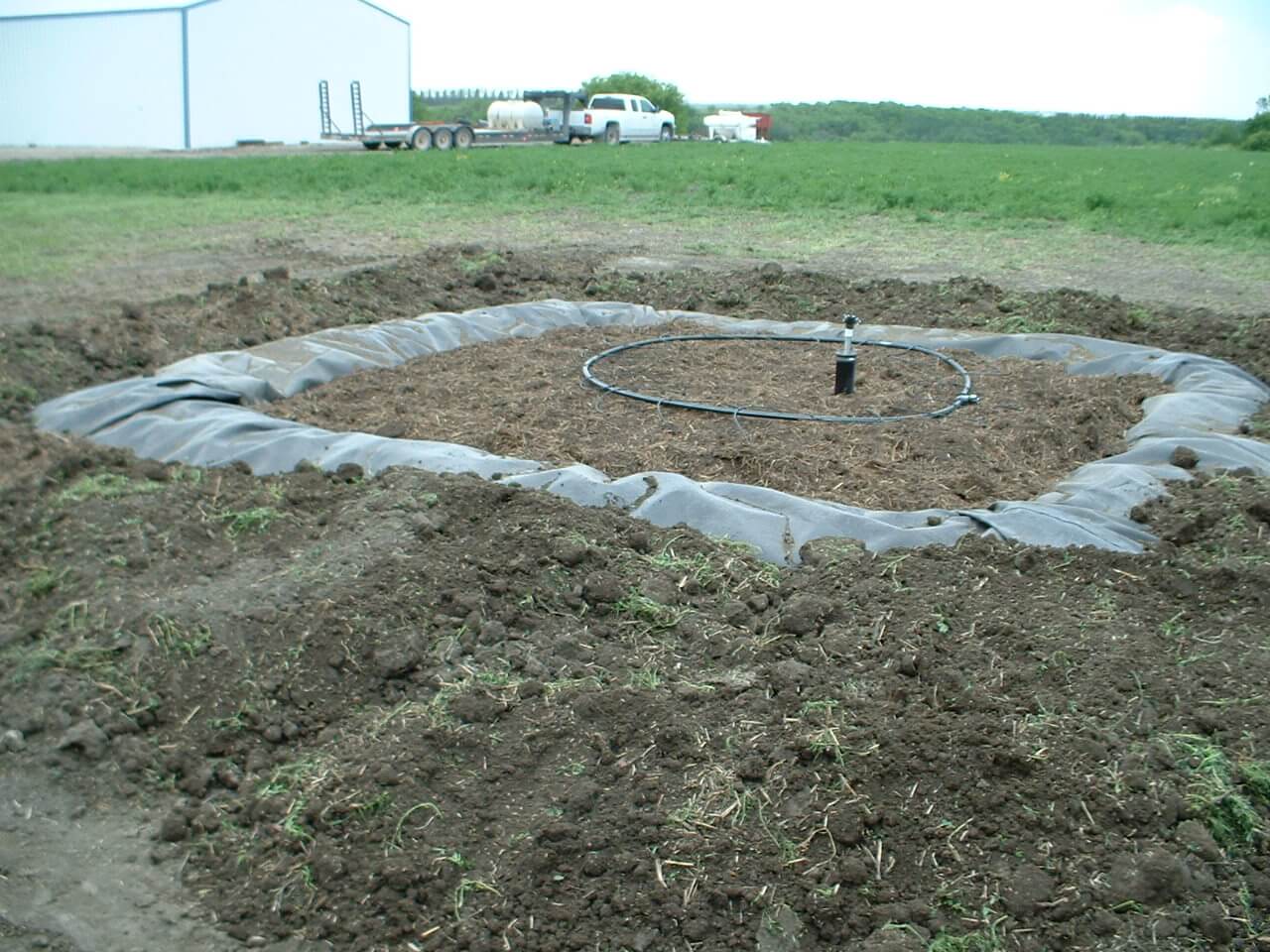
    Figure 12: Filled biobed.

    • Establish a bromegrass cover by transplanting or sodding. This is an important way to remove excess water via evapotranspiration.

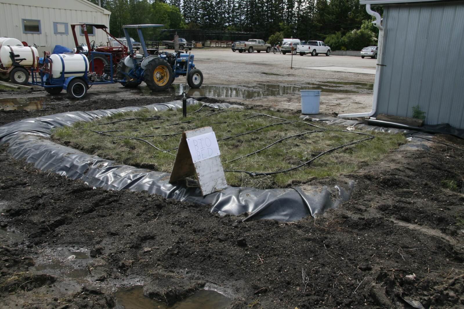
    Figure 13: Early sod growth on biobed at Indian Head, SK.

    • Introduce pesticide waste to biobed, managing moisture content to avoid waterlogging.

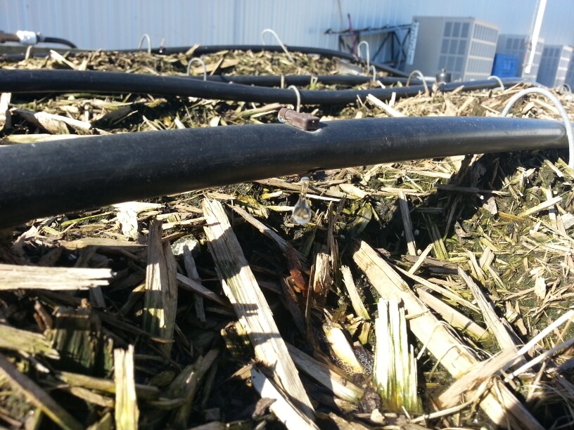
    Figure 14:  Pesticide waste entering biobed via drip irrigation.

    Introduction of pesticide waste to the biobed

    Moving pesticide waste from the sprayer to the biobed should be easy and trouble free. A simple pad built beside biobeds, either sealed with concrete or asphalt, or with a hardy geomembrane liner, works well. The sprayer is cleaned on this pad and rinsate flows into a drain. A sump pump lifts the rinsate to a storage tank from which it is introduced via gravity or pumped drip irrigation.

    Figure 15: Biobed system in Simpson, SK. Rinsate from sprayer is collected in a sump, which is pumped to the black storage tank in background. Rinsate is introduced into biobed (blue tub) as needed (Brian Caldwell in foreground, left, Larry Braul, right).

    When not in use, the sump drains freely to dispose of rain water.

    Others choose to pump or dump rinsate directly into a holding tank, from where it can be pumped onto the biobed.

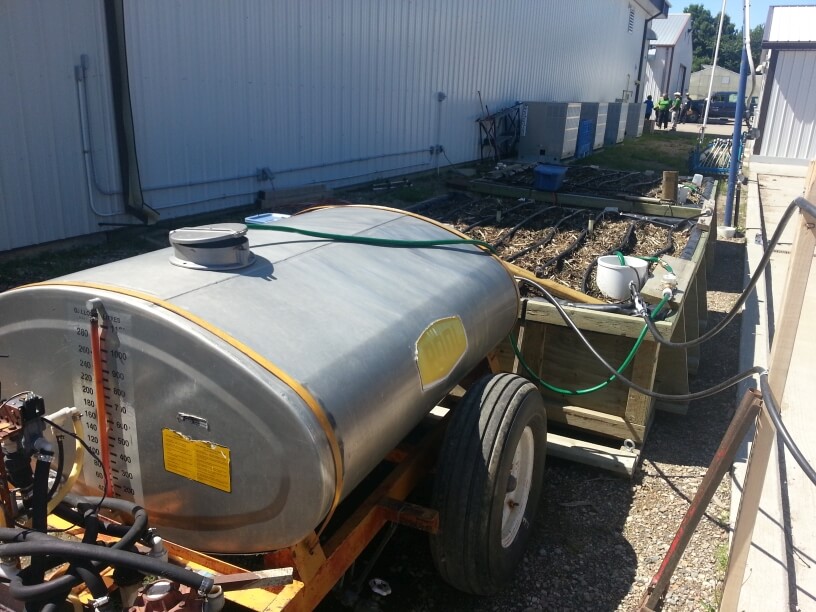
    Figure 16: Holding tank at biobed in Outlook, SK.

    Some European systems include driving supports on the biobed so the sprayer can be parked directly over top.

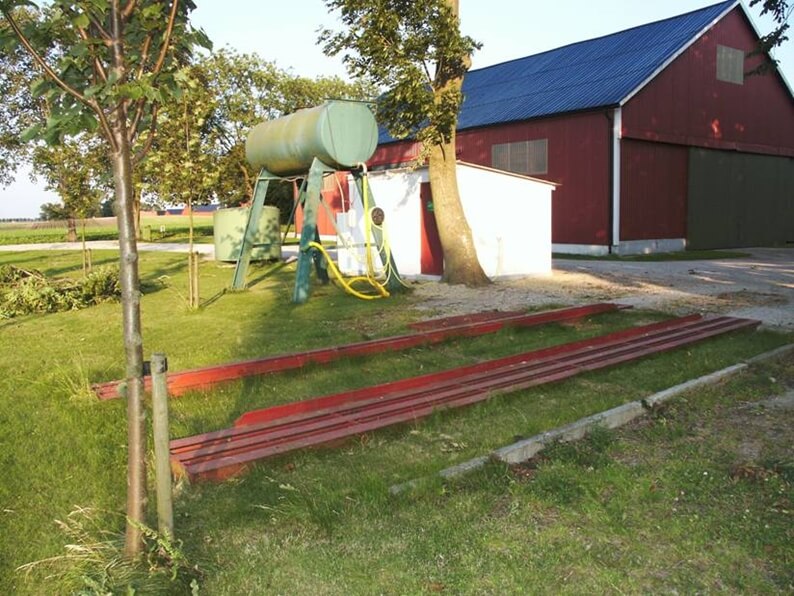
    Figure 17: Steel beams can allow (light) sprayer access (Source: Eskil Nilsson via Biobeds.org).

    A two-stage biobed

    The same basic building principles apply as in the original simple biobed. However, instead of reintroducing the effluent to the top of the biomix as it collects on the bottom, it is instead pumped onto a second biobed. This biobed then degrades any remaining product. This system is more efficient at degrading persistent products, and allows for better water management.

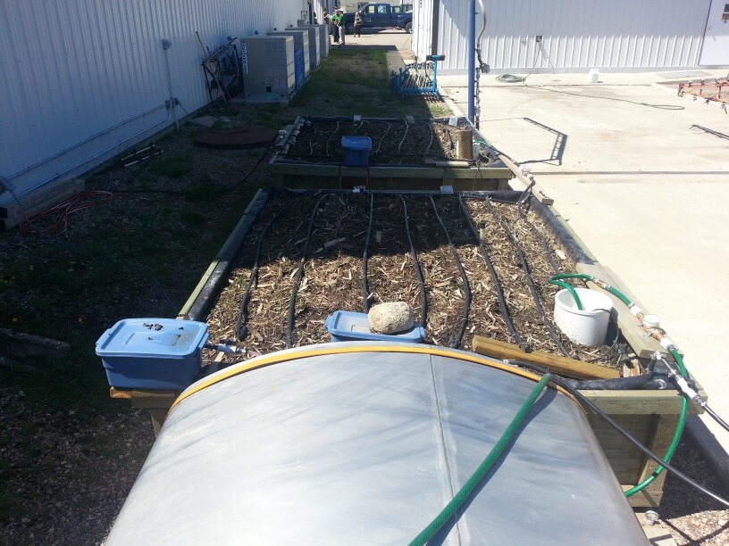
    Figure 18: Two-stage biobed system at Outlook, SK.

    The principle has proven effective, helping degrade more difficult pesticides to acceptable levels.

    Above-ground biobeds

    One of the problems with below-ground biobeds in wet climates is the difficulty managing water. Above-ground biobeds can address this issue by eliminating the possibility of surface runoff being added to the biomix. Adding a rain cover would also be easier and more effective.

    Above-ground biobeds can be edged with plywood, or placed entirely into plastic tanks whose tops have been removed.

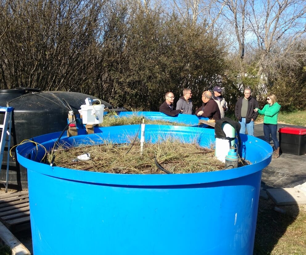
    Figure 19: Above ground biobed installation with plastic tub.

    One potential problem with above-ground biobeds is the later spring warming of this installation compared to below-ground types. Cold temperature reduces the effectiveness of biobeds due to the reliance on microbial activity. Heat tape has been tested by AAFC and shown to be very effective at warming the biomix and stimulating initial microbial activity. Passive solar systems have also been studied but are more difficult to install.

    Figure 20: Heat tape (Source: AAFC).

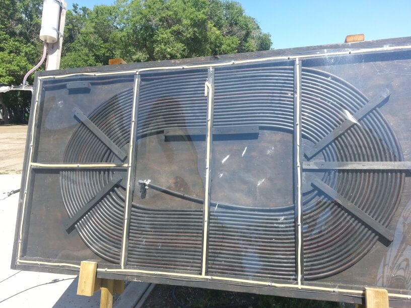
    Figure 21: Passive solar biomix heating system.

    Phytobac and Biofilters

    European designs have utilized plastic containers to form of various designs, including the commercial “Phytobac” systems from France and developed with the support of Bayer CropScience.

    Sequential biofilters have also been implemented. The leachate simply migrates through the biomix into the next container below. Eventually, adjacent biofilters containing plants act to remove the moisture.

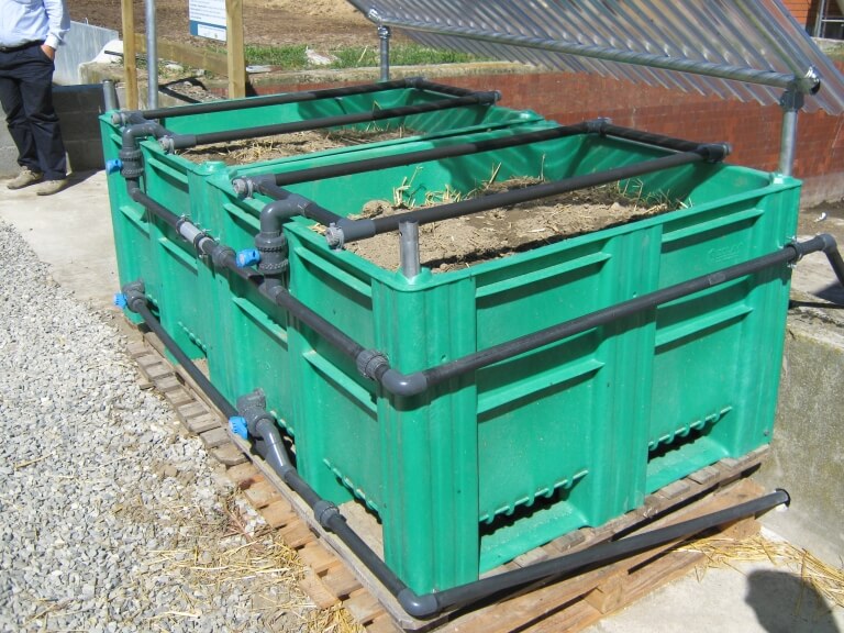
    Figure 22: Phytobac installation, cross-section.

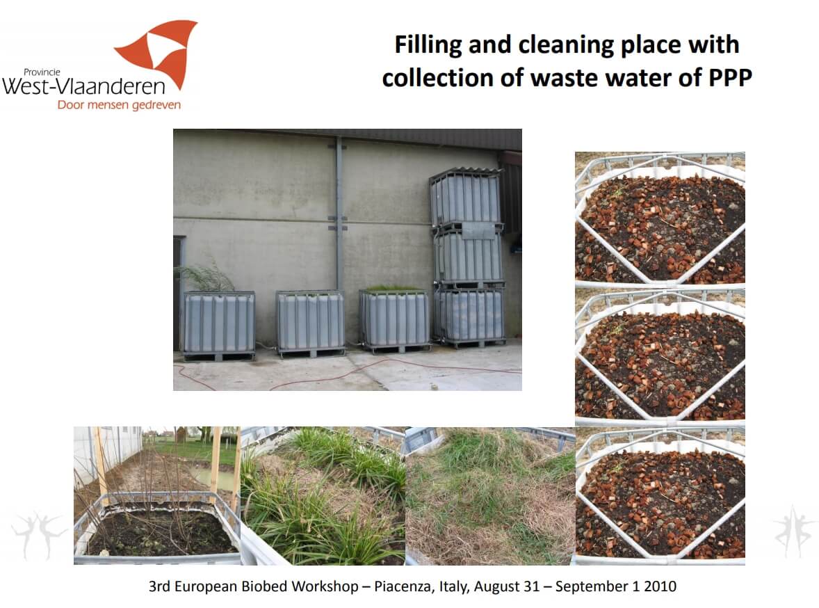
    Figure 23: Biofilter installation in Belgium (Source: Inge Mestdagh via Biobeds.org).

    Biomix longevity

    Swedish and UK research has suggested that biobeds require minimal maintenance aside from water management in closed systems. Biomix will settle over time and may need to be topped up. After five to eight years of use, it has been recommended to remove biomix and distribute it over a field with a manure spreader.

    Canadian research results

    Extensive analysis of pesticide degradation in five biobeds across Western Canada was conducted as part of a three-year study led by AAFC. Between eight and 51 products were analyzed per site, including herbicides, fungicides, and insecticides. Their results showed that single biobeds could remove about 90% of the introduced pesticide, and two in sequence usually removed more than 98%.

    Pesticides that tended not to degrade rapidly were removed to a greater degree in the second biobed.

    In the AAFC studies, three herbicides were more difficult to remove in the tested biobeds: clopyralid (e.g., Lontrel, Stinger), bentazon (Basagran, Storm) and imazethapyr (Pursuit, Arsenal). For these three, roughly 60% was removed in a two-biobed system.

    Concentrated pesticides should not be introduced to a biobed as this will kill the microbial populations.

    Some fungicides were shown to depress microbial populations but only temporarily. Microbial breakdown still occurred.

    Biobed manual

    AAFC has authored a comprehensive manual on biobed operation and installation based on research experience in Canada and elsewhere. It will be available here in late June 2018.

    The future of biobeds

    Research into biobeds remains active around the world. Different substrates for the biomix are being studied to suit local availabilities. Various systems, ranging from simple to highly engineered are being studied. Degradation effectiveness for various influents remains a topic of significant interest. Producer adoption and implementation are being reported.

    Thanks to funded research projects, biobeds are up and working at Canadian institutional sites such as government research centres, and there are opportunities for county and municipal government sites. For biobeds to be a viable option on North American farms, their design needs to remain simple and their integration into established practices needs to be seamless. Producer experience and feedback are essential

    Learn more

    Valuable information on biobeds can be obtained from these two websites:

    Voluntary Initiative (UK industry)

    Biobeds.org (International research)

    Note: Brian Caldwell and I first learned about biobeds from Eskil Nilsson (website) during a visit to Sweden in 2001, and obtained support for initial studies in Saskatoon and Indian Head from the Pest Management Centre as well as Bayer CropScience. Brian took a lead in our creative and technical efforts over many years. Dean Ngombe, under the co-supervision of Diane Knight at the U of S and myself, produced the first M.Sc. thesis, and with significant input from Allan Cessna, the first scientific publications in Canada on biobeds. Thanks for Larry Braul and many collaborators for leading the most recent AAFC study and generously sharing resources, and Erl Svendsen, Bruce Gossen, and Claudia Sheedy for editorial input.

  • Plot Sprayer Calibration Worksheet

    Plot Sprayer Calibration Worksheet

    Need a worksheet for calibrating a plot sprayer? Well, we just so happen to have one here:

    Plot Sprayer Calibration (May 15, 2018)