Author: Tom Wolf

  • Does the Pull-Type Sprayer once again have a Place on our Farms?

    Does the Pull-Type Sprayer once again have a Place on our Farms?

    The self-propelled sprayer revolution is complete in western Canada. Almost all sales of new equipment are self-propelled. In fact, the once thriving sector of Canadian-made pull-type sprayers, and the innovations they brought to spraying, has disappeared.

    In its place we have self-propelled sprayers that offer plenty of power, large tanks, high mobility and comfort, and of course, the clearance required for late-season sprays. These features come at a cost: high capital expense, weight, fuel consumption and drift potential if the speed or boom height are not controlled.

    The self-propelled machines are nice; however, customers are becoming concerned about overall value. Sure, the sprayer is the most-used piece of equipment on the farm, with the average field being treated four to five times per year. Does that justify the $500 to $700 k purchase price?

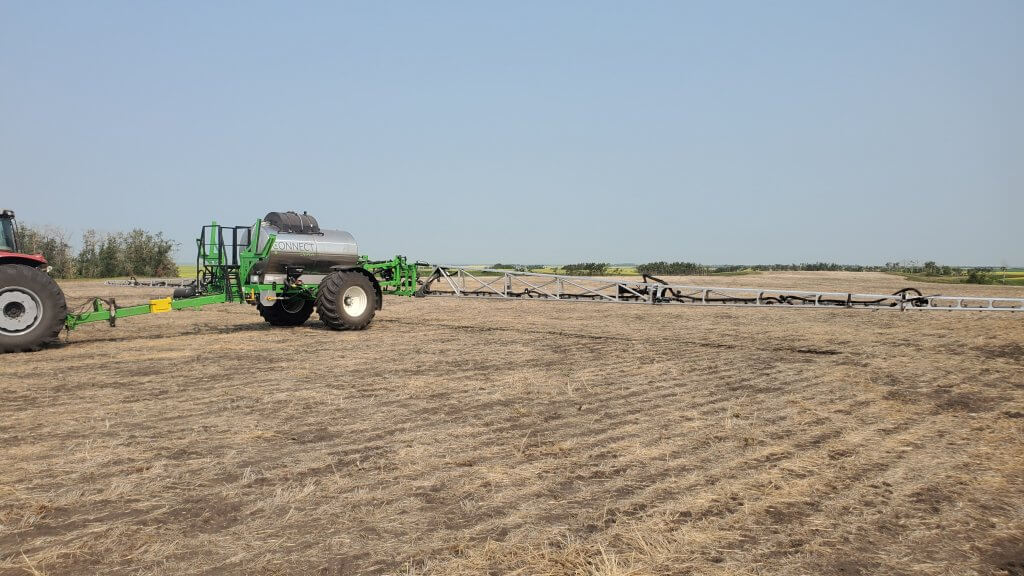
    To answer this question, we need to evaluate the alternatives. Even though we’ve lost most North American pull-type sprayer makers, a few, such as Top Air, are left. A new pull type, the Connect Sniper, is being offered by Pattison Liquid. In addition, there are now several European manufacturers looking at our market. These bring large capacity, sophisticated booms plumbing and a narrow transport width. Let’s look at the issues:

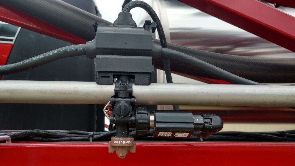
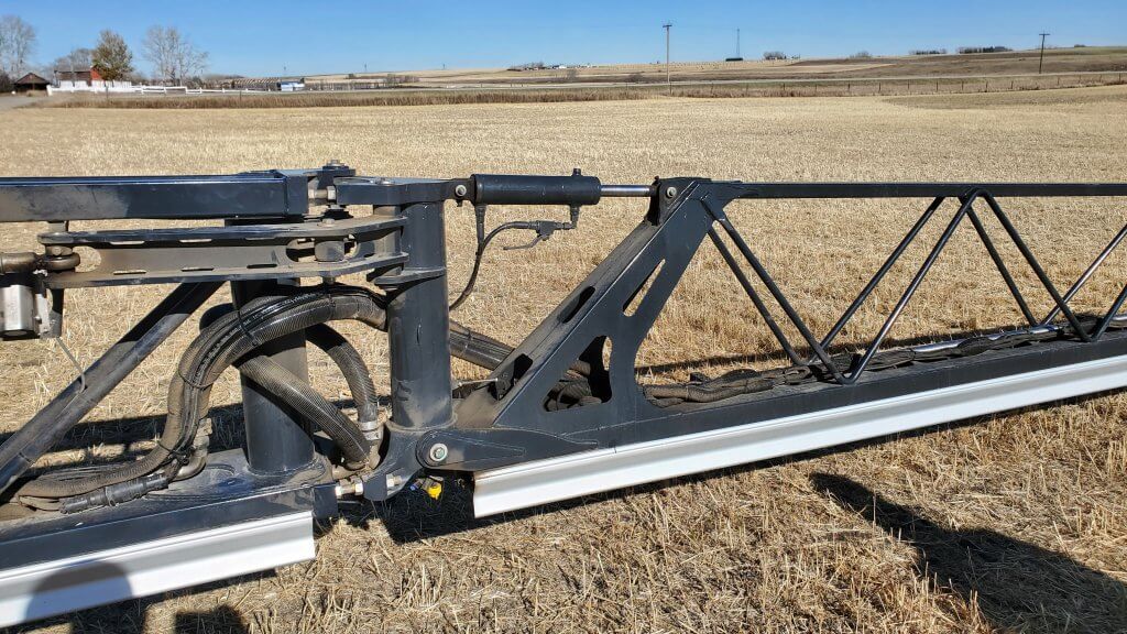
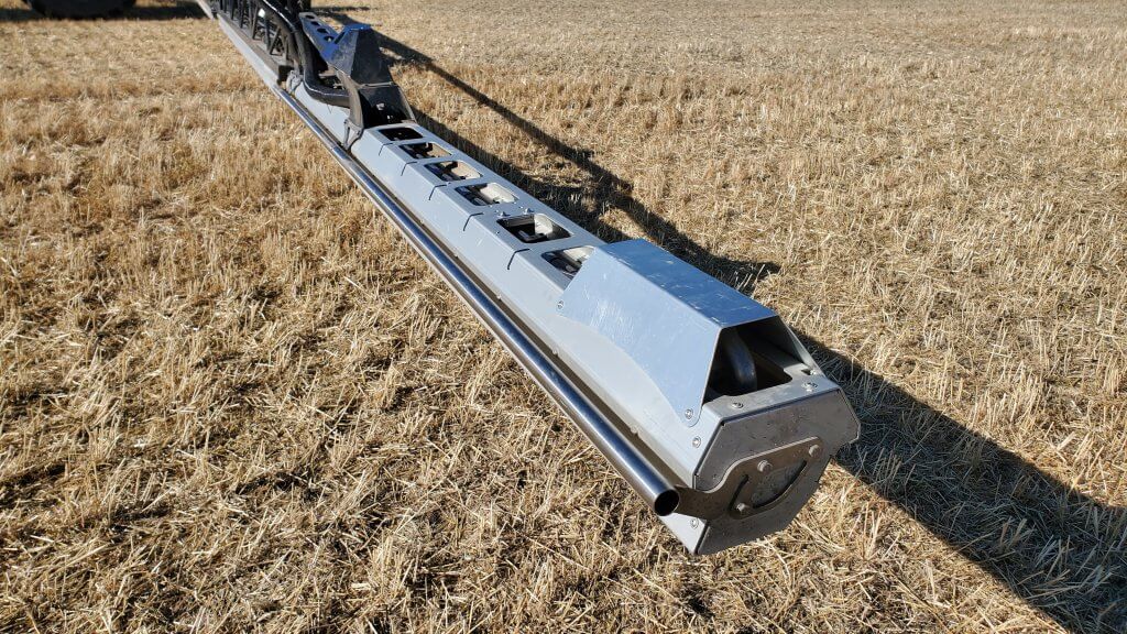
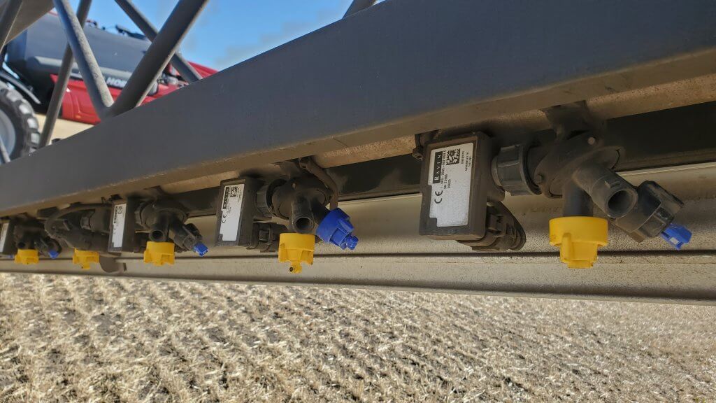
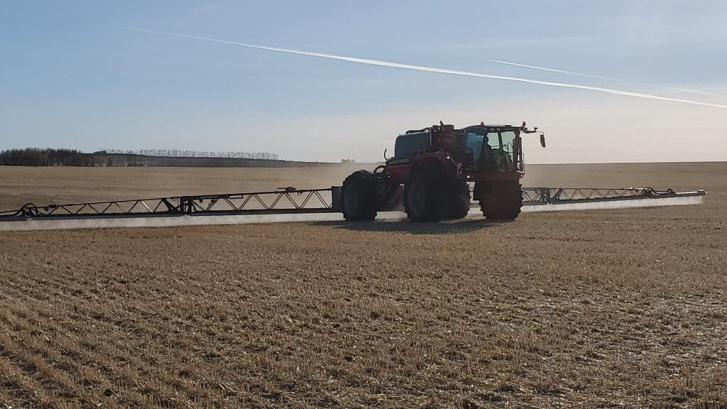
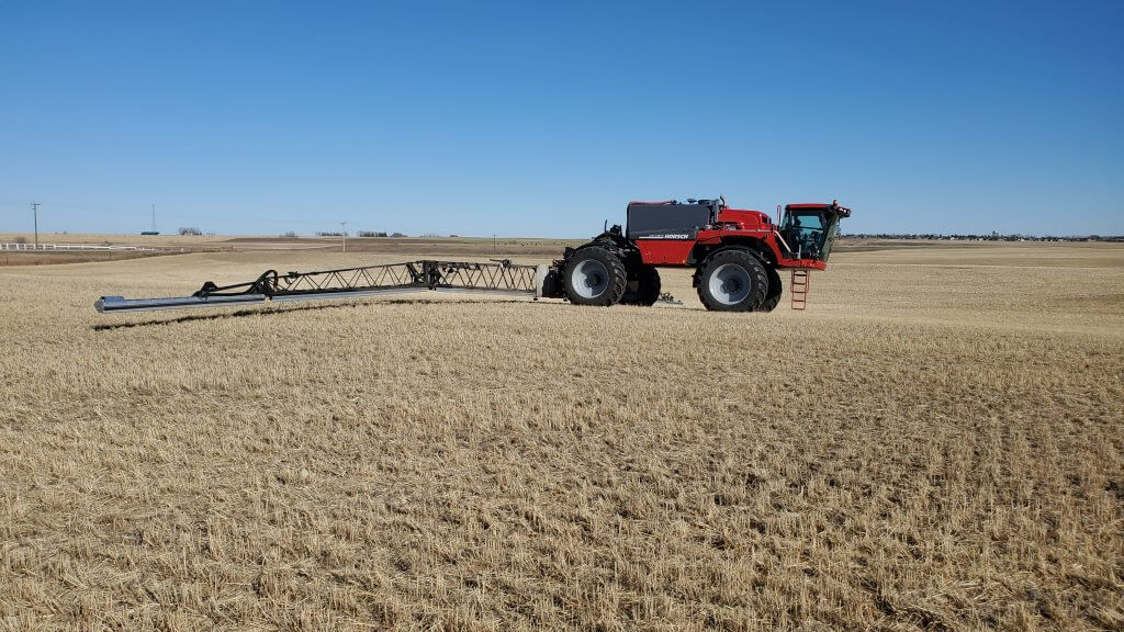
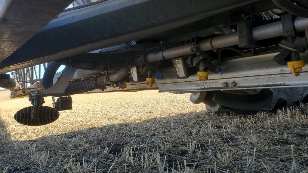
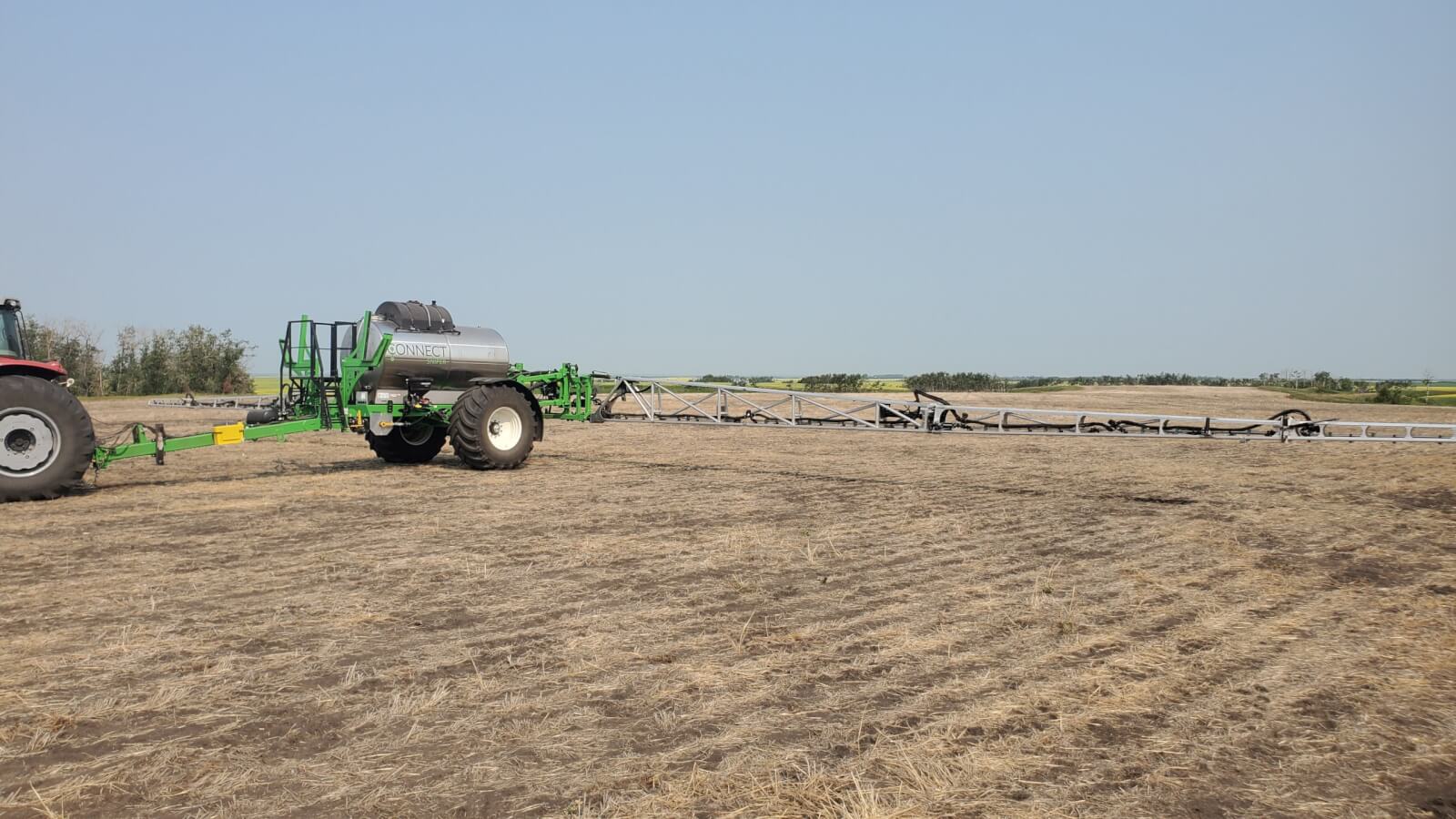
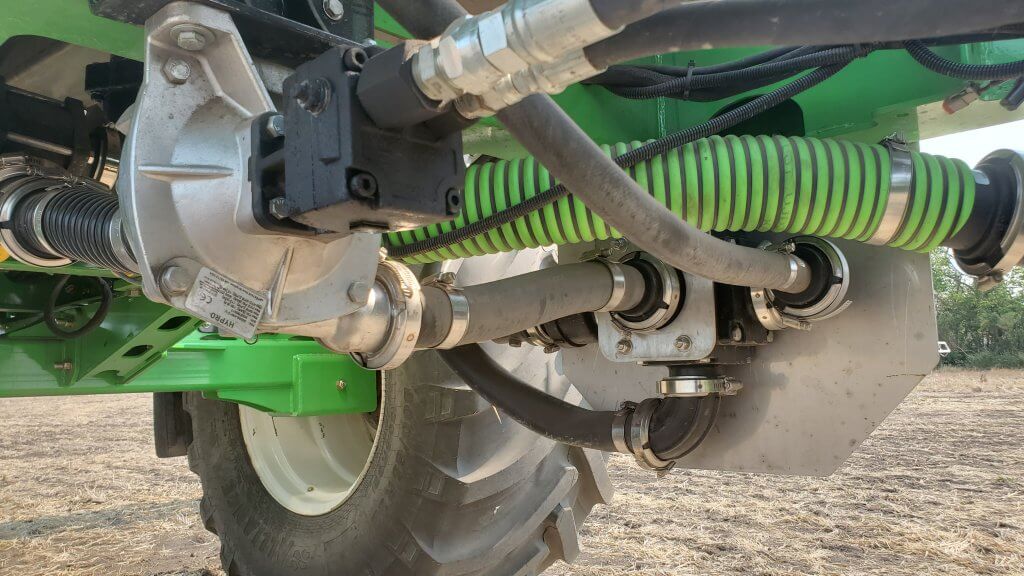
    The Connect Sniper, manufactured by Pattison Liquid, offers recirculating booms, Raven Hawkeye pulse-width modulation, continuous rinsing, and 120′ Millenium booms. The WEEDit spot spray system is also available.

    Capacity

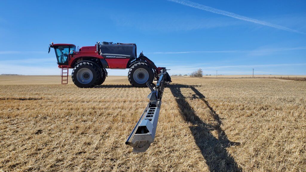
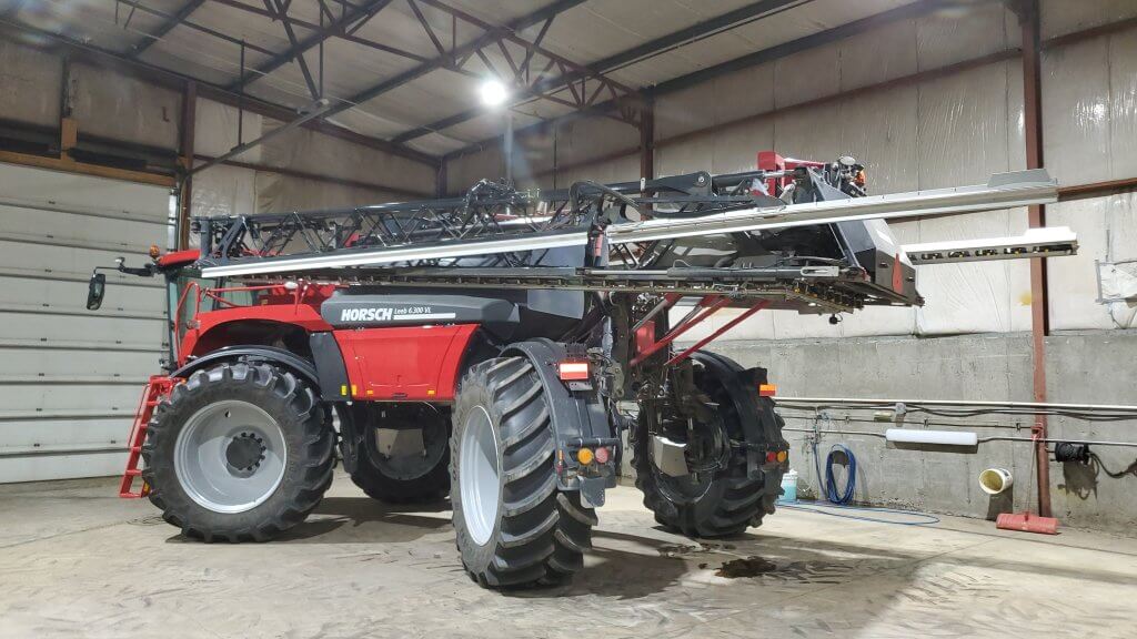
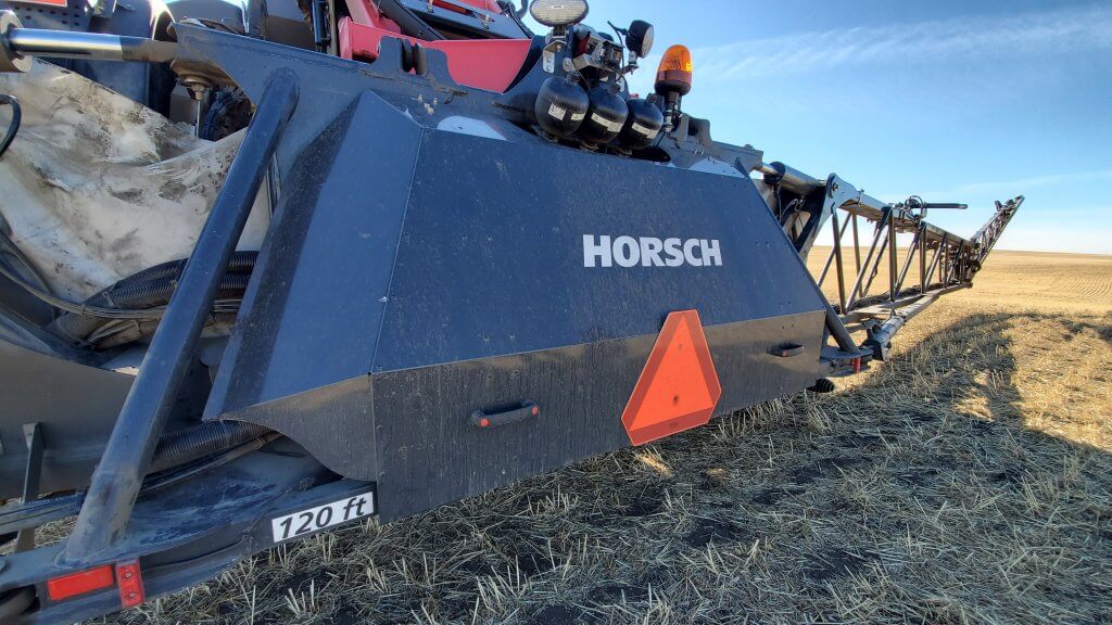
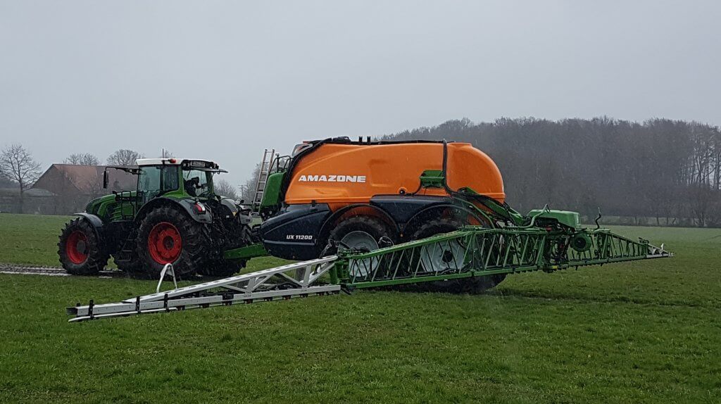
    Not a problem. Top Air features tanks up to 2400 gallons and 132’ booms. Amazone builds a 3000 gallon tank twin axle sprayer (UX11200) with 132’ booms. The 230 gpm on-board diaphragm pump can fill the sprayer in 15 minutes. The Hardi Commander offers tanks up to 2600 gallons with 132’ booms. The Horsch Leeb TD12 is at 3170 gallons with 138’ booms. Equipped with air brakes, these sprayers can be trailed at up to 50 km/h.

    The Amazone UX 11200 has an 11,200 L (2960 US gal) tank and tandem, steering axles combined with up to 130′ booms.

    Clearance

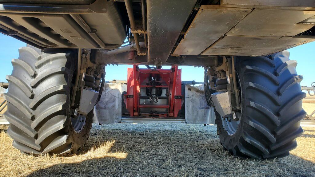
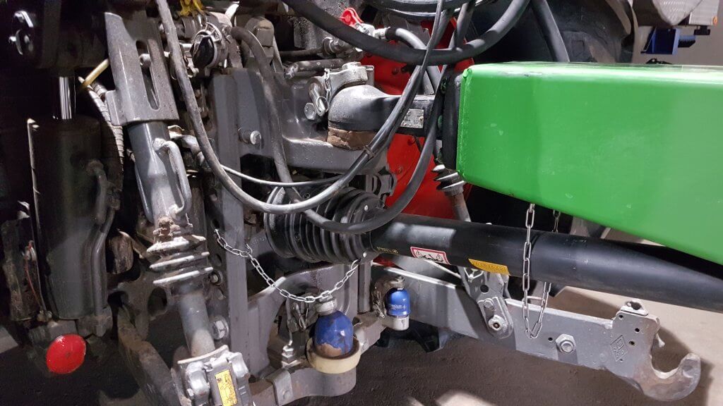
    The pull-types themselves have adequate clearance for most crops. The limiting factor will be the tractor and the hitch point. The availability of a high hitch point, and an 80 mm ball, on European tractors, is a boon for this.  Although it may be necessary to shield the low standard drawbar and belly, pull-type owners report no long-term effects from the lower clearance.

    The Horsch Leeb TD12 offers a 12,000 L (3170 US gal) tank and up to 1.25 m ground clearance (Photo: Horsch.com).
    European tractors offer 80 mm ball hitches for larger implements with high mounting heights to gain extra sprayer clearance.

    Tractor

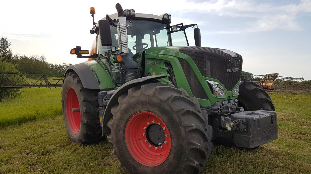
    The pull-type sprayer makes most sense if it allows the re-purposing of an existing tractor.  The common yard tractor isn’t enough, as the high capacity sprayers may require >200 hp with front wheel assist, especially in softer ground or hilly terrain. Another requirement is that the track width match the sprayer, and the European standard of a 2.25 m track width (centre to centre) can be hard to match in North America. New rims on the sprayer can push the width out, but the resulting increased axle stress may be problematic; these issues should be considered in advance. Fortunately, powerful front wheel assist tractors are finding a place on farms, even as seeding tractors. The changing over from one implement to another during a busy time can be a hassle, with a dedicated rate controller requiring additional cab real estate. But with the lower capital cost of a pull-type, a new tractor that also has other utility on the farm may be justified.

    Large pull types require large tractors that may not already exist on the farm. The ability to match wheel tracks and the convenience of monitor hookups are important considerations.

    Productivity

    We’ve long maintained that productivity gain through increased travel speed creates more problems than it solves. It is virtually unavoidable to use somewhat higher booms with faster speeds, and it’s been proven that spray drift potential increases with travel speed. Instead, the sprayer features that save time are faster fill and clean times (reduced downtime), larger tanks (fewer stops to fill) and wider booms. Wider booms are easier to keep steady with slower moving equipment.

    So how do typical self-propelled sprayers stack up against pull-types?

    We compared two sprayers, a large pull-type with 3000 US gallon tank and a typical self-propelled with a 1200 gallon tank. Travel speeds were 10 and 15 mph, respectively, and fill times were 15 and 10 minutes. The slower pull-type turned in one headland, whereas the self-propelled used two to allow room for acceleration after the turn.

    On half-mile runs, our “Productivity Calculator” at agrimetrixapps.com showed 129 acres per hour for the self-propelled and a respectable 119 acres/h for the pull type.  The value of fast but infrequent fills and the more efficient turns made the difference for the pull-type.  Use the app to compare other tank sizes, travel- and fill-speeds, or boom widths.

    Productivity of a 3000 gallon tank pull-type (left) vs a 1200 gallon self-propelled (right), given specific speed, boom width, and fill times.

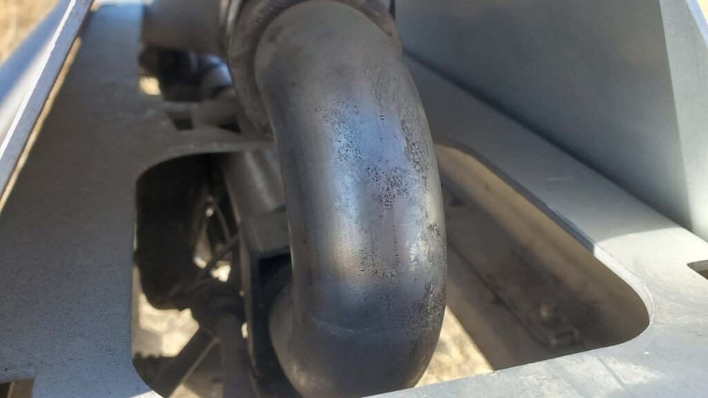
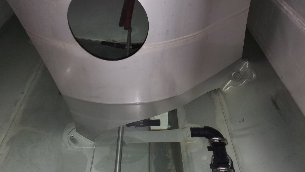
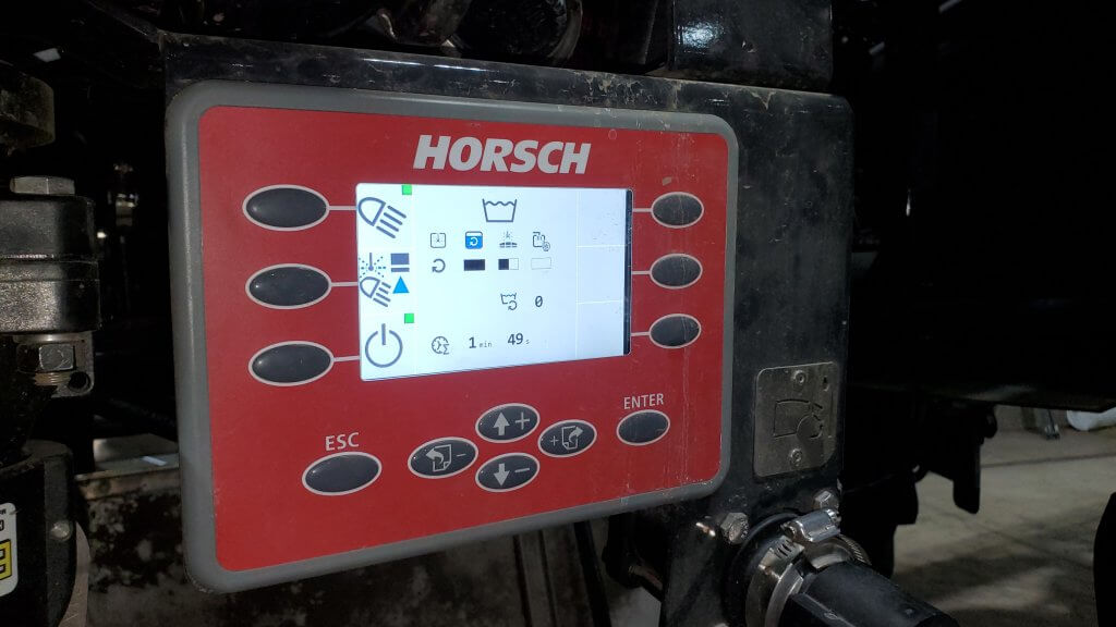
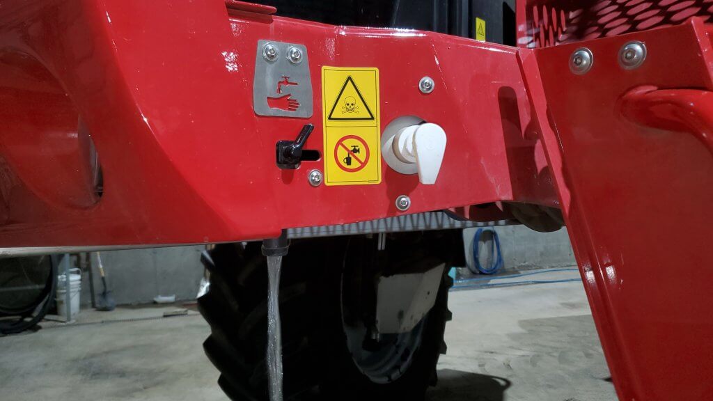
    The specific design features of a sprayer may create additional productivity. For example, the ease of tank rinsing and cleanout can save time. European sprayers typically have lower remaining volume values, which increases the speed of tank rinsing and can eliminate the need for dumping tank remainders on the ground. Ease of filter inspection may seem trivial, but it permits more frequent confirmation that the system is clean and thus avoids potential future problems.  An on-board pressure washer on the Amazone makes boom hygiene easier. It’s important to account for all these seemingly small gains because they add up.

    Service

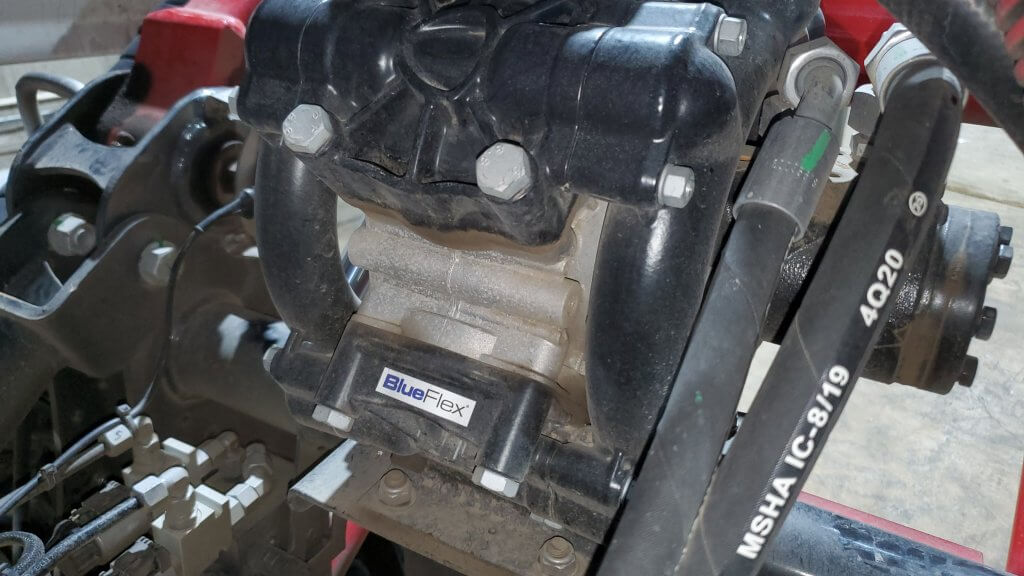
    The success of any agricultural equipment relies on the equipment durability, fast availability of parts and service. Any new market entry will need to establish a dealer network, parts distribution system and superior service. This is no easy feat in a time of dealer consolidation. But without a drive train, there’s less to go wrong in a pull-type, and many plumbing parts are generic or can be obtained in metric equivalents.

    With fewer mechanical components, pull-type sprayers require less service and are less prone to breakdowns.

    Cost and Value

    Prices vary, but a pull-type sprayer will usually cost less than half of a similar-sized self-propelled sprayer depending on the options selected.

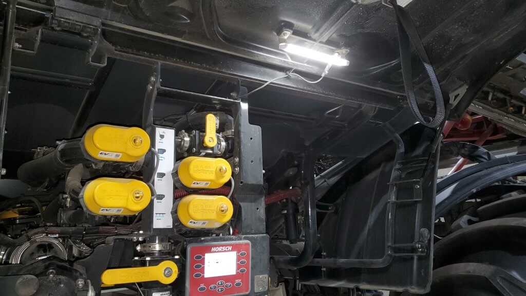
    With European-influenced equipment, the plumbing system will be more sophisticated, often offering recirculating booms, steering axles that follow in the tracks of the sprayer, narrow transport widths for greater road safety, an improved boom suspensions and levelling performance. It is safe to say that in terms of features, these sophisticated machines offer good value and many good design ideas. Operating costs are almost certainly lower, with better fuel economy and less drivetrain trouble.

    The pull-type sprayer continues to have an important place to fill on our farms. With trade and weather anomalies lowering farm income, farmers are wary of being over-capitalized. It is conceivable that lower-cost and feature-rich alternatives to self-propelled units will have a fit.  They certainly make sense on smaller farms that may not be able to utilize the full performance of a self-propelled, or on a larger farm that needs extra capacity but doesn’t want to bear the capital cost of a second expensive sprayer. The inherently slower working speeds allow for lower booms, less drift, overall improved deposit accuracy and uniformity. They’re worth a closer look.

  • Riparian vegetation or low-drift nozzles for water protection?

    Riparian vegetation or low-drift nozzles for water protection?

    Authors: T M Wolf, B C Caldwell and J L Pederson. Originally published in Aspects of Applied Biology 71, 2004, in expanded form.

    Abstract

    Spray drift deposition into water bodies may pose environmental and health hazards, and buffer zones have been suggested as a means of mitigating water contamination.  Field trials were conducted to determine the effect of nozzle type and riparian vegetation on spray drift deposition into wetlands.  Three riparian vegetative types, minimal vegetation (grass), low vegetation (willow shrubs), and high vegetation (aspen trees) were compared with open field conditions.  Spray was released upwind of wetlands with these riparian characteristics with conventional and air-induced low-drift nozzles.  Low-drift nozzles reduced drift deposits by about 75% in the absence of any vegetation, and by 88 to 99% when vegetation was present.  Dense willow shrubs resulted in anomalous downwind deposits, possibly because of air turbulence caused by low porosity characteristics.  By considering vegetation effects, a 15-m buffer zone could be reduced to 5 to 7 m for conventional, and 1 to 4 m for low-drift nozzles without increasing deposits at the edge of the sensitive habitat.  Both variables should be considered by regulatory bodies in their risk assessment procedures.

    Introduction

    Airborne transport is an important vector for movement of pesticides from agricultural land to receiving waters.  In an effort to maintain low pesticide levels in water bodies in accordance with risk assessment protocols, the Pest Management Regulatory Agency (PMRA) is mandating minimum setback distances (buffer zones) from water bodies during a spray operation.  Several additional variables can complement buffer zones in preventing spray drift, including low-drift sprays and riparian vegetation.  Germany and the United Kingdom already account for these characteristics in their buffer zone regulations (Kappel and Taylor, 2002). 

    Vegetation has been shown to be effective at mitigating droplet spray drift in several recent studies and reviews (Richardson et al., 2002, Hewitt, 2001, Ucar and Hall, 2001) by reducing wind velocities and intercepting spray. The documented magnitude of the spray drift deposit reduction in these studies ranges from 50 to >95%, dependent on variables that include vegetation height, porosity and orientation relative to wind direction, and wind speed. 

    We studied the integrated effect of buffer zones, vegetative barriers, and low-drift sprays to determine the overall impact of spray drift deposition onto downwind water bodies.

    Materials and Methods

    Overview and Site Description

    The study was conducted in 2001 on a farm field near Aberdeen, SK. Sprays were applied upwind of a water body, and drift deposits were collected on petri-plates placed near ground level.  Experimental sites were chosen to represent different vegetation heights and types around the water body in question: low (uncut grass), intermediate (willow shrubs), and tall (aspen trees).  These were compared to nearby open-field conditions.  Two sprayer nozzle types were used in the study: conventional flat fan nozzles and venturi-type low-drift nozzles.

    The grass barrier was comprised of a mix of grasses dominated by bromegrass (Bromus spp.) growing to a height of 75 cm.  Willows (Salix spp.) were approximately 3 m tall with a density of about 0.15 m-2 and presented a fully foliated barrier for their full height.  Willows extended for a width of about 7 m toward the edge of the water body.  Trembling aspen (Populus tremuloides Michx.) were approximately 8 m tall, with foliation beginning 1.5 m above ground.  Trees were present at a density of about 0.25 m-2 and extended for 8 m toward the water edge. 

    Figure 1: Site and sampler layout

    Spray Equipment and Application Method

    A Melroe Spra-Coupe 220 was used to make the applications.  This sprayer was equipped with conventional flat fan nozzles (XR8003) and air-induced low-drift nozzles (TD11003) at 275 kPa, producing ASABE Fine and Coarse sprays, respectively.  The spray boom was 10 m wide and nozzles were 75 cm above ground.  Sprayer travel speed was 12.9 km h-1, at which the application volume was 100 L ha-1.

    The sprayer tank contained a mixture of 2,4-D amine4 (4 g L-1) and Rhodamine WT5 (2 mL L-1), a fluorescent tracer dye which would be used to quantify the deposits.  2,4‑D acted to photostabilize the dye, and also provided a spray formulation with physico-chemical properties representative of agricultural pesticides.

    Top row: Fine and Coarse sprays used in study
    Middle row: Tall and medium vegetation
    Bottom row: Short vegetation and open field

    Application was made in a direction approximately perpendicular to the prevailing wind, with the downwind edge of the spray boom at the edge of the wetland’s riparian vegetation.  This was usually about 15 m upwind of the edge of the water body (due to severe drought conditions, the wetland did not contain any water at the time of the trials).  Three consecutive passes were made along the same swath in a 10-min period to obtain average meteorological conditions for all three vegetation types.  Wind speed and direction, temperature and relative humidity were monitored during application using a portable micrometeorological station. 

    Sampler Layout

    Downwind of the spray swath there were 3 parallel lines of eleven 15-cm diameter glass petri-plate samplers starting underneath the sprayer boom and extending 46 m downwind from the edge of the spray swath (Figure 1).  Samplers were separated by 5 m within the line, and lines were about 2 m apart. 

    The deposition profile was also assessed under open field conditions, using the same sampler layout but on crop land with no riparian vegetation.  These are referred to as ‘bare soil, or ‘reference’ samplers in this report and served as a baseline to determine the impact of the riparian vegetation. 

    Sample Collection and Analysis

    Sample collection began 5 minutes after spray application was complete (See Table 2 for trial times).  Beginning with the furthest downwind locations, petri-plates were covered with a plastic lid, and placed into dark boxes.  Spray deposits on the samplers were washed off in the laboratory using 95% ethanol in three 15-mL washes.  Final samples were made up to 50 mL. and two 20-mL sub-samples were collected in borosilicate vials and stored in the dark. 

    Within 24 h, subsamples were analyzed using a fluorescence spectrophotometer with excitation and emission wavelengths of 545 and 570 nm, respectively (Shimadzu Model RF-1501 spectrofluorometer equipped with Model ASC-5 auto-sampler).  Instrument readings were converted to µg L-1 using standard curves and expressed as a percent of the applied dosage under the field sprayer. 

    The fluorescence spectrophotometer data were averaged over the three replicate sampling lines, adjusted for photolysis, and expressed as a percentage of the amount applied on-swath.  Relationships of spray drift deposits with downwind distance were first visualized by plotting all data points, and then mathematically related through appropriate regression techniques.

    Results

    Meteorological Conditions

    Weather conditions were favourable during the trials.  Wind speed and direction were appropriate for the sampler layout and the experimental objectives.  Mean wind direction varied by up to 44º from the ideal (270º) in 6 out of 12 trials, and was within 30º for the remaining 6 trials (Table 1).  Mean wind velocities were consistently between about 17 and 21 km h-1 in all but one trial.  Air temperature and relative humidity fluctuated between 14 to 22º C and 31 to 80%, respectively, on the trial dates.

    Deposition Profiles

    A visual review of the raw data suggested that a linear regression of the log of deposit amount and log of downwind distance would be appropriate.  It was noted that for willow, the deposit profile tailed upwards after the 26 m mark.  Based on a survey of the site, it was concluded that this tail was probably caused by the length of the spray pass exceeding the length of protection offered by vegetation.  In other words, beyond the 26 m sample, drift had not been attenuated by a vegetative barrier.  It is also possible that the airflow was deflected up over the low, non-porous barrier and returned to ground level beyond the 26 m distance (Carter et al., 2001).

    Figure 2: Spray deposit profiles from Fine (top) and Coarse (bottom) sprays.
    The deposition data for the willow were regressed from 6 to 26 m, all others were taken to 46 m (see text for explanation).

    As a result of the questionable data for this vegetation type, it was decided that it would be misleading to include the furthest downwind data points.  Implications of this observation will be discussed later in the manuscript.  All regressions were statistically significant, explaining between 61 and 99% of the observed variation.  In 5 of 8 trials, more than 90% of variation was explained. 

    Drift Mitigation by Riparian Vegetation and Application Method

    The predicted drift deposit at 15 m was calculated for all trials based on the regression parameters (Table 3).  For the conventional sprayer on bare soil, the deposit amount was 0.322% of the applied dose.  The distance at which this specific deposit amount would be achieved was then calculated for all other trials.  This value is the buffer zone distance at which equivalent protection to the reference system was offered.  Buffer zones could therefore be reduced by 55% (grass), 99% (willow) and 69% (aspen) using the conventional nozzle and 56% (bare soil), 74% (grass), 98% (willow) and 92% (aspen) for the low-drift nozzle. 

    Table 1: Buffer zone distances based on observed drift, calculated from regression.

    The calculated buffer zone reductions were not equivalent to the observed drift reductions due to the unique regression slopes of each deposition line.  For example, expected drift deposits at 15 m downwind on bare soil were reduced by 77% when the air-induced low-drift nozzles were used (Table 4), whereas buffer zone distances could only be reduced by 56% (Table 3).  Furthermore, the effectiveness of the grass vegetation diminished with distance, reducing drift by 64, 50, and 28% at distances of 15, 25, and 45 m, respectively.  Therefore, a complete deposition profile will be required for each vegetation scenario to accurately adjust buffer zones.   

    Table 2: Drift deposits expressed as a percent of the reference deposition line for two application methods, four vegetation types, and three downwind distances.  All numbers are the mean of three separate experiments on the same location. 

    Riparian vegetation was typically more effective than low-drift nozzles in protecting water bodies from drift deposition.  While grass reduced deposition by 28 to 64% from the conventional nozzle (depending on the downwind distance), willow and aspen reduced deposition by between 95 and 99% (Table 4).  The willow was not considered at further distances since the data used for the regression were truncated at 26 m.  Low-drift sprays provided some additional protection in all cases except for trees at the 45 m distance, where deposits increased slightly relative to the conventional spray. 

    Discussion

    The aerodynamics of vegetative barriers are a complex phenomenon.  Wind, upon reaching a solid barrier, is diverted up and over giving strongly turbulent conditions on the leeward side and a rapid return to free wind speed.  For a permeable barrier like a hedge, the return to free wind speed is more gradual since some air filters through, reducing the pressure differential and allowing for less turbulence (Davis et al., 1994).  Wind speed reduction is most pronounced for a distance of 5 H upwind and 30 H downwind at the 1 H height, where H is the height of the barrier (Rider, 1951). Nonetheless, there may still be an upward diversion of air (and spray drift) which may simply delay, not eliminate, sedimentation (Hewitt, 2001, Ucar and Hall, 2001), particularly for dense hedges (Carter et al., 2001).  Richardson et al. (2002) did not, however, notice such a deflection up to 10 m height. 

    The reduction in drift deposition by riparian vegetation in this study is clearly significant, but is subject to some interpretation.  These data were generated at a single site, and while this site was carefully selected to be representative and trials were repeated three times, it does not necessarily constitute an average result.  There are clearly any number of possible arrangements of trees, shrubs and grass, plus any additional vegetative or landscape features which would influence drift deposition behaviour.  However, due to the consistent nature of the data of this study, some confidence is attained in that the numbers are at least reliable for the given set of conditions.  In this study, three spray passes were made along the same swath at the edge of the water body.  Results could have been different had adjacent spray swaths been used, owing to the possible change in contribution of upwind swaths with the altered airflows under vegetated conditions. 

    Since the water body was dry, additional grass vegetation which had grown up could have made an effective collector of spray drift, possibly reducing deposit values beyond those that would have occurred in a water body.  It is recommended that efforts be made to repeat these studies when water is present at normal values. 

    The mitigating effect of vegetation depends on the aerodynamic features of the vegetation, as well as the collection efficiency of their leaves, twigs, etc.  This poses some difficulties because there are no absolute measures of these features.  Permeability, for example, varies with wind speed owing to the movement of leaves, and winds speed itself varies with height (Davis et al., 1994).  Collection efficiency of the vegetation varies similarly with target size, its movement, wind speed, and droplet size spectrum (Hewitt, 2001).  However, there are opportunities for improved characterization with specialized equipment, such as that used by Richardson et al. (2002).  Their LIDAR instrument was able to help calculate tree height and width, mean area index and mean area density. Work to further characterize vegetation will prove useful in future efforts to understand its mitigating potential. 

    Low vegetation such as grass has not received the recent attention of hedges and trees but has also been documented to reduce spray drift significantly.  A study by Miller et al. (2000) documented significant reductions in airborne drift concentrations above uncut grass canopies, even at low plant densities.  Bache (1980) documented similar reductions in spray drift when sprays were applied over a mature wheat crop compared to bare soil.  Therefore the filtering effects of “low” canopies may be very significant and should be the subject of further study. 

    Riparian areas are regions of high biological activity and diversity, not only protecting adjacent water from outside influence, but also providing food and shelter for many species of wildlife.  These areas must themselves be protected from harmful effects, which can include pesticides.  Their efficient capture of sprays suggests some risk from pesticides capable of controlling perennial vegetation.  Likewise, pesticide residues in this vegetation have the potential to be ingested by wildlife or be washed off with precipitation, resulting in movement into the water body.  These effects must be considered when using vegetation to mitigate airborne drift. 

    Conclusions and Recommendations

    • Vegetative barriers reduced spray drift deposition from conventional or low-drift nozzles into water bodies by 24 to 99%.
    • Low-drift sprays reduced deposition by about 75%.
    • Of the vegetation types, shrubs and trees had similar effects, reducing deposition from open-field conditions by an average of more than 95%.  Low-drift sprays improved on this reduction. 
    • Calculated buffer zone reductions were less than drift deposit reductions. Accurate determination of buffer zone distances requires that the entire deposition profile be characterized. 
    • It is suggested that both riparian vegetation and sprayer technologies are important components of water body protection.  Both should be considered in BMP and regulation development whenever the impact of pesticide applications near water bodies is to be estimated or mitigated. 

    Acknowledgements

    The technical assistance of Glenda Howarth, Jill Clark, Rachel Buhler, Murray Nelson, Trevor Linford, and Pam Reynolds is greatly appreciated.  Financial assistance was provided by the Rural Quality Program of the Agri-Food Innovation Fund, administered by the PFRA.  The authors wish to thank Darrell Corkal and Clint Hilliard of PFRA for their enthusiasm, support and guidance directed towards this project, and Raymond Malko for making his land available for the trials. 

    Citations

    Bache, D. H.  1980.  Transport and capture processes within plant canopies.  Spraying Systems for the 1980’s.  BCPC Monograph No. 24, 127-132.

    Carter, M. H., R. B. Brown, K. A. Bennett, M. Leunissen, V. S. Kallidumbil, and G. R. Stephenson. 2000. Methods for reducing buffer zone requirements for pesticide spraying adjacent to wetland environments. Sainte-Anne-de-Bellevue, Quebec: Proc. 2000 National Meeting, Expert Committee on Weeds / Comité d’experts en malherbologie [on-line:  http://www.cwss-scm.ca/pdf/ECW2000Proceedings.pdf].

    Davis, B. N. K, M. J. Brown, A. J. Frost, T. J. Yates, and R. A. Plant. 1994.  The effects of hedges on spray deposition and on the biological impact of pesticide spray drift.  Ecotoxicology and Environmental Safety 27:281-293.

    Hewitt, A. J.  2001.  Drift Filtration by natural and artificial collectors:  a literature review.  Special publication by Spray Drift Task Force, 12 pp.  [on-line:  http://www.agdrift.com]

    Kappel, D. and W. A. Taylor. 2002.  Buffer zones and “low drift” equipment.  Hardi International Discussuion Paper, available from Hardi International A/S Helgeshøj Allé 38 DK-2630 Taastrup.

    Miller, P. C. H, A. G. Lane, P. J. Walklate, and G. M. Richardson. 2000.  The effect of plant structure on the drift of pesticides at field boundaries.  Aspects of Applied Biology 57:75-82. 

    Richardson, G. M., P. J. Walklate, and D. E. Baker. 2002.  Drift reduction characteristics of windbreaks. Aspects of Applied Biology 66:201-208. 

    Rider, N. E.  1951.  The effect of a hedge on the flow of air.  Quarterly Journal of the Royal Meteorological Society 78:97-101. 

    Ucar, T. and F. R. Hall. 2001.  Windbreaks as a pesticide drift mitigation strategy:  a review.  Pest Management Science 57:663-675.

    Wolf, T. M.  2000.  Low-drift nozzle efficacy with respect to herbicide mode of action.  Aspects of Applied Biology 57:29-34.

  • Optical Spot Spraying and AI Scouting

    Optical Spot Spraying and AI Scouting

    Listen to the Audio article here

    Site-specific treatments have long been a goal in agriculture. It makes sense to provide inputs or treatments at rates that reflect the local situation. And to a large degree, those capabilities have been available for fertility and seed inputs for some time, with input zones reflecting soil types or topography.

    Typical prescription map for nutrients (Source: Field Crop News)

    But the sprayer world has not seen as much site-specific treatment. One reason is that pest maps are time-consuming to generate and their usefulness may be short-lived. Or perhaps weeds are fairly ubiquitous, and it usually makes sense to treat an entire field. Another reason could be that sprays are relatively inexpensive compared to fertilizer or seed.

    For spraying, we need to re-define site-specific.

    While traditional zone maps (corresponding to, say soil type and/or elevation or slope position) allow unique treatments on a scale of acres, new sensors have allowed sprayers to basically leapfrog this approach and treat each square foot uniquely. These sensors identify plants directly and create an immediate treatment response.

    Optical Spot Spray(OSS) principle (adapted from WEEDit)

    The idea, and technology, has and been around agriculture since the early 1990s, with the Concord DetectSpray and later the Trimble WeedSeeker. For various reasons, these two never became widespread in North America, although a significant market formed in Australia and New Zealand.  New cutting edge technologies are about to change this.

    Green on Brown

    Two main manufacturers have occupied the traditional Green on Brown Optical Spot Spraying (OSS) space, the Trimble WeedSeeker and WEEDit. Both have been available for over 10 years and are well established and proven reliable. WeedSeeker uses the Normalized Difference Vegetation Index (NDVI) principle to detect green on a non-green background. It employs one sensor per nozzle and the nozzle is either on-or off based on what the sensor detects. The WEEDit system is manufactured in the Netherlands by Rometron (https://www.weed-it.com/), and is widely adopted for use in Australia and South America. It is now making inroads into North America. The most recent version is named Quadro.

    WEEDit spray booms contain sensors placed at 1 m intervals. These scan the ground ahead of the boom, identify the presence of plants, and trigger the nozzle in line with the plant. The newest Quadro sensor contains four channels so that its resolution is actually 25 cm (10″) wide. The boom therefore contains a nozzle every 25 cm, and this nozzle has a correspondingly narrow fan angle that treats just this space.

    Hypro even spray (banding) nozzle with 30 degree fan angle. 30 and 40 degree nozzles are currently installed on WEEDit on 10″ spacing.
    30 degree fan achieves approximately 8″ to 10″ band at target height. Boom stability is important

    The detection principle is based on the quality of light that is reflected from living plant tissue compared to everything else. A red (older generation) or blue (newest generation, Quadro) light is emitted, and chlorophyll-containing plants reflect a unique wavelength that differentiates them from ground or dead plant material.

    Older generation WEEDit sensors were placed at 1 m intervals and had five channels, each covering a 20 cm band. There were 180 nozzles on a 36 m (120′) boom.

    The response time of the system is very fast. Triggered by small solenoids, a sprayer travel speed of up to 15 mph is possible when the sensor looks 1 m ahead. Furthermore, the software allows the user two important controls: first, the sprayed distance before and after a detected plant can be buffered between 5 and 20 cm, resulting in a sprayed patch between 10 and 40 cm long. This could be useful when boom heights fluctuate and placement of the sprayed patch shifts accordingly. Second, the user can select from among four sensitivity settings. Higher sensitivity can detect smaller weeds but will also result in more false results.

    WEEDit Quadro sensor

    One reason the system has been successful in the southern hemisphere is the long growing season that may require multiple spray passes outside of the crop each year, and in which the weeds are relatively large at treatment time and therefore easier to detect.

    Water sensitive paper can be used to show whether a target has been detected (and therefore sprayed).

    In North America, the pre-seed spray window is relatively narrow and weeds may be very small or just be emerging. The risk of a miss due to non-detection is therefore greater. Fortunately, the WEEDit system has a feature that addresses this risk.

    PWM valve for WEEDit, capable of instantaneous response at 10 to 50 Hz

    The solenoids that trigger an individual nozzle are pulse-width modulated (PWM). This means that the application rate is adjusted according to travel speed via a duty cycle. And it offers an innovative capability: The entire boom can be programmed to spray a defined fraction of the full dose, to a maximum of 50%, as a background broadcast rate (called “Dual Mode” or “Bias”). The smallest weeds that escape detection are likely to be susceptible to this lower dose. Larger weeds are then detected and sprayed with an individual spot spray at the full dose. Dual Mode is typically set to about 25%; overall savings are less, but control is improved for those very early season situations.

    A WEEDit Quadro boom can also be operated in “Cover Mode” for broadcast spraying where it functions as a full PWM system with turn compensation.

    Currently, several hundred WEEDit sprayers are operating in Australia, and they’ve been available in Canada and the US since 2017. in 2019, Croplands, an Australian sprayer manufacturer owned by Nufarm, started representing WEEDit in Canada. It is available as a retrofit on existing booms, and can be ordered with a WEEDit Millennium aluminum boom that contains mounting brackets and wiring harness channels. Savings compared to broadcast spraying range from 65 to 85%.

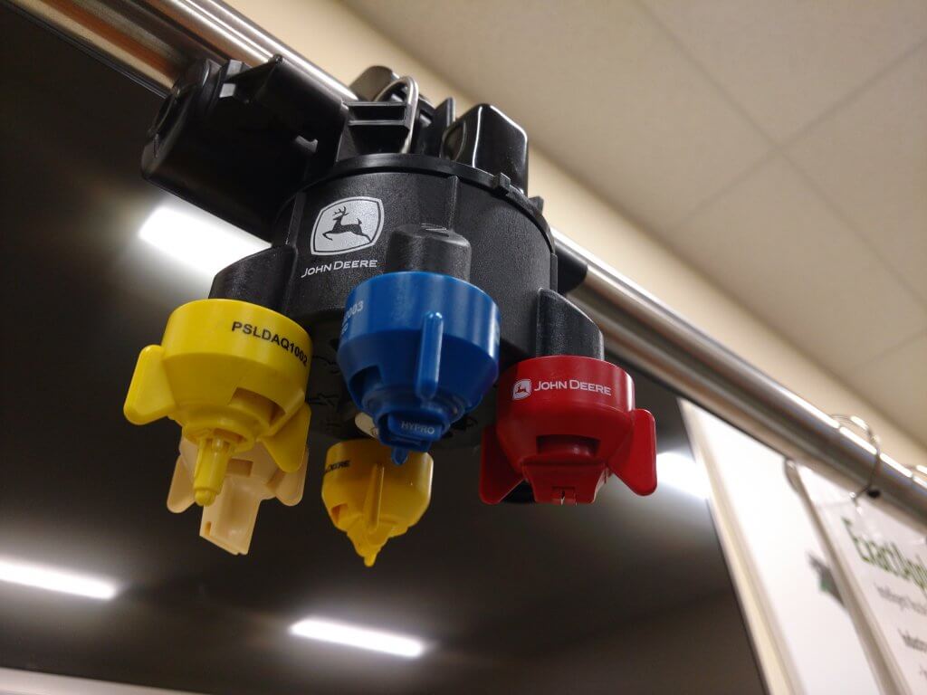
    In early 2021, John Deere announced its entry into the Green on Brown space with See & Spray Select™. This system is built around the ExactApply nozzle body and uses RGB cameras to differentiate green plants from non-green background colours. It will be in fields in 2022 according to John Deere. Similar RGB-based systems are in development by other manufacturers. Although their performance has not been compared side by side with WEEDit or WeedSeeker, initial specs suggest that the RGB systems are slower and are less able to detect small plants. Nonetheless, the future looks very promising.

    In 2021, Hardi Australia announced a new product, called GeoSelect. This system does not have boom-mounted sensors, and instead sprays according to a prescription map developed by a drone. The advantage of this system is that the amount of herbicide needed is known in advance of spraying, and the knowledge of weed distribution in the field can allow for a more efficient coverage plan to be used. This system allows for spraying under any light condition, and adjusts for boom sway to ensure accurate placement. Drone map development is the responsibility of the applicator.

    Green on Green

    Green on Green spraying, which detects weeds within a crop and differentiates them from that crop, is advancing and the earliest commercial releases are now available in Australia, offered by a partnership between Bilberry and Agrifac (WeedSmart podcast here), as well as Bilberry and Goldacres with Swarmfarm. Others, notably the SmartSprayer from Amazone in partnership with Xarvio and Bosch and Greeneye Technology are entering field testing with commercial sized units in 2021 and 2022, respectively.

    Opportunities for Optical Spot Spraying

    Taken as a whole, optical spot spraying offers a number of opportunities for weed management.

    Cost Savings: OSS has an appealing rate of return on investment. On a 5000 acre farm, a pre-seed treatment of glyphosate plus tank mix for resistance management may cost $10/acre, or $50,000 per year. At an average savings of 75%, that represents $37,500 per year. Add other non-crop uses, such as post-harvest, and savings increase. With eventual weed recognition in-crop, virtually all herbicide treatments are candidates for such savings.

    Herbicide Resistance Management: Delaying the onset of herbicide resistance requires the use of multiple effective modes of action in a tank mix. Cost is a deterrent to this practice. With OSS, these tank mixes become affordable.

    Efficiency: With 75% product savings, a tank of product will last longer. The time lost to hauling water and product, as well as filling the sprayer, will decrease. For example, WEEDit users are spraying a full day on a single load. Or they may choose to use a much smaller load, decreasing equipment weight.

    Pre- and Post-Harvest: Whether for desiccation or weed control, site-specificity of late season sprays can also be based on living tissue. Only regions in the field requiring the desiccant are treated. Perennial or late-season weeds are selectively controlled pre-harvest. Since herbicide rates in these applications are typically higher, savings are significant.

    High value crops: Row crops requiring multiple fungicide applications per season, such as potatoes, can benefit from OSS. Sprays applied prior to canopy closure can thus avoid gaps between plants, saving product.

    Producer Innovation: One user of the WEEDit system in Saskatchewan developed an innovative use. Having missed a pre-seed spray, the applicator was faced with large weeds in a 1-leaf RoundupReady canola crop. By turning down the sensitivity of the system so the canola crop did not trigger the sensors and turning on Dual Mode, he was able to broadcast spray the field at a low glyphosate dose (sufficient to control the small weeds) and then apply a full dose to the larger weeds, triggered by the sensor.

    Equipment Innovation: Since individual zones or weeds require unique doses or products, technologies like direct injection, remote nozzle switching, multiple smaller tanks and booms, and PWM will make more sense and grow. But the whole concept of detection and treatment can be moved away from pesticides to mechanical control or other techniques such as lasers, as does Carbon Robotics.

    License to Farm: OSS makes intuitive sense not only to applicators, but also to the public at large. Showing and using these technologies demonstrates stewardship practices that are easy to communicate and understand.

    Artificial Intelligence Scouting

    Another approach is pioneered by several companies, for example Dronewerkers in the Netherlands (https://www.dronewerkers.nl/english/) Taranis (http://www.taranis.ag/), and Xarvio (https://www.xarvio.com). These companies have developed plant recognition algorithms that are currently able to identify over 100 different species. Each species can be divided into several growth stages. Taranis has launched a business in North America that scouts fields by high-resolution drone imagery, and then provides customers with maps that highlight potential agronomic issues such as weeds, disease, or insect damage.

    Example of information available from artificial intelligence scouting. In this case, plant and foreign material information by species, relative abundance, and growth stage.

    Resolution of the output can be species-specific (lambsquarters vs redroot pigweed), or by coarser resolution (broadleaf vs grass). The resulting output then shows the plant density at each location.

    Weeds in a soybean crop (courtesy of Taranis)

    Xarvio Scouting is a product in their Field Manager line (https://www.xarvio.com/en-CA/Scouting). App-based, the agronomist or producer takes pictures of their crops and the app is able to recognize weeds, diseases, insect feeding damage, as well as nitrogen status. The app is aware of other users in the area and basically crowd-sources emerging agronomic issues as they arise, communicating them back to the user.

    The Xarvio Scouting app can identify certain weeds, diseases, and insect feeding damage from pictures taken while scouting (Screenshot from Xarvio.com).

    The agronomic value of this information is clearly very high. Imagine knowing the distribution of weeds by species before and after treatment. Although we can already assess this when we walk fields, by conducting the task via drone we are measuring on a wide scale, permitting an accurate quantification of the treatment effect so its value can be assessed. This level of measurement intensity was not possible before. Yield loss models for time of removal of certain weeds at certain growth stages can be applied across the entire field, and economic analyses allows follow-up treatments to be tailored to specific portions of the field.

    Green-Eye Technology artificial intelligence can differentiate these ragweed plants from the pea crop. (Courtesy Green Eye Technology).

    Or imagine following specific patches of weeds over time, to monitor the effectiveness of a certain cultural practice, or be alerted to the establishment of a resistant population while it’s still feasible to contain it.

    Heat maps can be generated to document weed patches, and perhaps monitor their size over time. (Courtesy Green Eye Technology).

    When this information is converted to a prescription map, rate and tank mix composition (or cultural controls) could be varied as necessary by zone, or weeds could, in the future, be sprayed individually. Perhaps future autonomous robots could be deployed more efficiently.

    Identification of plant symptoms in canola (Courtesy of Taranis)

    Development and improvement of these technologies is ongoing rapidly. Finally, we may have all the pieces that can bring site specific weed, disease, and insect management to market.

  • Ten Tips for Spraying in the Wind

    Ten Tips for Spraying in the Wind

    Choosing the right time to spray can be tricky. Our gut tells us that spraying when it’s windy is wrong.  The experts tell us that spraying when it’s calm is wrong. So when can you actually spray?

    I’ve always advised my clients to spray in some wind, because it has a few advantages. The main one is that wind helps disperse the spray upward and downward, diluting the spray cloud fairly rapidly. Another advantage is that winds tend to be reasonably steady in their direction and velocity (or at least that can be forecast), so downwind areas can be identified and potential impacts are known or predictable. It helps if it’s sunny, because that improves the dispersion of the cloud even more.

    First, let’s define “windy”. The classic wind scale is the Beaufort Scale, intended for the sea, but also used on land. The upper limit for spraying is probably Force 3 or Force 4, with upper limits of 20 – 25 km/h or so.  The Beaufort Scale calls these “Gentle or Moderate Breezes” (they had to save the alarming words for hurricanes), and the scale provides good visual clues such as what wind does to flags, leaves, or dust.

    Beaufort Scale-1

    Spraying under breezy conditions can be done fairly safely if you follow specific steps. The idea is to understand what the risks are and to manage them.

    The cornerstone is to use a low-drift spray and match it to a pesticide that will work well with larger droplets. But there are other important aspects to consider. Below are the top ten to think about:

    • Choose a herbicide that can handle large droplets. Glyphosate products are well suited to coarse droplets. But glyphosate commonly has contact actives in the mix, members of Group 6, 14, and 15, and these are less likely to perform well with big droplets than those that contain Group 2 and 4 mixes. Actives with soil activity also have more tolerance for larger droplets.
    • Use a low-drift nozzle and operate it so it produces a Coarse (C) to Very Coarse (VC) spray quality, as described by the manufacturer. Dicamba labels call for Extremely Coarse (XC) to Ultra-Coarse (UC) sprays, and Enlist requires at least Coarse. To achieve these you may need to purchase new nozzles. Low-pressure air-induced nozzles operated at about 50 – 60 psi will generally be very low-drift, but lower drift models are available. If you need a finer spray, produce it either by increasing the pressure or moving to a finer tip. Do this when the weather improves, for contact modes of action.
    The name, symbol and range of droplet sizes used to describe the median droplet diameter produced by nozzles according to ASABE S572.3
    • Keep your boom low. Lowering the boom ranks as the second-most effective way to reduce drift, after coarser sprays. But there’s a limit. For low-drift sprays, you need at least 100% overlap (more for PWM), which is for the edge of one nozzle pattern to spray into the centre of the adjacent pattern. In other words, the spray pattern should be twice as wide as your nozzle spacing at target height.  For most nozzles, a boom height of close to 20 inches is enough to achieve this overlap. That’s pretty low by current standards from suspended booms on self-propelled sprayers, so being too low for a good pattern will only happen due to boom sway.
    • Maintain reasonably slow travel speeds. These reduce the amount of fine droplets that hang behind the spray boom, reduce turbulence from sprayer wheels, and they also make low booms more practical. An added bonus is less dust generation.
    • Know what’s downwind and what harms it. Survey the fields on all sides of the parcel you’re treating. When you have a choice, avoid spraying fields that have sensitive areas downwind such as water, shelterbelts, pastures, people, etc. If you can’t avoid being upwind of these areas, make sure you check and obey the buffer zone restrictions on the label. These will also give you an idea if the product can cause harm in water or on land, or both.
    • Consider a dicamba tip for special situations, even if you don’t use dicamba. If you’re in a situation where quitting and waiting is a poor option, these tips allow you to finish the job with minimal drift risk and with only slight reductions in product performance due to poor coverage.
    • Use a low-drift adjuvant. Specific products such as Interlock or Valid have been shown to reduce driftable fines (<150 microns) by between 40 – 60%, without adding significant volume in coarser droplets. The response will depend on the nozzle and the tank mix, but can be very noticeable.
    • Study drift and how it forms and moves. It’s about more than wind speed and droplet size. Knowledge in this area can help you work out the best strategies.
    • Invest in productivity. You may not need it every day, but on occasions when you have a small window to avoid bad weather, it pays dividends.
    • If you feel that drift is unavoidable and someone might be impacted by it, talk to those people first. It’s one of the most important things you can do.

    Keeping pesticide sprays on target continues to be one of our top responsibilities.

  • Fundamentals of Spray Drift

    Fundamentals of Spray Drift

    The year 1989 marked my first spray drift trial under the watchful eye of Dr. Raj Grover and John Maybank. We evaluated the performance of several spray shrouds, Flexi-Coil, AgShield, Brandt, and Rogers, and wanted to measure just how effective they were. But in my heart I wasn’t interested in drift. I wanted to study herbicide efficacy. Anyway, I thought, we’ll do this trial and I’m pretty sure we won’t have to revisit the topic.

    It’s now thirty-two years later and spray drift has interwoven itself into all my projects, remains one of the most powerful drivers of regulatory activity, is likely the most visible consequence of poor stewardship, and will stay as one of the dominant creators of public opinion around modern agricultural practice.

    Drift has not gone away. And yet our understanding of it is far from complete.

    Spray drift is defined as the wind-induced movement of the spray cloud away from the treated swath. Droplet drift can occur for all sprays, and it happens within minutes of the spray pass. Its cousin, vapour drift, is limited to active ingredients that are volatile, that is, they can evaporate from dry deposits after application. Vapour drift happens after the spray application is complete and can last several days.

    Droplet Drift

    Droplet drift can be divided into two phases that are separated by about 1 second and that are measured differently. “Initial drift” happens first and refers to the product that leaves the treated area immediately after atomization. It is airborne and can be measured by placing air-samplers (any device that can capture droplets in air) close to the downwind edge of the spray swath.

    Figure 1: Initial vs Secondary drift. Once the drift cloud leaves the treated swath, the relative strengths of turbulence and sedimentation determine the amount that remains airborne and the amount that lands downwind.

    Secondary drift describes the airborne spray cloud that continues to move downwind from the swath edge, where it either remains aloft or deposits on the surface below it. It is typically measured using samplers placed on the ground that capture sedimenting spray droplets. The difference in method is important because it goes to the heart of the problem of understanding spray drift.

    Figure 2: Droplet drift occurs when displacement energy exceeds droplet energy. The droplet’s combination of mass and velocity cannot withstand the energy presented by moving air.

    Initial drift is actually quite easy to understand because its creation is intuitive. The displacement of droplets from the spray plume is a function of balancing two types of energy. The first, droplet energy, is the product of droplet diameter and velocity. The more energy in the droplets, the more difficult they are to displace, and that’s why larger, heavier droplets or fast-moving air assist are useful drift reducing tools.  The second, displacement energy, comes from relative air movement, either from forward travel speed or wind and the associated turbulence. More wind or turbulence means more power to displace.

     Figure 3: Initial drift follows an expected response to greater wind speeds and coarser sprays. Data from a pull-type sprayer travelling 13 km/h with 60 cm boom height.

    Because initial drift is easier to understand, our most common advice for reducing drift is based on maximizing droplet energy and minimizing displacement energy. Lower booms, larger droplets, slower travel speeds, shrouds, or properly implemented air assist all help reduce initial drift. It makes sense that creating less initial drift will also reduce downwind deposition arising from secondary drift.

    Figure 4: Management of initial drift is intuitive. We reduce drift by adding energy to the droplet and by protecting the droplet from exposure to moving air.

    Downwind Deposition

    After leaving the spray swath, the moving secondary drift cloud has two main options. It can deposit or it can remain airborne. Basic physics suggest that all objects eventually fall to the ground, and since smaller objects need more time, they drift further. But when atmospheric turbulence and topography are considered, it’s not quite that simple. These two complicating factors control what proportion of the drift cloud remains airborne, and what proportion deposits.

    Drift trials show that about 20% of the initial drift amount returns to the surface within the first 100 m or so of the sprayer. The rest remains and rises in the atmosphere where it evaporates and gets mixed further.

    Figure 5: The majority of secondary drift remains airborne. Data are for Medium spray quality from a pull-type sprayer with 60 cm boom height and 13 km/h travel speed

    It happens quickly. Just 5 m downwind of the spray swath, the cloud is already 4 m tall. At 100 m downwind, we’ve measured its height to be 30 m.

    The proportion of the spray that remains airborne depends on the spray quality and the nature of the atmosphere. If it’s windy and sunny, or if the spray is finer, turbulence sends more into the air. If it’s cloudy and the wind is low, we have little atmospheric mixing. As a result, a smaller proportion will remain airborne and more will sediment, and overall, we may actually have more potential to damage downwind areas.

    When we graph spray drift deposit data from a windy day, the deposit amount decreases exponentially with downwind distance. Usually, drift damage follows the same pattern. The larger droplets that contain the majority of the dose deposit first. The smaller droplets go further and are more likely to mix in the atmosphere and rise with thermals.

    Figure 6: Deposited drift decreases logarithmically with distance. Top, linear axes. Bottom, log axes.

    Under temperature inversion conditions that are common on calm summer evenings, overnight, and early mornings, the damage from the drift cloud does not decrease the same way. The cloud containing the buoyant mist lingers over a large area. Without atmospheric mixing and its resulting dilution with time and distance, large areas can be damaged.

    The Effect of Turbulence on Deposition

    We’ve established that the more atmospheric mixing we have, the less spray will deposit on the ground, at least in the short term. How does this affect our thinking on the role of wind?

    When we evaluated drift data from a number of trials, we always saw more initial drift with higher wind speeds, as expected. However, the downwind deposit did not usually increase significantly. We attributed this observation to turbulence generated by wind which lifted more of the initial drift higher into the atmosphere. To be clear, deposited drift did not go down with higher wind. It just didn’t rise as fast as initial drift.

    Figure 7: The effect of wind speed on airborne drift (top line) vs deposited drift (bottom line) from a high clearance sprayer travelling 23 km/h and emitting a Very Coarse spray.

    The effect of turbulence can be viewed as a good thing because it protects downwind objects. Rapid dilution reduces immediate drift damage. We can use turbulence to protect objects on the ground. It’s certainly better than the alternative, emitting sprays when the atmosphere can’t dilute them, such as in an inversion. In that case, downwind areas remain at risk for a long distance, and for a long time.

    But we have to also consider what happens to airborne spray droplets. Some pesticides degrade in sunlight and stop being a problem. But others are more stable and may persist in the atmosphere for days or longer. During that time, they may move significant distances, ultimately returning to the earth’s surface in precipitation or in dust. Even though the atmosphere has diluted them, these deposits are measurable, and will show up in environmental monitoring of air, soil, and water.  We may not be able to find out where they originate, but the public knows who to blame. Agriculture.

    Vapour Drift

    Vapour drift is another issue altogether. It occurs hours and days after application, as long as the volatile product remains on a surface and conditions that allow formation of vapours persist. Vapour pressure is related to surface temperature, and losses increase with warmer surfaces. Some products enter the vapour phase when in contact with water, and release vapour after a rainfall.

    In situations where vapour is released for several days after application, it becomes impossible to control its subsequent movement. For droplet drift, if we know the wind direction at the time of spraying, we know where the impact is likely to be. But vapour movement depends on conditions that may occur between now and three days from now, and these could include high temperatures, various wind directions, and even inversions in which vapours accumulate. Ultimately, the best way to avoid off-target vapour movement is to avoid using volatile products.

    The Public Good

    Spray drift is one of agriculture’s most important stewardship challenges, and our industry needs to continue to improve its track record. Sprayers have a difficult task of converting a relatively small volume of liquid into a spray that offers good target coverage yet doesn’t move off the treated area. Favourable weather combined with droplet size management are at the heart of making this system work, but there isn’t a lot of wiggle room. Once again, an emphasis on sprayer productivity is one of the most fruitful areas to invest in, as this makes the best of the sometimes rare conditions in which spraying conditions are optimal.