This article is based on a presentation by Dr. Melanie Filotas, who delivered it as part of the 2019 agriculture summer student orientation day.
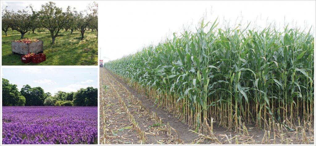
Most crops are sprayed with organic or synthetic pesticides at some point during the growing season. Use caution before entering any area where crops are grown (e.g. corn field, nursery, greenhouse, orchard etc.). Always confirm that it is safe to enter.
Most crops receive some form of chemical input during growth. Be aware of what has been applied.
Even organic operations apply controlled products that may make it unsafe to enter for a period of time.
You can be exposed to pesticides if you enter a treated area before pesticide residues break down and vapours dissipate. The minimal time that must elapse before being permitted to enter is called the Restricted Entry or Re-entry Interval (REI).
REIs are data-driven and established by the federal government. They are defined as: “The period of time that agricultural workers, or anyone else, must not do hand labour in treated areas after a pesticide has been applied.” Hand labour can be any task involving substantial contact with treated plants, plant parts or soil, including planting, harvesting, pruning, and scouting.
Things you should know about REIs:
REIs can range from one hour to several days
If a pesticide label does not indicate a REI, the default is 12 hours
REIs can vary with the product, crop and type of activity (e.g., scouting, harvesting, etc.)
REIs can change over time so always refer to the most recent label
If a tank mix (multiple products) was applied, observe the most restrictive REI
Before visiting an operation to work in the field:
Tell your supervisor where you will be that day
Ask the grower or spray applicator what was sprayed. Records may be posted, but verbal confirmation is preferred
Look up the REI for the product on the crop you will be entering
Check with your supervisor on any products with special instructions beyond the REI
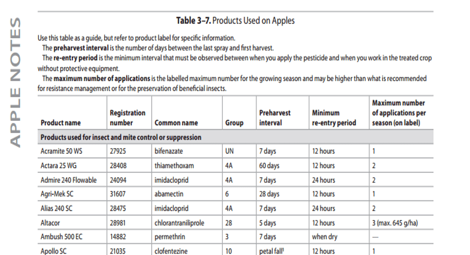
Do not enter the field until the REI has ended. Pesticide REIs can be found in local production guides, or on pesticide labels.
Local production guides summarize REIs.Local production guides list REIs by crop, by product applied, and by activity.
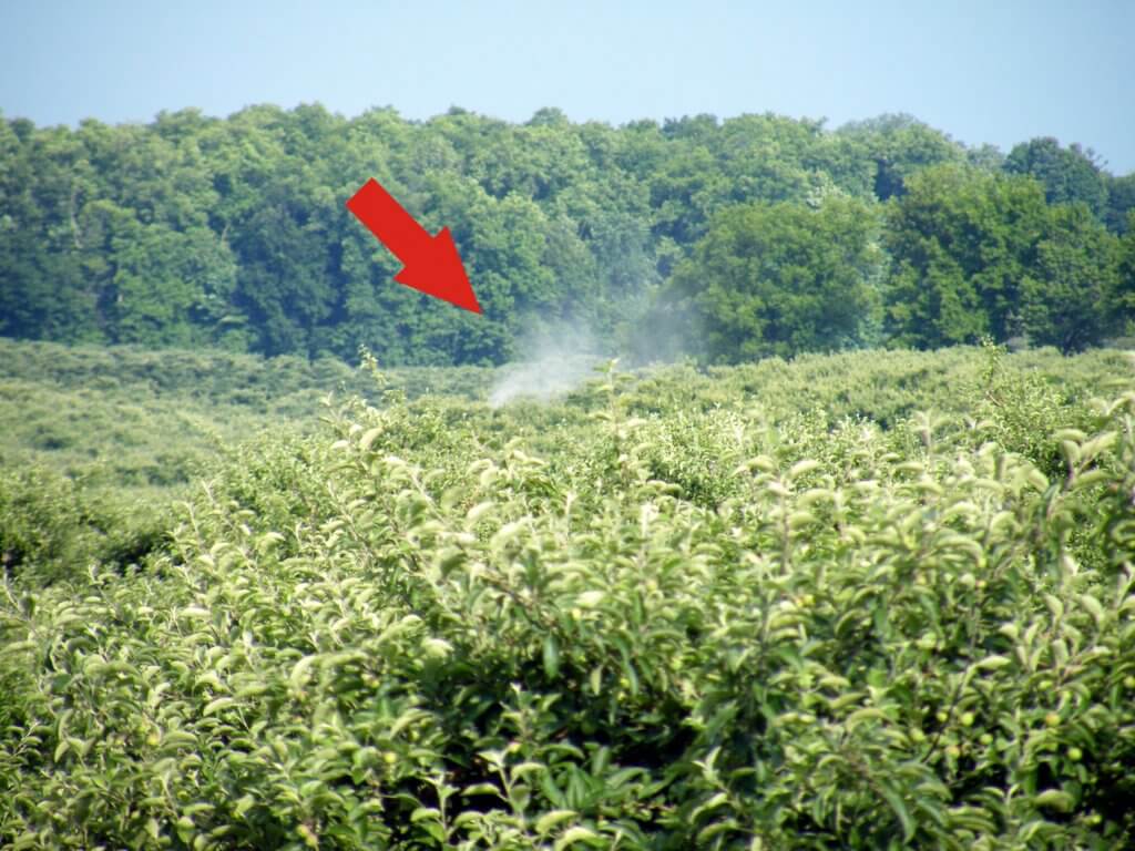
Miscommunication can sometimes happen. Learn to recognize the signs of spraying. When in doubt, leave the planted area and call the grower to confirm or call your supervisor.
In some cases you can look for fresh tracks in the operation, but be aware they may not have been made by a sprayer
Some products have a distinctive odour
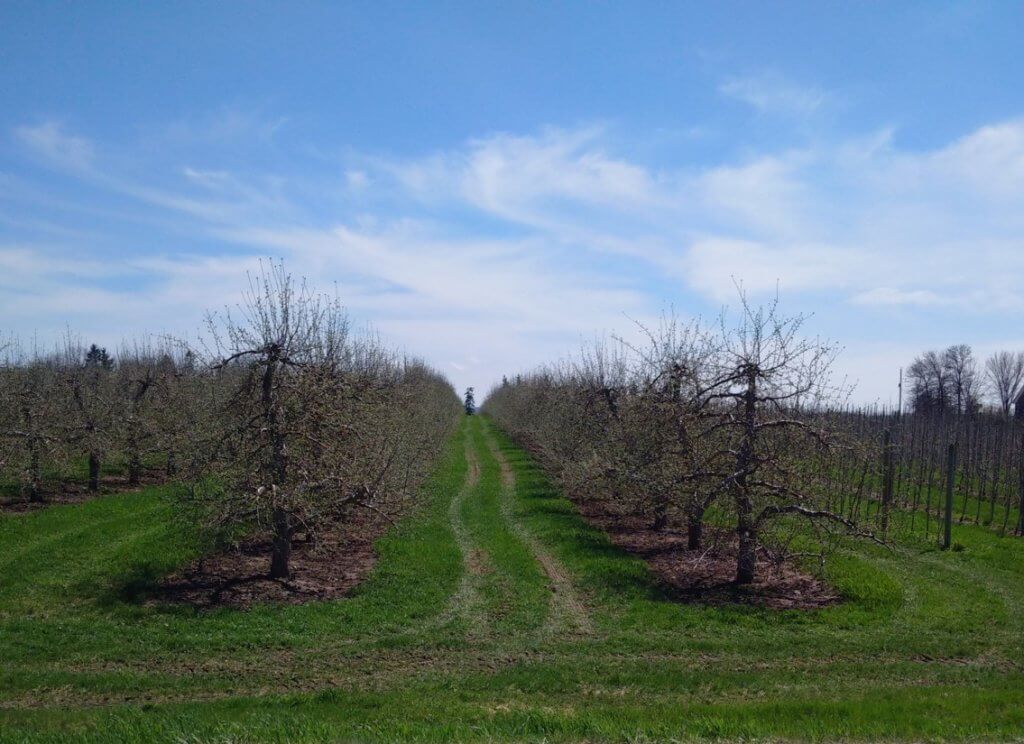
It can be difficult to see a sprayer operating, particularly in orchards, but they can be heard. Do not wear earbuds or headsets while in a production area
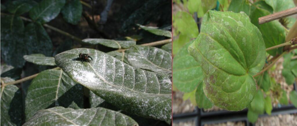
Look for foliar residue. This is an indicator, but does not always mean it is unsafe to enter
Fresh wheel tracks may indicate recent spraying.
Some products have a distinctive odour.
It may be difficult to see a sprayer operating in the vicinity, such as in this orchard. However, they can often be heard. Do not wear a headset or earbuds in a production area.Residue on leaves may indicate a recent application, as in the left photo. However, it could also be unrelated. On the right is calcium magnesium precipitation from irrigation water. (Photo credit [right]: Jennifer Llewellyn)
There are many potential symptoms of pesticide exposure: headache, fatigue, irritation of the skin, eyes, nose or throat, loss of appetite, dizziness, nausea or vomiting, diarrhea, decreased muscle coordination, and blurred vision. Each product has a Material Safety Data Sheet (MSDS) that will provide details on exposure symptoms and treatments.
While sometimes confused with symptoms arising from sun stroke or dehydration, if you suspect pesticide exposure it is always best to be prudent and get medical help immediately. Contact your local poison centre or 911.
Summer work in crop production can be rewarding and enjoyable, but always use caution and be safe.
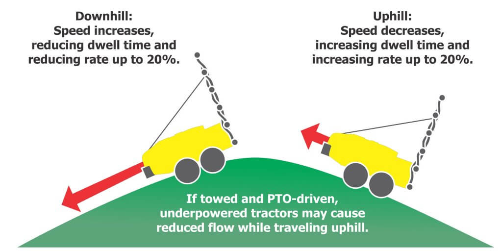
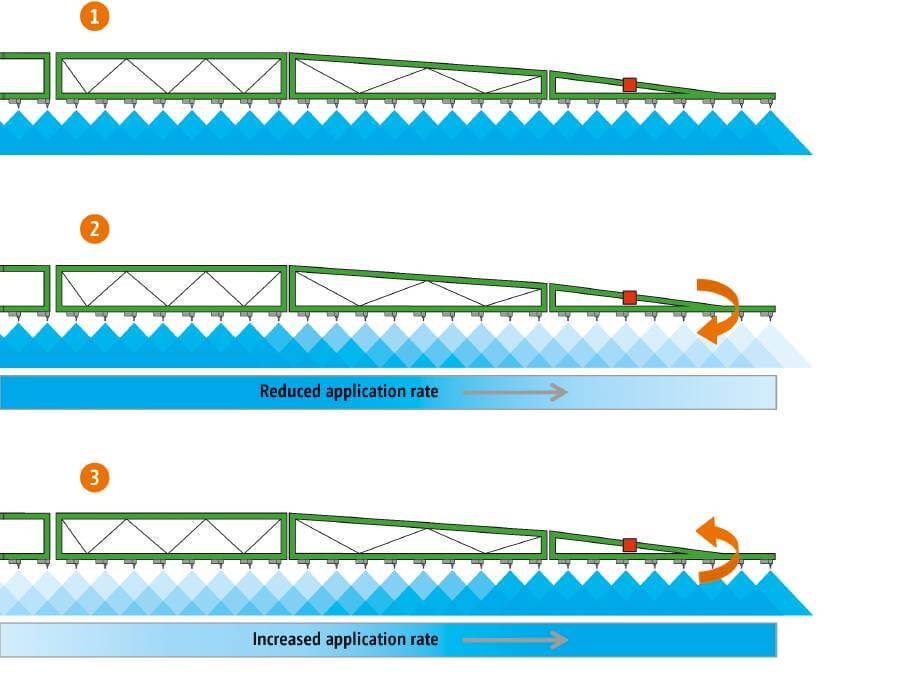
There are many advantages to using rate controllers, but their primary role is to maintain a constant application rate. All sprayers change speed on hills, at row-ends, or in response to surface conditions. Since flow from an uncontrolled sprayer is constant, the application rate varies significantly (up to 40% in hilly conditions). Rate controllers compensate for changing speed by adjusting flow.
Hilly operations create highly variable application rates. Changes in travel speed can translate to 40% variability in rate applied. Rate controllers adjust flow to compensate.
Pesticide is not saved directly (since increased uphill rates already cancel out reduced downhill rates), but consider the pesticide label. Labels that list a range of rates are contingent on pest pressure and crop size, but also compensate for poor coverage from low-performing equipment. When coverage uniformity is improved, experience has shown that operators can safely spray at minimal rates.
Experience has also demonstrated that when coverage uniformity is improved, pack-out benefits follow. Even a modest improvement represents a quick return on investment. Equally important, a more consistent application reduces the risk of higher residue levels on the uphill and improves crop protection on the downhill.
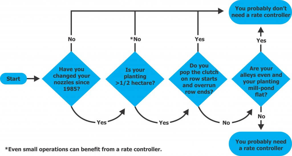
Now, if you are wondering if a rate controller is right for your operation, or if you should just stop reading now, consult this handy decision support matrix:
This decision support matrix will help you decide if a rate controller is right for your operation. Spoiler alert: It probably is.
Rate controller categories
The following table categorizes controllers based on how they control flow. The categories are successively more expensive and complicated, but there’s commensurate value. For example, while not specified here, high-end rate controllers offer value-added features such as as-applied mapping (a powerful management tool).
Description
Pros
Cons
Good: Monitors and adjusts pressure. Uses math to assume flow.
System monitors pressure, but does not register flow. For example, if nozzle flow is restricted, back pressure increases. The controller will compensate to correct pressure, implicitly reducing flow, but the operator is not alerted to the actual problem.
Better: Monitors and adjusts flow, not pressure.
Alerts operator to changes in flow. Operator usually sets the percent error threshold a little high to ignore transient changes.
System will not register pressure deviations. At threshold speed, pressure may drop too low. This can cause inconsistent check valve operation and spray pattern collapse. With tall booms, the top nozzles may close completely.
Best: Monitors flow and pressure and adjusts flow.
-Best likelihood of a consistent application. -Alarms or automatic compensation of flow and pressure (user sets hard stops). -Provides a low tank level warning. -Stores preset calibrations to quickly switch between blocks.
-Highest cost. -Steepest learning curve. -More “wire-wiggling”. -Operators often choose to over-apply at low speeds as a tradeoff for uniform output and consistent atomizer performance.
Rate controller adoption and components
As we write this, less than 10% of air-assist sprayers have rate controllers. In the dark old days of the 1980’s, air-assist operators were ill-advised to install high flow, low pressure field sprayer controllers. That history of mismatched components and subsequent bad experiences continues to hinder widespread adoption.
Today’s components, however, are specific to air-assist sprayers and have made installations easier and more successful. Do your homework and speak with the manufacturer (not necessarily the local dealer) to ensure the controller, and all its components, meet your needs. Let’s describe the components so you’re prepared to have the conversation:
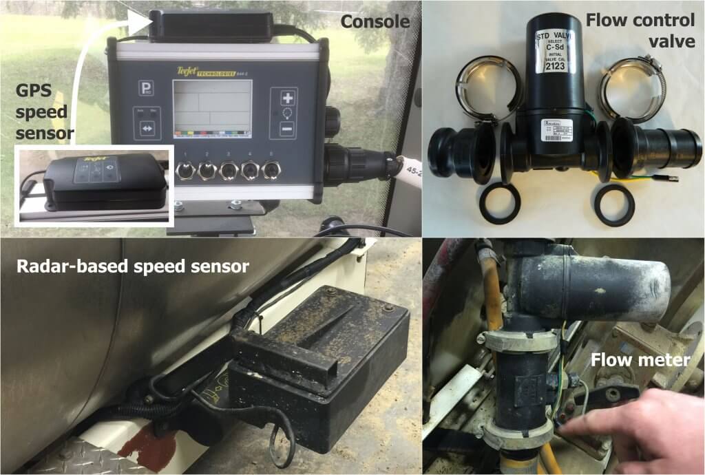
Console
Flow meter(s)
Flow control valve (including electric boom shut-offs)
Speed sensor
Wire harness
Examples of rate controller components.
Console
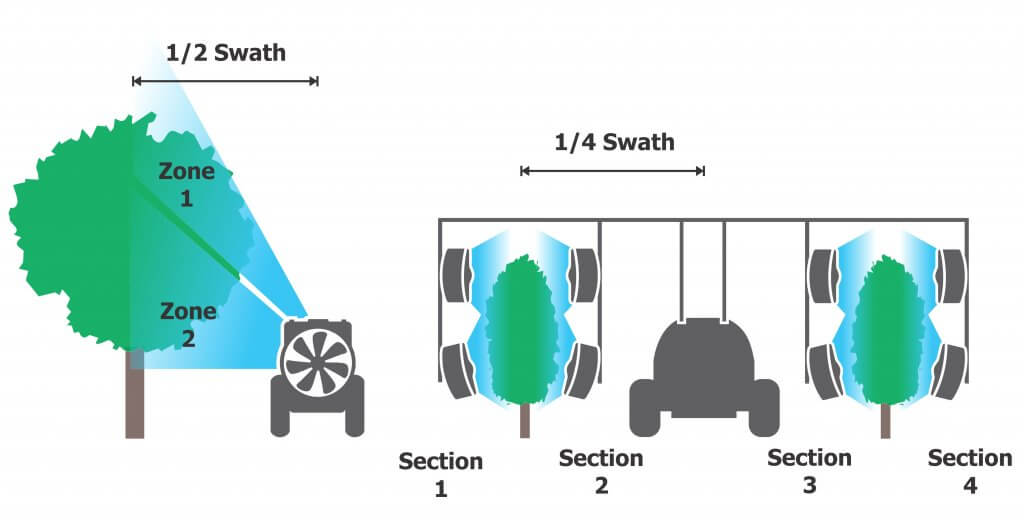
The console is the interface. The user enters criteria about the sprayer, the planting, and calibration data and receives information about sprayer performance. Select a console designed for air-assist sprayers and not field sprayers. Controllers intended for horizontal booms perceive swath in two dimensions, but air-assist controllers account for multiple vertical booms or boom sections in the swath (see the following figure).
Field sprayer rate controllers used in vertical crops must be “tricked” when programming swath. Leading air-assist rate controllers can assign flow to zones on a single vertical section (left) and adjust swath (sometimes called width) for multiple booms (right).
Flow meter
With rate controllers, flow is detected by one or more flow meters positioned pre-manifold. The relief valve becomes more of a safety device, defining the high pressure limit and bypassing flow if required. Most rate controllers use a flowmeter with no ability to monitor pressure. While still effective, adding a pressure sensor ensures nozzles are operating in the desired pressure range.
Turbine or paddle meters are inexpensive and acceptably accurate. They require periodic cleaning because some chemistry can accumulate and interfere with their moving parts. Filtration helps to minimize this issue. Magnetic or ultrasonic meters have no moving parts, higher resolution, wider metering ranges and aren’t affected by the viscosity of the spraying solution or entrained foam. However, they are considerably more expensive than mechanical meters.
Flow control valve
Unlike boom control valves that are open or closed, flow control valves are capable of a range of adjustments. Valve actuation is controlled by 12 volt servomotors. The level of precision depends on the style of valve.
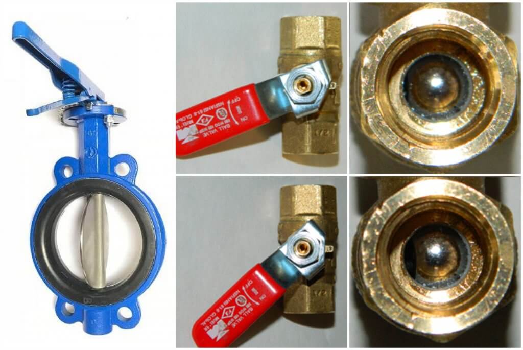
Butterfly valves: Simple, inexpensive, and typically for pressures <10bar (150psi). Some have minor leak-by when closed. Control is less precise as the valve opens because the orifice gets geometrically larger. This gives a narrow metering range.
Calibrated ball valves: Versions available for all pressures. May be simple flow through balls with similar metering limits to a butterfly. A better ball design is also available that offers a linear flow rate through the entire adjustment range, offering more stable rate control over the entire flow range. Several manufacturers offer these. All ball valves offer zero flow when closed.
Left- A butterfly valve. Right- A ball valve. Notice how a small change in the opening angle translates into a large change in the orifice size; this is difficult to control manually. Servomotors not pictured.
Compared to field sprayers, air-assist sprayers travel slower and use lower flow rates. It is a mistake to employ valves intended for high-flow, high-speed sprayers.
Speed: Valves are rated by connection size (½”, ¾”, etc.) and opening time (e.g. 1-14 seconds are common). Many rate controllers can be programmed to optimize adjustments for the speed and size of the valve.
Precision: As control valves open over their 90° range, the ability to control flow is less precise. Slower valves give less precision, but greater stability.
Size: Valve size should accommodate maximum flow and no more. If the valve is too large, it can only meter flow over the first few degrees of opening. For example, let’s say a valve capable of 200 L/min (50 gpm) and rated 1 second is used. Your sprayer meters 0-20 L/min (0-5 gpm). This means the whole metering range happens in the first tenth of a second. Even lightning-fast consoles will give unstable readings (aka hunting) as the computer overshoots the target in an effort to comply.
Control valves are “service parts”. Seals, moving parts and abrasive liquids mean they will require regular care and eventual replacement. It’s a wise precaution to make them accessible and easily removable. We suggest installing them with quick-connects (see top-right of the previous collage of rate controller components above) to make field-maintenance fast and easy.
Speed sensor
Speed can be based on GPS, engine tachometer readings, radar, or wheel rotations. Newer rate controllers may even take the speed directly from the tractor’s data feed. Price, reliability and crop conditions are all factors you should consider in the choice.
GPS: Easiest to deploy, very accurate (especially RTK-GPS) and reasonably priced. However, overhead canopy can block satellite signals. Some controllers compensate for the GPS losses with sophisticated internal kinematic devices that measure the inertia of the sprayer and calculate speed when the GPS is not reliable.
Wheel rotation speed sensors: An entry-level sensor, it’s typically a reed switch or Hall effect sensor that detects either the lug nuts or magnets installed on the rotating wheel. More magnets improve accuracy. Its exposure makes it prone to physical damage, and readings change with tire radius (which changes as the tank empties, on soft ground and with temperature). This is why wheel sensors are calibrated in the alley, with the tank half full and both tires at the same pressure.
Radar speed sensors: Employing the Doppler effect to measure speed, radar is the most accurate sensor. They are unaffected by terrain, slope or tank volume. They can be mounted anywhere in sight of the ground. They are, however, the most expensive and are typically not repairable if they fail.
Tachometer speed sensors: Largely obsolete, they measure the tractor’s tachometer speed and convert it to travel speed. Difficult to install and prone to the same inaccuracy as wheel sensors.
Interface sensors: Relatively new, some rate controllers interface with tractor electronics to receive speed data. ISOBUS, the standard interface language that agricultural electronics are increasingly adopting, makes this data exchange more common.
Wire harness
It may seem we’re drilling deep to mention wires, but standards are changing. Many controllers employ traditional analog wiring, but they are being made obsolete by the newer ISOBUS option.
Traditional Analog: Simple wires with automotive or custom plugs designed to match components. Relatively inexpensive and sometimes field repairable, analog wiring carries signal voltage (and power) to and from the controller to drive valves and receive analog sensor data. Communication is one-way: Sensor to controller, controller to valves.
Modern ISOBUS: Bus systems are more like a computer network, where digital signals travel back and forth between the controller and each component. Components that require power are wired directly to a battery. This results in a greatly simplified harness. The controller’s single ISOBUS wire “daisy chains” all components to relay commands and receive status, which makes system monitoring and diagnosis easier and more effective.
Conclusion
Rate controllers are a worthy consideration for your existing or future air-assist sprayer. Assess your needs and work with a knowledgeable dealer or manufacturer that can assemble and install a system appropriate for your operation.
This short article is a reminder for sprayer operators to respect the possibility of tipping a sprayer. Every spring I catch wind of someone tipping over. When I can ask the operator questions I start with “Is everyone alright?” and “Was the sprayer full?“. Hopefully the answers are “Yes” and No“, but not always.
The following factors are always involved:
Driving too fast. Usually entering a field at road speed.
Entering the field on a downhill slope and/or catching a pothole or soft shoulder.
Turning in a tight radius, usually 180 degrees. This is made worse when the sprayer is towed.
Sprayer is not completely full and “slosh” changes the centre of gravity.
Narrow tires and a narrow base.
Fortunately the sprayer wasn’t damaged and the spill was minor.A tight turn at high speed coupled with a depression in the entryway and tank slosh was enough to tip the unit. They had it righted and hauled out soon after. No one was hurt.
I’ve heard as many cases involving seasoned operators as new operators. The next few pictures are of a veteran operator’s sprayer carrying 28%/ATS. Just like the images above, a tight turn at high speed sloshed the load just as a deep pot hole caught the outside front wheel. This sent the sprayer into a lane of traffic before it tipped back and over into the field. No one was hurt.
Fortunately for the operator, the spill was contained in their field (not the road or ditches). The 90′ boom had to be cut off before the sprayer could be towed back to the yard to be sold off as parts. While the operator has looked at the bright side (an opportunity to upgrade) it has left them relying on a custom operator for spring spraying and making a hasty in-season equipment purchase.
Lost a tire during the tow back to the yard.Crumpled boom after having to be cut from the sprayer.Not the way anyone wants to see their sprayer.
Major Spill
What follows are generic steps for what to do if there is a major spill. Always defer to the process outlined by your regional authority.
If you do tip the sprayer, first protect yourself, then others, then animals in that order.
Stop any exposure by removing clothing and washing as best you can.
Stop people from entering the area.
If it is safe to do so, try to prevent the spill from spreading.
Contact your local spill centre. In Ontario, the Spills Action Centre will receive calls 24 hours a day at 1-800-268-6060. Consult with your municipality for their spill reporting contact numbers.
Take home
Of course we’d rather avoid this problem altogether. Be sure to slow down before turning into a field. Take the turn as gradually as possible. Remember that soft spring ground and new pot holes can become serious obstacles – consider scouting the entry before the first spray or at minimum getting out of the cab and checking before entering.
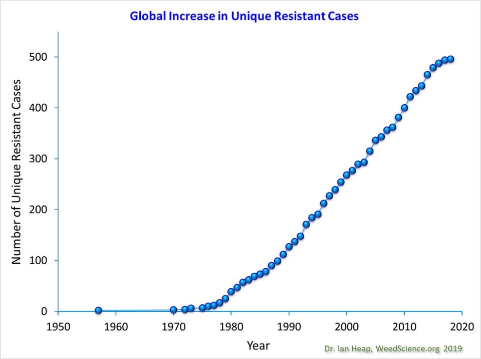
Herbicide resistance has been called the number one threat to conventional herbicide-based weed management strategies.
Since the 1970s, the number of cases of herbicide resistant weeds has shown a linear increase both globally (currently at about 500 documented unique weed species x mode of action cases) and within Canada (at about 70 such cases), according to the herbicide resistance website WeedScience.org. The rate of increase has been constant, and there is not yet any reason to believe that growth in the number of cases will slow.
Figure 1: Growth of global herbicide resistance cases (Source: WeedScience.org)
By using herbicides, we select for weed biotypes that, for some reason, can tolerate the product. Mutations which confer herbicide resistance are rare, but present at very low levels in most weed populations. Repeated use of the same mode of action will increase the relative frequency of the resistant biotype until it becomes noticeable, and shortly thereafter, problematic.
The best-known forms of resistance involve single-gene mutations that alter herbicide target sites (target sites might be enzymes that produce essential plant cell building blocks) so that herbicide binding is reduced, resulting in reduced control. As a result, the target pathway keeps working, and the plant grows normally after herbicide application. Other forms of resistance involve the overproduction of the target enzyme by the plant, mechanisms that either metabolize or sequester the herbicides, or changes in uptake of the herbicide. The main mechanisms are summarized in this table:
Table 1: Mechanisms of herbicide resistance*
Resistant Class
Mechanism
Target Site
Target site mutation
Increased gene copy number
Enzyme over-expression
Non Target-Site
Enhanced metabolism
Differential uptake
Differential redistribution
Sequestration
Delayed germination
Rapid necrosis / defoliation
*Source: Bo AB, Won OJ, Sin HT, Lee JJ, Park KW. 2017. Mechanisms of herbicide resistance in weeds. Korean Journal of Agricultural Science 44:001-015.
The simple act of using a herbicide can select for resistance to that herbicide. While we can’t predict or prevent resistance entirely, we can slow its onset by reducing the frequency of herbicide use, for example by integrating cultural controls such as crop rotation, seeding rate, cultivar competitiveness, and other factors into our agricultural systems.
A powerful option to slow resistance development is to reduce our reliance on a single mode of action, either by rotating modes of action in successive sprays, or, more importantly, by tank mixing multiple effective modes of action (MEMoA) whenever we make an application.
Let’s not kid ourselves. The recent discovery of glyphosate (e.g. Roundup) -resistant wild oats in Australia, and glufosinate (e.g. Liberty) -resistant ryegrasses in several countries is sobering. Relying more on these herbicides will only increase selection pressure.
If we decide to use herbicides, we need to look at the situation from the perspective of delaying the onset of resistance. What we’re trying to do is buy some time, so that new strategies can be developed.
How can spray application methods slow the onset of resistance?
The use of herbicides will continue to select for resistance. The best we can hope to achieve within a herbicide system is to delay that eventuality.
To better understand our options, we need to talk about a specific type of herbicide resistance called polygenic resistance. This refers to accumulation of additive genes of small effect over time, a process that is more efficient in plants that share genetic material among plants in a population, i.e., they outcross.
Outcrossing plants receive genetic material from others, increasing their genetic diversity, and therefore their ability to adapt.
In a field, a population of any specific weed may contain some individuals that have slightly greater tolerance to a herbicide than others. If we apply a slightly lower than label herbicide dose to those individuals, they might survive the application and eventually cross with other survivors and set seed. Their offspring may be as tolerant or even more tolerant than their parents. If this repeats itself over successive generations, the additive effects build until finally, low-level resistance becomes full-blown resistance and even label rate herbicides no longer work. This resistance isn’t a single gene mutation, it’s simply an accumulation of tolerance due to several genes which impact how much of the herbicide active ingredient reaches the target site.
In a recent study at the University of Arkansas, susceptible Palmer amaranth (P. amaranth has both male and female plants and is therefore an obligate outcrosser) was treated with a range of dicamba doses to identify individuals that survived the higher doses. The researchers allowed the survivors to cross, and then grew out their seed, then repeating the procedure. After just three generations, the experiment produced individuals with a three-fold increase in LD50 (compare LD50 at P0 (111) to P3 (309) in Table 2). Recall that LD50 refers to the dose required to observe 50% of the full effect.
Table 2: Dicamba doses (g ae/ha) required for 50% (LD50) and 90% (LD90) control of Palmer amaranth populations selected following sublethal doses of dicamba in the greenhouse.*
Herbicide resistance cannot be prevented if herbicides are applied.
To prevent polygenic resistance, we need to apply the full label rate and avoid repeated sublethal doses, so that all weeds are killed;
We need to apply Multiple Effective Modes of Action (MEMoA) whenever possible so that when one fails, the others have its back;
How can this be achieved?
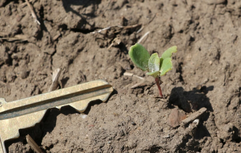
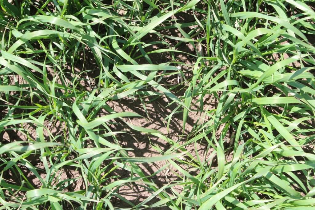
Prevent application practices that result in less effective dosing. Larger weeds, or weeds growing in difficult environmental conditions, may require higher herbicide doses. Early application is helpful because small weeds are easier to control. In addition, crop canopy shading at later staging leads to dose reduction and increases dose variability. Spraying under windy conditions also reduces dose, and can increase deposit variability. For some herbicides such as glyphosate or diquat, the dust generated by wind or fast travel speeds can reduce effectiveness.
Figure 2: Smaller, exposed weeds require lower doses to controlFigure 3: Crop canopies provide valuable competition to help suppress weeds, but they can also intercept spray, reducing the dose received by weeds.
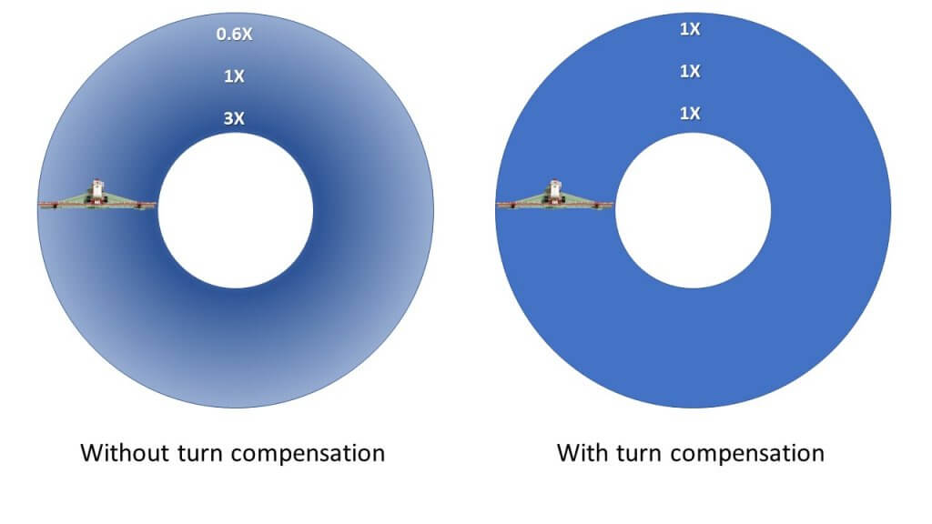
Get Pulse Width Modulation (PWM) with turn compensation. If your sprayer makes the same turn around the same feature year after year, then the outer boom region will under-dose the same part of the field over and over. This is the breeding ground for polygenic resistance. Look for this in field corners, around water bodies or tree bluffs, rock piles, etc.
Figure 4: PWM correction of under-dosing during a turn
Prevent boom sway and yaw. Boom movements result in uneven application, which results in lower control. Pull-type sprayers with supporting wheels are best, but these are becoming rare. Suspended boom performance depends on the manufacturer and the levelling technology they use. However, boom movement is usually more consistent with slower travel speeds.
Figure 5: Boom yaw causing over- and under-application (Source: Farmonline.com.au)
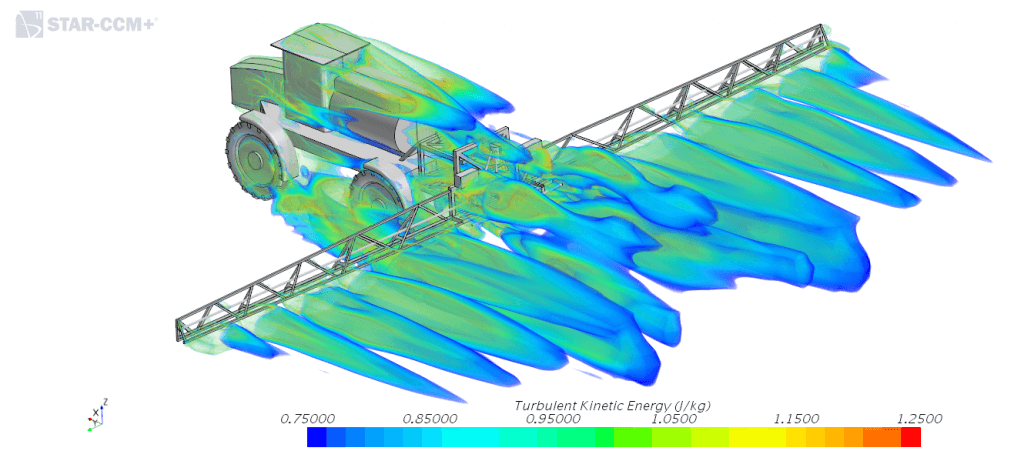
Minimize air turbulence. Large sprayers, and those moving at fast speeds, create aerodynamic turbulence that can displace spray. The main problem spots are wheels, in whose tracks measurably less spray is deposited. The exact dynamics of turbulence is still unknown, but we do know that its magnitude can be reduced with slower travel speeds.
Figure 6: Turbulence due to sprayer speed (Source: Dr. Hubert Landry, PAMI)
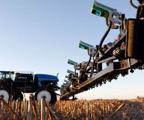
Consider spot spraying. The use of optical spot spray equipment, such as the new WEEDit Quadro, or Trimble’s WeedSeeker II, save product during burnoff or post-harvest. These savings can make the use of more elaborate, expensive tank mixes containing multiple effective modes of action, affordable.
Avoid spray drift. Field margins that harbour weeds rarely receive a full dose of herbicide. Exposing these weeds to spray drift won’t kill them. But it will, over time, select for weeds that are more able to tolerate the herbicide.
Implications
Aside from specific technology such as PWM, improved booms, or a spot sprayer, the most effective fix for variable application doses is slower travel speed.
While this may seem problematic when timing is critical and greater productivity is required, there is a way to drive more slowly and still get more done. We simply need to look at productivity differently.
We tend to equate productivity with speed. Travel speed. But a spray day is filled with many hours of non-spray time – filling, cleaning, transporting, repairing, fueling, record-keeping, etc. How much time is lost to these activities depends on the operation, but for everyone, it’s useful to do time accounting.
Record how a spray day’s time is spent. Pay attention to activities during which you can save time without much expense.
Action
Actual Time
Target Time
Fuelling, lubing
Loading jugs and totes
Checking label (rates, rainfastness…)
Filling tender tanks
Loading sprayer (in yard)
Transport to field
Entering field data into monitor
Checking, recording weather
Checking for pest, stage
Changing nozzles
Spraying load
Unplugging / replacing nozzles
Replacing nozzle body
Making turn
Filling sprayer
Getting sprayer unstuck
Driving to tender truck
Waiting for tender truck
Spraying out tank remainder
Cleaning tank
Cleaning filters
Flushing boom ends
Loading sprayer (in field)
TOTAL
On any given spray day, less time spent filling, or transporting, is credited to spray time. Our analysis shows that time lost to driving slower can more than be made up with these changes. The productivity gain gives more opportunity to spray under more ideal conditions that save yield and also ensure more uniform application.
Using productivity analysis, spraying can become more uniform and help delay the onset of resistance.
Note: The assistance of Dr. Charles Geddes, Research Scientist at AAFC Lethbridge, in drafting this article is appreciated.
In April 2014, NDSU extension published an excellent factsheet explaining what thermal inversions are, how to detect them and how they affect pesticide spray drift. That factsheet inspired this article.
The Atmosphere
The Earth is surrounded by a layer of air called the atmosphere. Think of it as a sheet of liquid percolating and flowing over the Earth’s surface. Seems a bit precarious, doesn’t it?
We define “layers” of atmosphere based on their distance from the Earth’s surface (see image below). We’ll focus on the lowest part of the Earth’s atmosphere: the Surface Boundary Layer. As it drags along the Earth’s surface it experiences rapid changes in wind speed, temperature and humidity (on a time scale of an hour or less).
The Earth’s Atmosphere. The illustration of the Earth is to scale, but obviously the landscape is not. Our focus in on the Surface Boundary Layer.
Atmospheric temperature
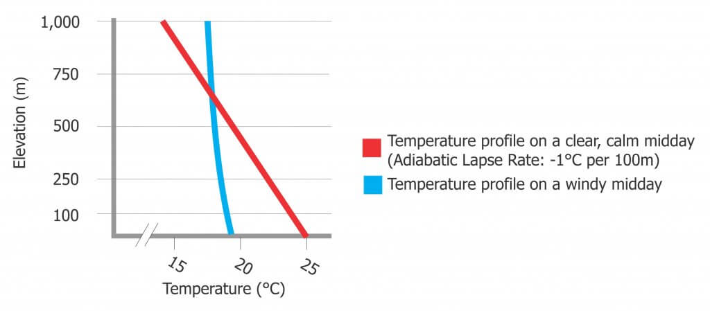
In relatively calm, clear and dry conditions (e.g. a nice afternoon), air cools with elevation at a rate of about 1°C per 100m. This change is called the Adiabatic Lapse Rate and it’s caused by pressure changing with elevation. If your ears have popped when driving down a steep hill, you’ve experienced pressure change with elevation; there is more atmosphere overhead and the weight pushes down.
With higher elevation, there is less atmosphere overhead. Less weight means less pressure and this gives air room to expand. Expansion takes work and work costs energy, which creates a cooling effect. See how simple thermodynamics are?
In the graph below, the red line shows the Adiabatic Lapse Rate of air cooling with elevation. The blue line indicates wind stirring and homogenizing the atmosphere, reducing the degree of temperature change with elevation (more on that later).
Day and night
When we add the effect of daytime solar heating and nighttime cooling, the rate of temperature change is affected. Let’s consider how this works on a clear, relatively calm day:
Early morning
The morning sun emits short wave radiation, which is absorbed by the Earth’s surface. The surface conducts some of this energy deeper into the ground and also heats the air near the surface. This creates a temperature gradient wherein the surface is warmest and the air gets relatively cooler with elevation (remember the red line in the graph above).
As the air near the surface warms, that energy causes air molecules to vibrate and push away from one another. Parcels of air become less dense and rise just like the gloop in a lava lamp. The cooler air around it falls to fill in the space left behind, and air begins to circulate in a Convection Cell. The rising parcel of air will eventually cool and shrink as it rises through the relatively cooler air above it.
These convection cells create Thermal Turbulence, which is a very effective way for airborne particles, such as pesticide vapour, to be rapidly diluted. This is also how the atmosphere disperses pollution. More on the process of dispersion, later.
Mid to late afternoon
As the sun passes over and the wind starts to rise, the convection cells get disrupted by the wind and experience mechanical turbulence (remember the blue line in the graph above). So, mechanical turbulence also mixes warmer air near the ground with cooler air above it, but suppresses thermal turbulence.
Mid-afternoon to night
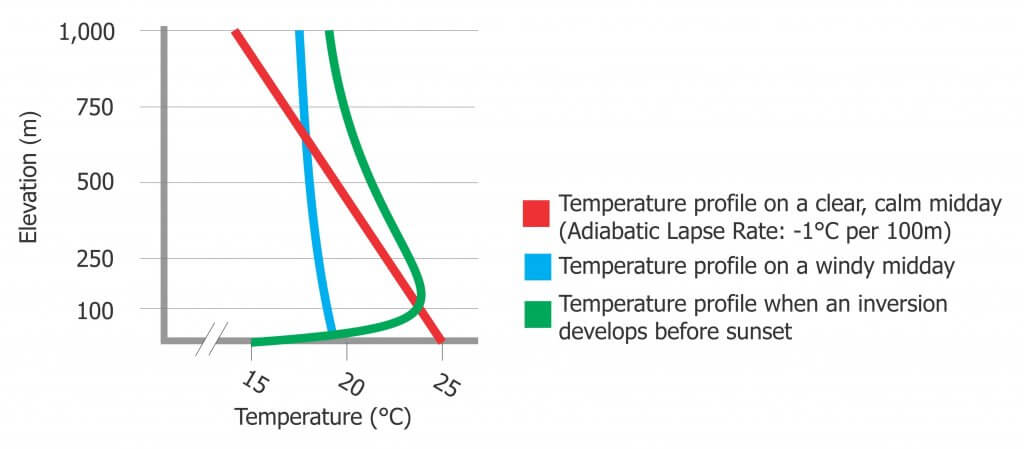
As the energy from the sun lessens, the soil begins to cool and so does the air next to it. Once the air cools enough to be colder than the air above it, we have the beginning of a Radiation Inversion, which is a specific kind of Thermal Inversion (see the green line in the graph below). It is called that because we now have the reverse of the typical day-time temperature profile. The height of the inversion (the ceiling) grows with time, and can reach a maximum of about 100m by sunrise. Within the inversion layer (before the green line bends back at 100m), turbulence is suppressed. We have a stable air mass. More on that below.
How inversions affect dispersion
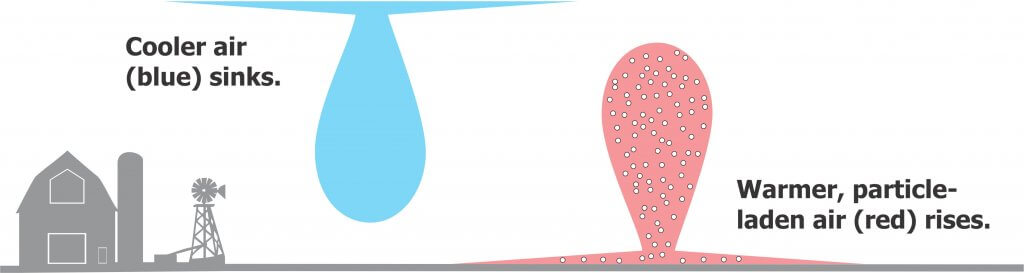
The rising portion of a convection cell carries whatever particles are in the air with it. Suspended particles become much less concentrated at ground level thanks to the thermal turbulence.
Thermal Turbulence allows particle-laden warm air to rise and clean cool air to fall. This disperses air-borne particles like dust or pollution.
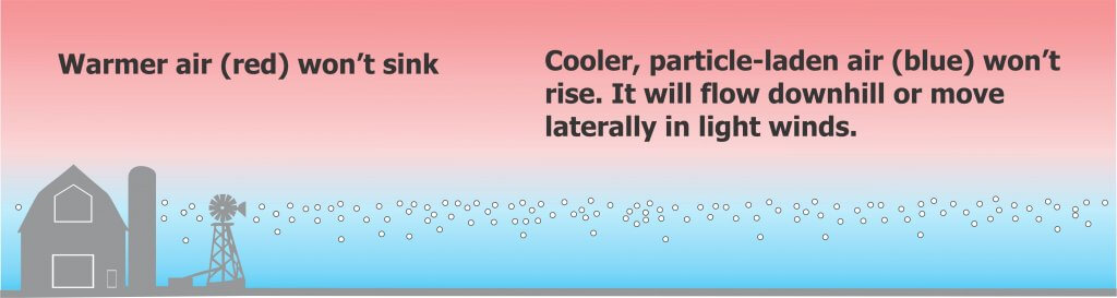
Now let’s imagine we are in a thermal inversion. The cooler, particle laden air near the ground cannot rise and the cleaner air above, which is now relatively warmer, cannot sink. Thermal turbulence is suppressed, and so is any vertical dispersion.
Thermal Turbulence is suppressed during a Temperature Inversion. Particle-laden cool air at the surface cannot rise, and warm, clean air cannot fall. No dispersion occurs, and the concentrated, particle-laden air tends to move downhill or laterally with light winds.
When spraying, the smallest spray droplets fall slowest, staying airborne for long periods of time. If spraying occurs during an inversion, those particles accumulate beneath the inversion layer. Remember we said our atmosphere behaves like a liquid? The colder, denser (pesticide-laden) air drains downhill into low-lying areas. It can also move laterally over great distances, in unpredictable directions, when light winds begin.
Clouds
If the morning were overcast instead of clear, the clouds would intercept much of the sun’s short-wave radiation, absorbing or reflecting it back into space. The Earth’s surface would still warm, but more slowly, suppressing thermal turbulence. As an aside, if clouds form in the evening, they reflect long-wave radiation from the Earth’s surface back down. This Greenhouse Effect is why overcast nights are warmer than clear ones.
Therefore, extended periods of mostly clear skies in the evening or night means a high probability of strong temperature inversions. Conversely, cloud cover usually means a near-neutral atmosphere, so no strong inversion.
Wind
Inversions are only mildly affected by light wind (e.g. 6 to 8 km/h), but as the wind increases and mechanical turbulence mixes the air, the strength of the inversion will be reduced and the atmosphere will approach a neutral condition (see the blue line). In this condition, airborne particles are not dispersed by thermal turbulence, but some mixing will occur. So, there may not be a thermal inversion, but spraying would still be inadvisable if the wind got too high.
Humidity
Inversions form more rapidly when there is less water vapour in the air to absorb radiation. Once humid air has cooled to the dew point, water condensation gives off energy and warms the air a little. This slows the formation of the inversion. Be aware that inversion conditions can exist long before fog, dew or frost forms, so they are not a good indicator for the beginning of an inversion – you’re already in one!
If you see fog, dew or frost, you’re already in an inversion. The air has become cold enough to condense or even freeze water.
Soil conditions and topography
This is a complex issue, but soil conditions that make inversions more intense include low soil moisture, freshly tilled soils, coarse soils, heavy residue and closed crop canopies. Topography matters, too. We’re discussing radiation inversions in arable regions, and the kind that form on mountains or deep valleys. Nevertheless, inversions in shaded areas (e.g., behind windbreaks) start sooner, and last longer. See the NDSU factsheet for more detail.
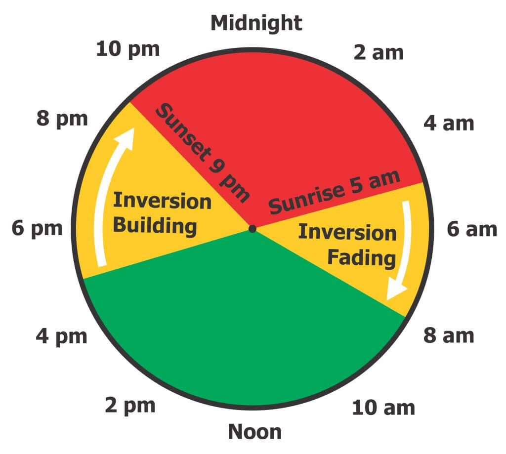
Spray timing
Inversions, once formed, persist until the sun rises and warms the Earth’s surface, or until winds increase and mix the stationary layers of air together, re-establishing a more neutral temperature profile.
Sunset is not a good indicator of the beginning of an inversion – it can start a few hours before. Therefore, evening spraying may be just as risky as night spraying. Very early mornings (e.g. around sunrise) are not much better. Remember, at sunrise, the inversion will be at its maximum height.
The rising sun will warm the earth and create turbulent conditions, starting near its surface (e.g. a few metres). Most inversions will have dissipated two hours after sunrise, which may be the best choice for spraying.
Detecting an inversion
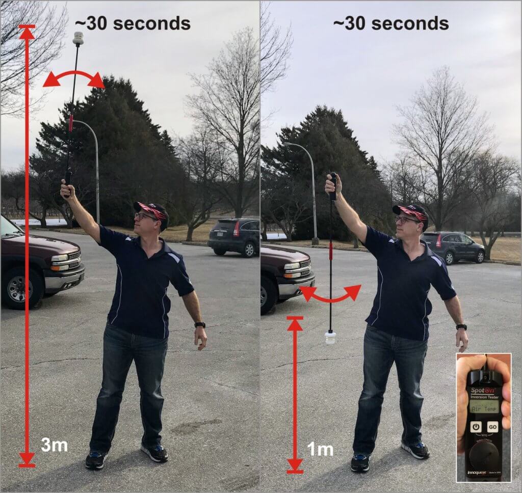
The only sure way to know if you are in an inversion is to take two air temperature readings: one near the ground and one about three metres higher. If the surface air temperature is cooler, you are in an inversion. The magnitude of the difference indicates how strong the inversion is.
Accurate measurements are difficult to manage with conventional thermometers, but SpotOn now makes a hand-held detection unit. If you have one, be sure to let it acclimate before you use it. Leaving it in a hot, or cold, truck or sprayer cab prior to use means it may give a false reading.
Inversion forecasting is getting better, but it’s still location-specific and not entirely reliable. Sprayer operators should learn to watch for the following environmental cues:
Large temperature swings between daytime and the previous night.
Calm (e.g. less than 3 km/h wind) and clear conditions when the sun is low.
Intense high pressure systems (usually associated with clear skies) and low humidity where you intend to spray.
Dew or frost indicating cooler air near the ground (fog may be too late).
Smoke or dust hanging in the air or moving laterally.
Odours travelling large distances and seeming more intense.
Daytime cumulus clouds collapse toward the evening.
Overnight cloud cover is 25% or less.
Note: If you suspect a temperature inversion, don’t spray.
For more information on how weather affects drift, download this pamphlet from the Australian Government Bureau of Meteorology.