Theodor Leeb started building self-propelled sprayers in Bavaria, Germany in 2001 and formed a partnership with Horsch LLC in 2011 (Horsch has been selling tillage and seeding equipment in North America since 2001 and has 17 dealers in the prairie provinces). The resulting company, Horsch Leeb Application Systems GmbH, is headquartered in Landau a.d. Isar, about 120 km NE of Munich. There they build pull-type and self-propelled sprayers, employ 350 staff, and had sales of approximately $80 M USD in 2019.
This is no Johnny come lately to the sprayer scene.
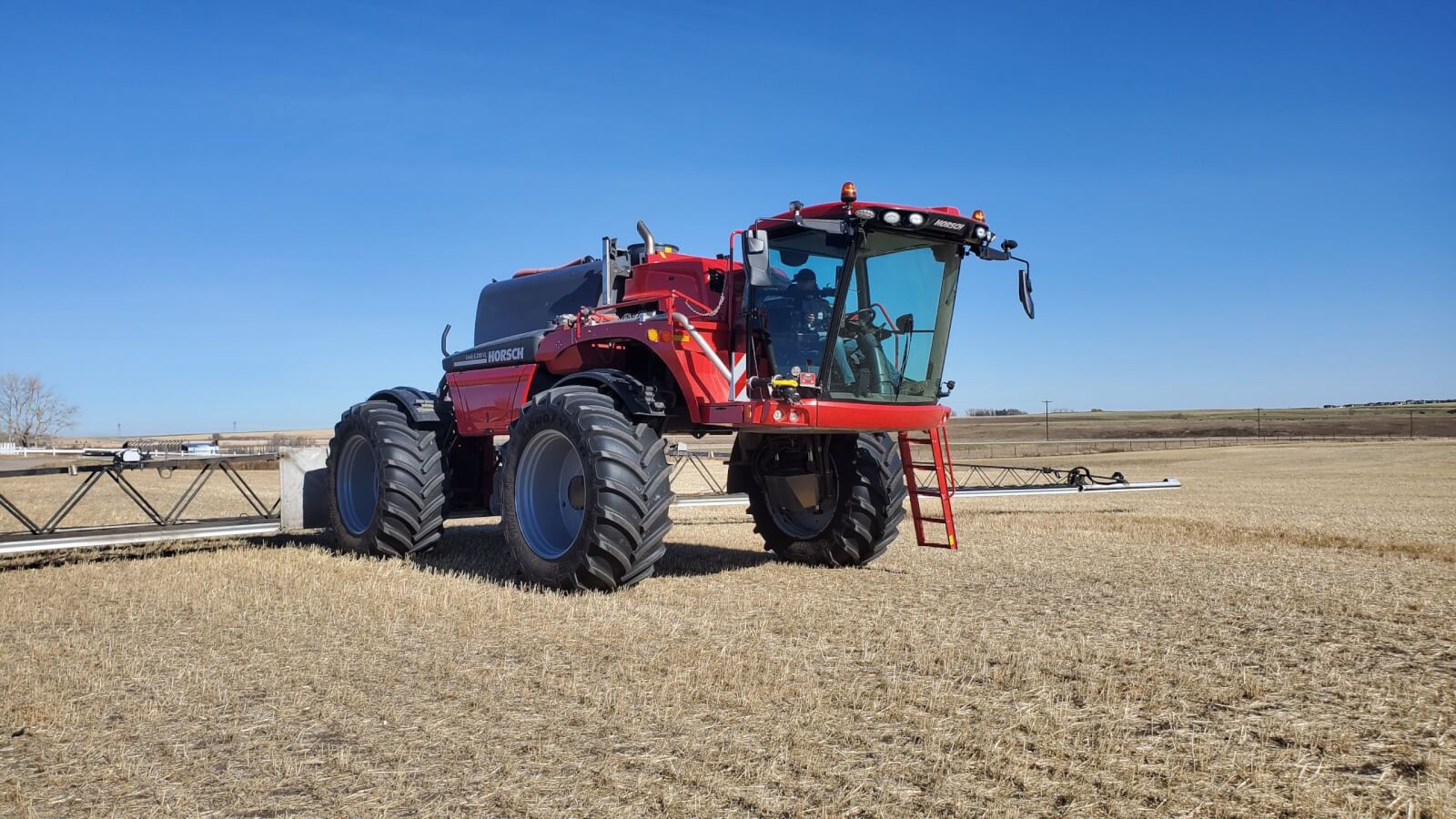
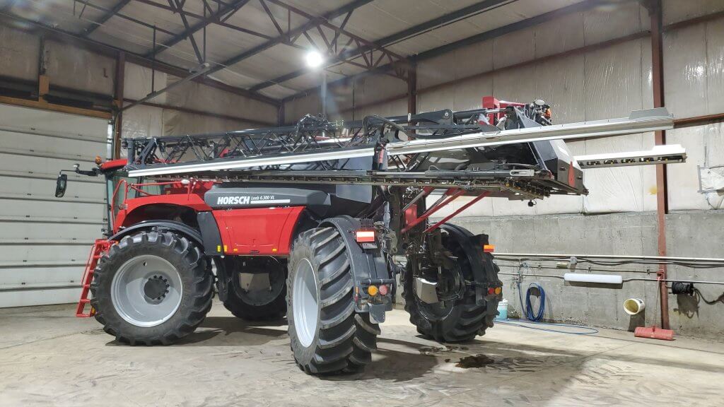
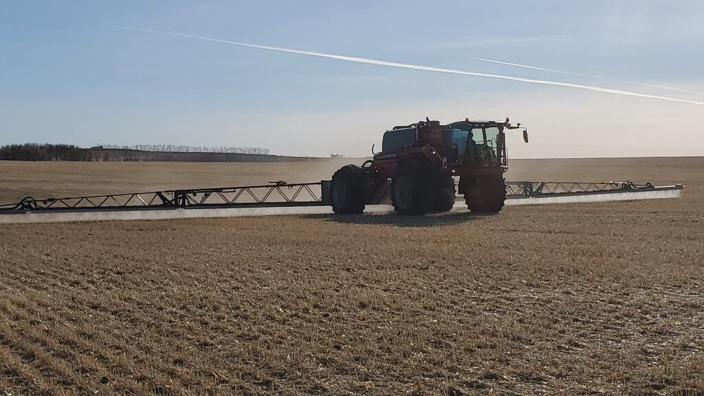
Their current flagship sprayer in North America is the Horsch Leeb 6.300 VL. I spent a day with Mike Wasylyniuk, Product Marketing Manager for Horsch, in Crossfield, Alberta to look it over.
The Numbers
The sprayer chassis holds a 1700 US gallon stainless steel tank and two 100 gallon clean water tanks for a total liquid capacity of 1900 gallons. A stainless steel Pentair Hypro centrifugal pump provides the flow to the boom, and a second pump is dedicated to the clean water tanks. The sprayer is powered by a familiar FPT 6.7 L producing 310 hp. The boom is 120’ wide in 5 articulated sections with 10’ nozzle spacing fitted with Raven Hawkeye Pulse Width Modulation (PWM). Top spraying speed is 20 mph, top transport is 30 mph. Horsch claims a dry weight of 32,000 lbs when fitted with Goodyear LSW 900 50R46.

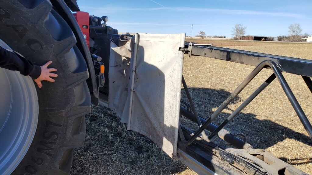
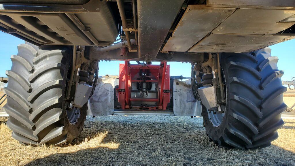
A central tubular frame creates room for four-wheel steer that has an interior turning radius of 3 m. Wheels are suspended via hydropneumatics linked to the frame with double wishbones. Track width adjusts from 120″ to 160″, independently, allowing different track widths front and rear without pinning an axle in place. Standing beside the front wheel, one has with easy access to fuel and oil filters, the radiator is on top of the machine facing up with an air-chuck outlet for cleaning.
Plumbing
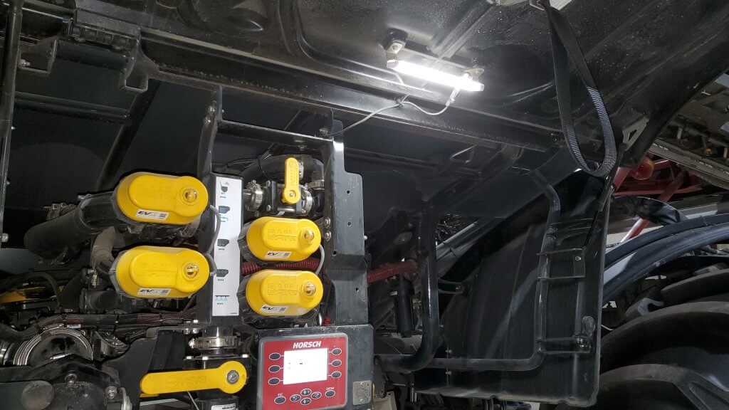
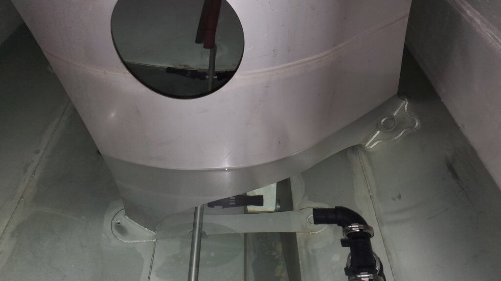
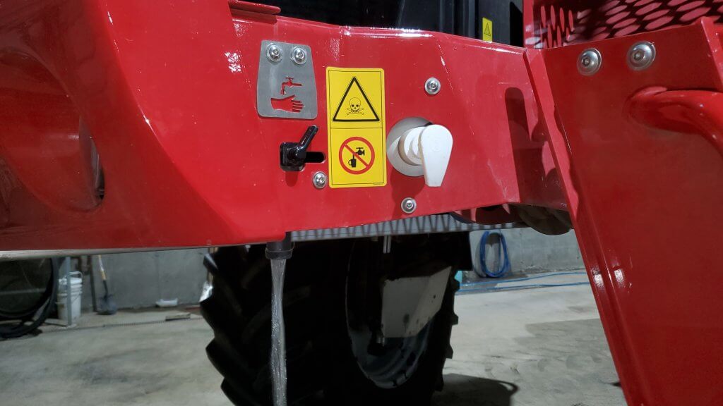
Any loyal reader of Sprayers101 knows that we believe the biggest room for improvement in spraying is in the plumbing. Horsch Leeb seems aware of this. First, it does away with sight tubes on the tank and relies on a more accurate digital float that reads down to an empty tank. Tank slope position is considered using a gyro mounted at the rear of the sprayer. The tank can be filled with the solution pump or from the tender truck using 3” side or front fill locations. It has auto shutoff when a target amount is reached. As is common, the majority of valves are motor operated to allow automation.
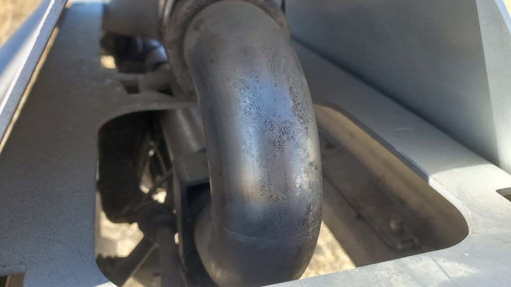
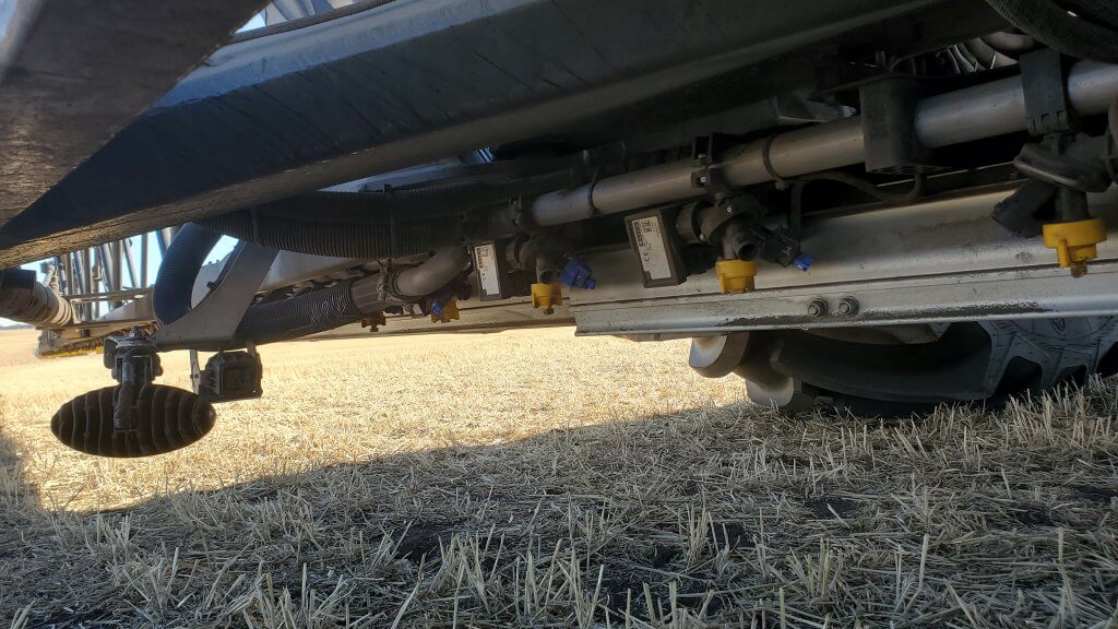
The recirculating boom plumbing is standard North American 1” OD stainless steel to suit any off the shelf nozzle body clamp. It pressurizes from both ends when spraying and returns to tank from the outside of the boom when nozzles shut off or when priming or flushing. The recirculation can run during transport, allowing boom priming en-route to the field, or continuous flushing with a cleaning solution in the main tank on the way home.
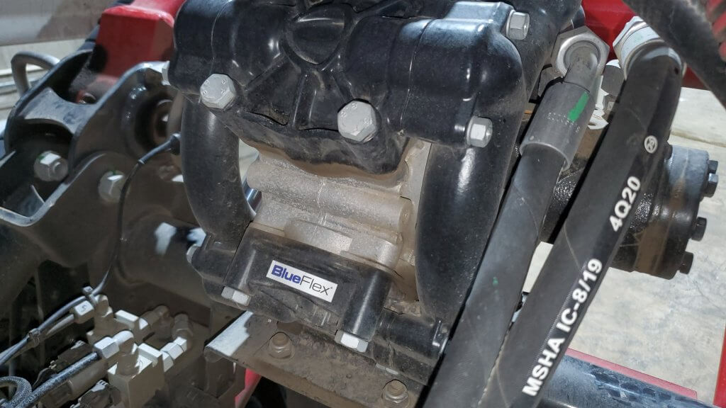
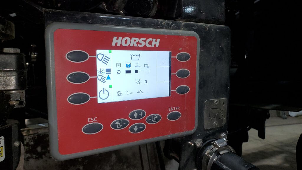
The second pump, an Italian Annovi Reverberi 185 BP diaphragm, powers the continuous cleaning function. It draws from the clean water tank and can push this water to the boom for overnight storage when the tank has solution left, or to the tank’s wash-down nozzles for a continuous clean at the end of a job. In continuous clean mode, the solution pump continues to supply the boom while the cleaning water washes the walls and dilutes the remainder. The tank and boom can be washed with a minimum of liquid, and the process is automated using cab or side monitor controls.
The system even has a winterizing button that controls all the necessary valves to distribute antifreeze from the clean water tanks throughout the plumbing system in minutes. Remaining antifreeze in the tank can be returned to the drum at the fill station with a convenient camlock drain.
Some may gloss over plumbing paragraphs in haste, but let’s not underestimate the magnitude of these features. We are talking about a plumbing system that can prime the boom without spraying, spray the field, then spray out any remainder while rinsing the tank, air purge the boom, then rinse the boom without leaving the cab or wasting material unnecessarily. Even the system strainers have flush capability that returns any residue to a removable fine mesh filter before the liquid dumps back to the tank. Such a design saves time and money and pays in acres per hour.
Boom
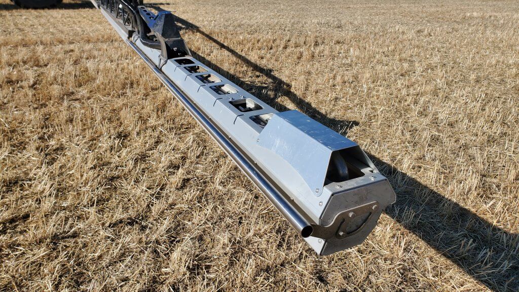
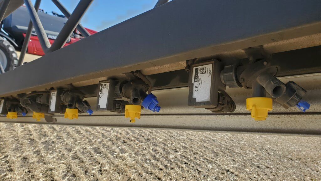
The 120’ boom is well built and has channels for wiring harnesses that are neatly zip-tied in place. An aluminum shield covers the nozzle bodies at the front to protect them from any ground contact. Access is relatively convenient through ports on the other side. The fitted triple nozzle bodies should be enough to suit most needs. The swing-away has a sturdy steel tube on the leading edge to absorb and deflect any sudden impact. There is no exposed plastic. The recirculating boom plumbing is stainless steel throughout except at hinges, where the rubber hose loop is protected from chafing by an additional sleeve.
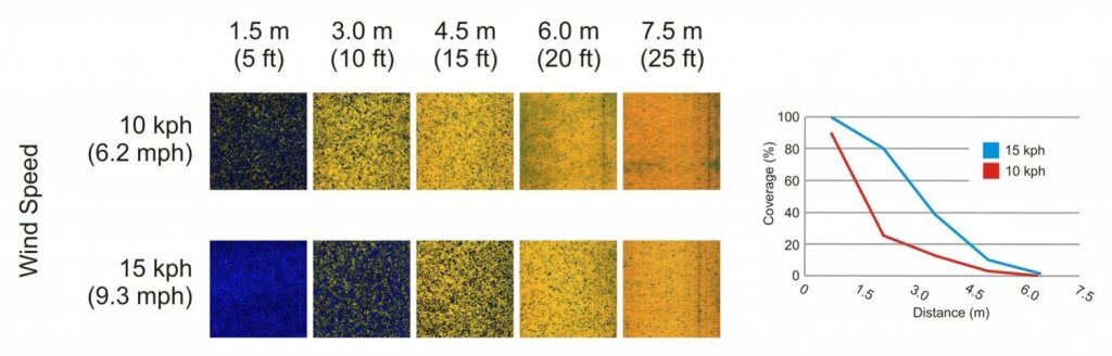
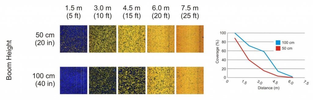
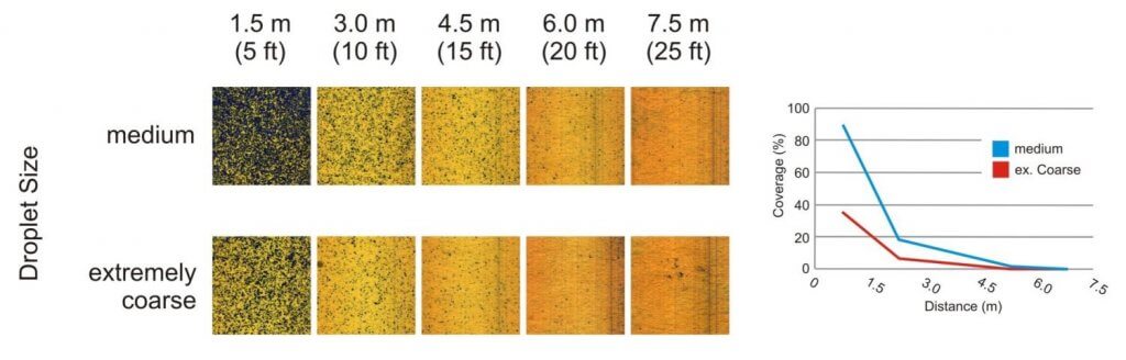
The Leeb philosophy is to design sprayers that control drift at the source without reliance on extremely coarse sprays that can hamper efficiency. They’ve chosen boom height as the key variable and built the boom to make this possible. First, they needed to design a system that can reliably hold the boom low and level.
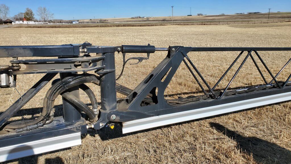
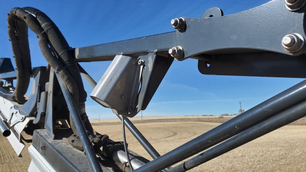
To that end, three pivot points are used to provide independence of the tractor unit and the boom. The first is at the centre rack from which the boom hangs but can pivot thanks to the same gyro that helps read the tank level. A sudden tractor movement due to ruts, for example, can then be compensated. The wings are the second pivot point (as it is for all sprayers), and a third point is halfway out the wings, where a hinge allows for up or down adjustments to better suit the land contour.

The height sensors have a modest look ahead slant, and the company claims that 8” boom height at 10 mph is possible. We certainly tried that in the field, and after multiple runs up and down a local field with modest knolls we did not strike ground, although the boom ends did rise significantly on occasion. The claim of such low booms will be a point of considerable testing and debate.
To take advantage of the low heights, narrower 10″ nozzle spacings are needed. The boom therefore has 144 nozzles instead of the usual 72, each half the flow rate. This is new territory for PWM, where the smaller tips are not as widely available. For example, a traditional 5 gpa tip at 20” and 12 mph is 03 in size, with 10” spacing this is now 015. Smaller sizes require more attention to filtering, and they have inherently greater drift potential. This would only be a problem at the lower application rates.
Because PWM allows for individual nozzle control, the operator can select 20” spacing, based on either of the 10” positions. This means one can spray with 20” spacing and then switch to a different nozzle simply by selecting the alternate.
The lower boom height can offer unique advantages. The first of these is drift control. Droplets emerge from the tip at about 70 km/h, and this initial speed prevents even the small ones from drifting. The higher the boom, the more they slow down before targetting, creating drift potential. Wind speeds also tend to be lower nearer to the ground.
Second, the beneficial effects of twin fans or angled single tips are greater with low booms. Readers will know that one of the fundamental prerequisites for successful angled sprays in Fusarium head blight (FHB), for example, are low booms. We may be in for some positive outcomes.
The User Experience
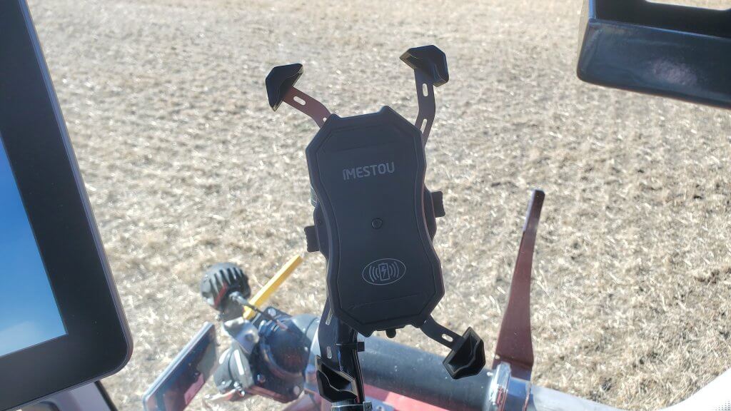
The Class cab has the usual creature comforts with a buddy seat, four cup holders, bluetooth radio and a phone mount. It can be fitted with any ISOBUS monitor, the one we had was equipped with the Raven Viper 4. The climb up the ladder is not as stair-like as the North American sprayers, but the treads are large and there are plenty of handholds so you can climb one-handed and bring your lunch or toddler along for the day.

There is one native Horsch monitor that controls the chassis, wheel spacing, engine specs, speed, etc. It’s controlled using a rotary button selector like the one in many cars, a wheel that highlights items by turning, then selects them with a push. The second, an ISOBUS monitor, handles the rate control and thus creates easy compatibility with a variety of aftermarket monitors.
The joystick is backlit and buttons can be customized. Like the Fendt stick, a push forward sets the speed and it can return to the neutral position without changing that speed. A pull back is required to slow down. It takes a bit of getting used to. Motion can also be foot operated with a speed pedal and foot brake. Cruise control has two preset speeds, and boom height can be raised to preset values when the master switch is shut off to facilitate a headland turn. The top two thumb buttons are Master on/off and autosteer resume.
There is no throttle control. The sprayer decides how much throttle is needed to maintain speed, saving noise and fuel when it can. Throttling up was noticeable as we climbed hills during our test drive, returning to lower rpm as we descended while maintaining our cruise control speed.
Some touches
- a hand wash station at the ladder to prevent contaminating the hand-holds or cab
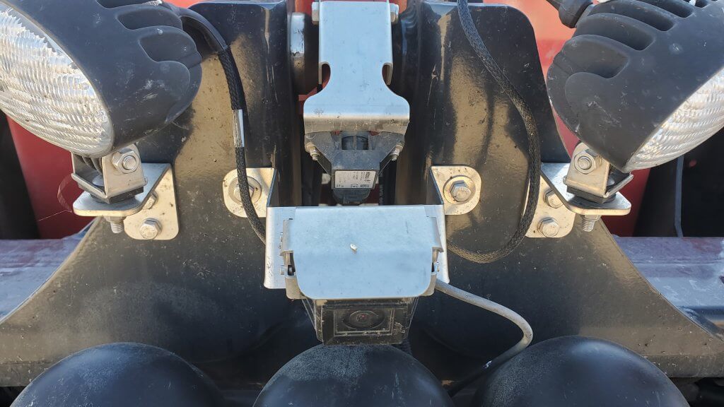
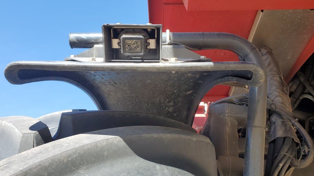
- a camera focused on the centre rack nozzles that are invisible from the cab
- cameras showing front wheel position
- mud guards behind rear wheels to protect boom
- Rain cover over electronics mounted on centre rack

- A clean underbelly with good clearance and tow hooks front and back
- Inductive (wireless) phone charging mount
Overall Impression
It’s clear that Horsch Leeb wants to succeed in North America. I’ve hardly ever seen a company so bent on delivering what the market wants (for familiarity and compatibility) while delivering what it knows they need (like plumbing and drift control). Spending the day with Mike I learned how quickly the engineers and fabricators implemented his suggestions at the factory. That is perhaps the most promising aspect of all, a company that listens to its customers and continually evolves its product as a result.