Download the 2023 publication from Crop Protection here.
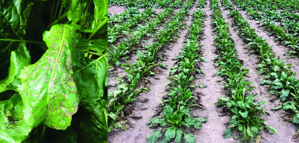
Cercospora leaf spot (CLS), caused by the fungal pathogen Cercospora beticola, is one of the most damaging foliar diseases affecting sugarbeet (Figure 1) (Khan et al. 2008). Growers rely on broad-spectrum contact fungicides because they are less likely to cause fungicide resistance (OMAFRA 2020). However, these fungicides are usually less effective than other fungicides (Trueman & Burlakoti 2014), and require frequent reapplications (Thind & Hollomon 2018) and good coverage to be effective (Prokop & Veverka 2006; Roehrig et al. 2018).
Figure 1. Cercospora leaf spot on sugarbeet.
We evaluated practices intended to improve the efficacy of Manzate® Pro-Stick™ (Mancozeb) by improving deposition and penetration into the sugarbeet canopy. Practices included different nozzle types (Shepard et al. 2006; Dorr et al. 2013), carrier volumes (Armstrong-Cho et al. 2008; Roehrig et al. 2018; Tedford et al. 2018) and the addition of InterLock®. InterLock is a spray adjuvant made with modified vegetable oil (MVO), vegetable oil and a polyoxyethylene sorbitan fatty acid ester emulsifier. It is intended to reduce the number of drift-prone, fine droplets without compromising the volume median diameter (WinField® 2019).
Research
In 2019 and 2020, InterLock and carrier volume were assessed to evaluate effects of:
InterLock on Manzate Pro-Stick efficacy at different carrier volumes.
InterLock on spray deposition and penetration within the sugarbeet canopy.
Objective 1: InterLock on Manzate Pro-Stick efficacy at different carrier volumes
Four replicated field trials were conducted at two sites, Dealtown (2019) and Ridgetown (2019 and 2020). Treatments were evaluated using four carrier volumes: 115, 235, 350, and 470 L ha-1 (12, 25, 37, and 50 gpa) and applied on a 14-day schedule.
Results
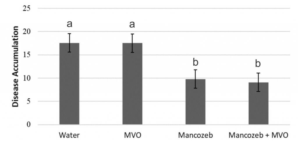
Adding InterLock to Manzate Pro-Stick did not reduce disease accumulation over the season (Figure 2a) or improve beet and sugar yield or sugar quality compared to applications of Manzate Pro-Stick alone (data not shown).
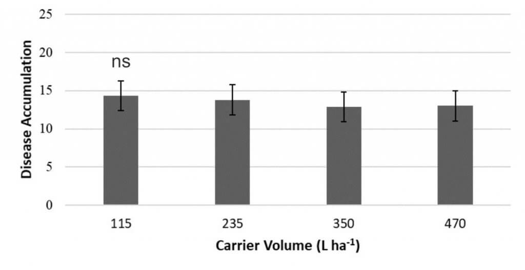
Carrier volume did not affect disease accumulation (Figure 2b).
Figure 2a. Disease accumulation (standardized area under the disease progress stairs; sAUDPS) (±SE) for fungicide treatments applied to sugarbeets in Ridgetown and Dealtown ON 2019, and in Ridgetown 2020. Bars followed by the same letter are not significantly different at p ≤ 0.05, Tukey’s HSD, ns= not significant.Figure 2b. Disease accumulation (standardized area under the disease progress stairs; sAUDPS) (±SE) for carrier volume applied to sugarbeets in Ridgetown and Dealtown ON 2019, and in Ridgetown 2020. Bars followed by the same letter are not significantly different at p ≤ 0.05, Tukey’s HSD, ns= not significant.
Objective 2: InterLock on spray deposition and penetration within the sugarbeet canopy
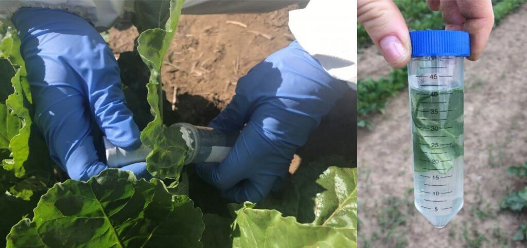
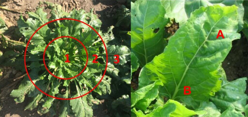
Deposition was evaluated using Rhodamine WT dye recovery. The amount of dye recovered for a treatment (µL AI/ g leaf tissue) was used to make assumptions about treatment deposition in the sugarbeet canopy. To assess spray deposition, samples were taken from six canopy locations (Figure 3 and 4).
Figure 3. Leaf sample collection from sugarbeet canopy.Figure 4. Leaf samples were taken from a) three canopy locations 1= inner, 2= mid, 3= outer from b) two leaf locations each A= tip, B= base.
Three sets of replicated experiments were conducted in Ridgetown (2019 and 2020) to evaluate the effect of InterLock on canopy deposition when 1) mixed with Manzate Pro-Stick, 2) using three different nozzle types, and 3) using three carrier volumes.
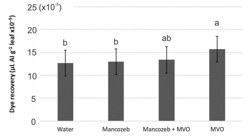
In the first study, four programs (Manzate Pro-Stick + InterLock, Manzate Pro-Stick alone, InterLock alone, and water) were evaluated for dye recovery.
Results
Deposition was improved for the InterLock only treatment compared with water, but when InterLock was applied with Manzate Pro-Stick the deposition was the same as Manzate Pro-Stick applied alone (Figure 5). It is possible that the fungicide formulation or active ingredient had an antagonistic effect with InterLock, though we cannot determine that from this study.
Figure 5. Effect of program on mean Rhodamine WT active ingredient (µL per gram of dry leaf) (±SE) recovered from six locations in a sugarbeet canopy at the 13 (Trial 1) and 16 (Trial 2) leaf stage in Ridgetown, ON 2019. Bars followed by the same letter are not significantly different at p ≤ 0.05, Tukey’s HSD.
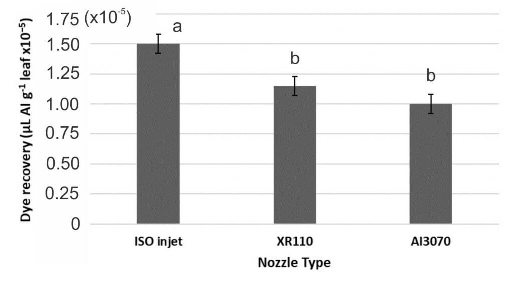
In the second study Manzate Pro-Stick + InterLock and Manzate Pro-Stick were applied using three different nozzle types at ~40 psi:
The Hardi ISO Injet is an air inclusion 110° flat fan that produces a Very Coarse spray quality.
The TeeJet XR110 is a conventional 110° flat fan that produces a Medium spray quality.
The TeeJet AI3070 is an air inclusion, dual flat fan (30° and 70° spray angles) that produces a Coarse spray quality.
Results
Adding InterLock did not affect deposition and did not alter the performance of any nozzle type (data not shown).
Deposition among nozzles did differ, with the ISO injet nozzle providing improved deposition compared to the XR110 and AI3070 nozzles (Figure 6).
Figure 6. Effect of nozzle type on mean Rhodamine WT active ingredient (µL per gram of dry leaf) (±SE) recovered from six locations in a sugarbeet canopy at the 15 (Trial 3), 18 (Trial 4), and 19-22 (Trial 5) leaf stage in Ridgetown, ON 2019 and 2020. Bars followed by the same letter are not significantly different at p ≤ 0.05, Tukey’s HSD.
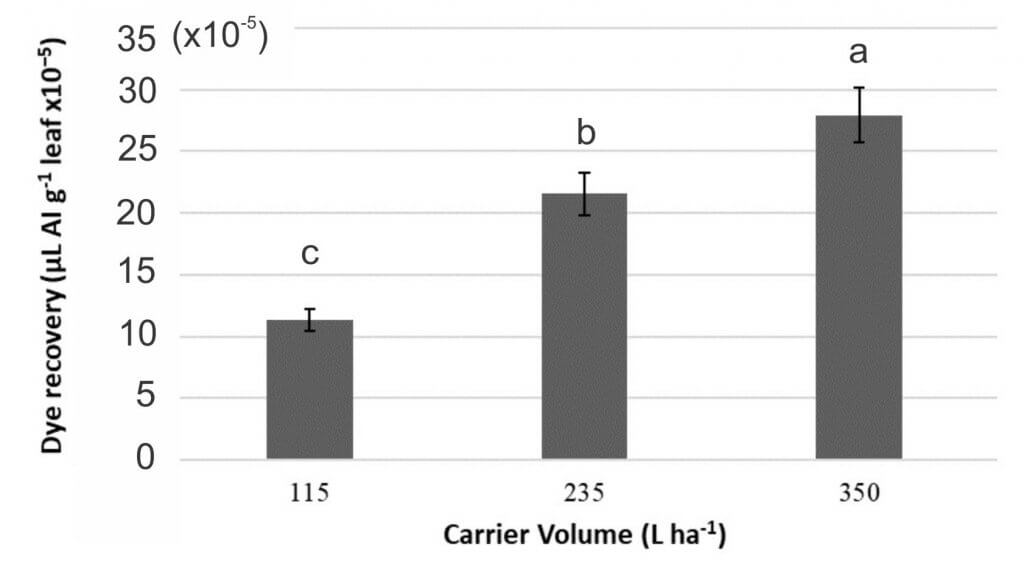
In the third study, Manzate Pro-Stick + InterLock and Manzate Pro-Stick were applied using three carrier volumes: 115, 235, and 350 L ha-1.
Results
The addition of InterLock had no effect on deposition, regardless of carrier volume (data not shown).
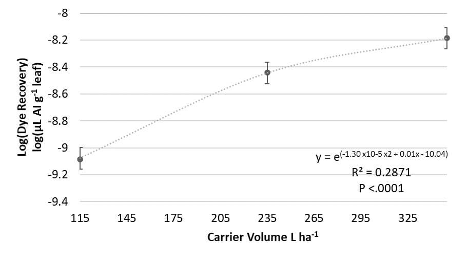
Deposition increased with increasing carrier volume (Figure 7a). A regression analysis determined a curvilinear relationship between carrier volume and deposition, predicting that deposition would increase with increased carrier volume until a maximum carrier volume was reached (Figure 7b). Many studies indicate that at exceptionally high carrier volumes coverage can be reduced primarily due to run-off.
Even though increased carrier volume improved fungicide deposition, increased volume did not improve fungicide efficacy for CLS management (Objective 1 efficacy trials).
Figure 7a. Effect of carrier volume on mean Rhodamine WT active ingredient (µL per gram of dry leaf) (±SE) recovered from six locations in a sugarbeet canopy at the 20 and 23 leaf stage in Ridgetown, ON 2020 (Trial 6 & 7). Bars followed by the same letter are not significantly different at p ≤ 0.05, Tukey’s HSD.Figure 7b. Regression of carrier volume (115, 235, 350 L ha-1) and mean Rhodamine WT active ingredient (±SE) recovered from six locations in a sugarbeet canopy at the 20 and 23 leaf stage in Ridgetown, ON 2020 (Trial 6 & 7). Data analysis was performed on the log normal scale, means and SE presented have not been back-transformed.”
Canopy location was an important factor in all experiments
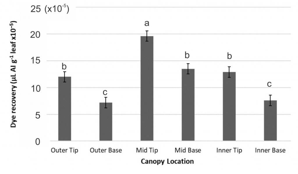
The least deposition was always found in the outer and inner canopy from the base of the leaf, and in the outer canopy from the tip of the leaf (Figure 4), suggesting that these locations are the most challenging to achieve spray deposition. An example from the nozzle type experiment is shown in Figure 8. One of the proposed benefits of InterLock is for improved spray penetration, but in the current study, InterLock did not improve penetration of Manzate Pro-Stick into any of the harder to reach canopy locations.
Figure 8. Effect of canopy location on mean Rhodamine WT active ingredient (µL per gram of dry leaf) (±SE) recovered from six locations in a sugarbeet canopy treated with InterLock and different nozzle types at the 15-22 leaf stage in Ridgetown, ON, 2019 and 2020 (Trials 3, 4 & 5). Bars followed by the same letter are not significantly different at p ≤ 0.05, Tukey’s HSD.
Conclusion
Adding InterLock to Manzate Pro-Stick did not improve deposition in any field experiment regardless of the nozzle type or carrier volume used. Further, using InterLock with Manzate Pro-Stick did not improve fungicide efficacy for CLS management. However, we cannot determine from this study if InterLock would improve deposition, penetration, or fungicide efficacy using other fungicide products.
Despite findings of improved disease management with the use of larger carrier volume, fungicides are sometimes still applied with smaller carrier volumes of 100 L ha-1 or less (Armstrong-Cho et al. 2008; Roehrig et al. 2018) to save time and reduce the cost of application. In this experiment, increased carrier volume improved deposition but did not improve fungicide efficacy of Manzate Pro-Stick for CLS management. There is the potential that using increased carrier volume may be more beneficial in years with a greater disease severity, and may thus be worthwhile to growers, as has been observed in previous research on Cercospora leaf spot in Ontario (Tedford et al. 2018).
This research was sponsored from the Canadian Agricultural Partnership, Ontario Agri-Food Innovation Alliance, Ontario Sugarbeet Growers’s Association, and the Michigan Sugar Company.
References
Armstrong-Cho C, Wolf T, Chongo G, Gan Y, Hogg T, Lafond G, Johnson E, and Banniza S. 2008. The effect of carrier volume on Ascochyta blight (Ascochyta rabiei) control in chickpea. Crop Prot. 27: 1020-1030.
Dorr GJ, Hewitt AJ, Adkins SW, Hanan J, Zhang H, and Noller B. 2013. A comparison of initial spray characteristics produced by agricultural nozzles. Crop Prot. 53: 109-117.
Khan J, del Rio LE, Nelson R, Rivera-Varas V, Secor GA, and Khan MFR. 2008. Survival, dispersal, and primary infection site for Cercospora beticola in sugar beet. Plant Dis. 92: 741-745.
Ontario Ministry of Agriculture, Food, and Rural Affairs (OMAFRA). 2020. Vegetable Crop Protection Guide, Pub 838. Sugarbeets. Queen’s Printer for Ontario, Toronto.
Prokop M, and Veverka K. 2006. Influence of droplet spectra on the efficiency of contact fungicides and mixtures of contact and systemic fungicides. Plant Protect. Sci. 42: 26-33.
Roehrig R, Boller W, Forcelini CA, and Chechi A. 2018. Use of surfactant with different volumes of fungicide application in soybean culture. Eng. Agr. Jaboticabal 38: 577-589.
Shepard D, Agnew M, Fidanza M, Kaminski J, and Dant L. 2006. Selecting nozzles for fungicide spray applications. Golf Course Manag. 74: 83-88.
Tedford SL, Burlakoti RR, Schaafsma AW, and Trueman CL. 2018. Optimizing management of Cercospora leaf spot (Cercospora beticola) of sugarbeet in the wake of fungicide resistance. Can. J. Plant Pathol. 41: 35-46.
Thind TS, and Hollomon DW. 2018. Thiocarbamate fungicides: Reliable tools in resistance management and future outlook. Pest Manag. Sci. 74: 1547-1551.
Trueman CL, and Burlakoti RR. 2014. Evaluation of products for management of Cercospora leaf spot in sugarbeet, 2014. Plant Disease Management Reports. 9: FC009.
WinField United. 2019. InterLock. [Internet]. [cited 2019 Feb 25].
The self-propelled sprayer revolution is complete in western Canada. Almost all sales of new equipment are self-propelled. In fact, the once thriving sector of Canadian-made pull-type sprayers, and the innovations they brought to spraying, has disappeared.
In its place we have self-propelled sprayers that offer plenty of power, large tanks, high mobility and comfort, and of course, the clearance required for late-season sprays. These features come at a cost: high capital expense, weight, fuel consumption and drift potential if the speed or boom height are not controlled.
The self-propelled machines are nice; however, customers are becoming concerned about overall value. Sure, the sprayer is the most-used piece of equipment on the farm, with the average field being treated four to five times per year. Does that justify the $500 to $700 k purchase price?
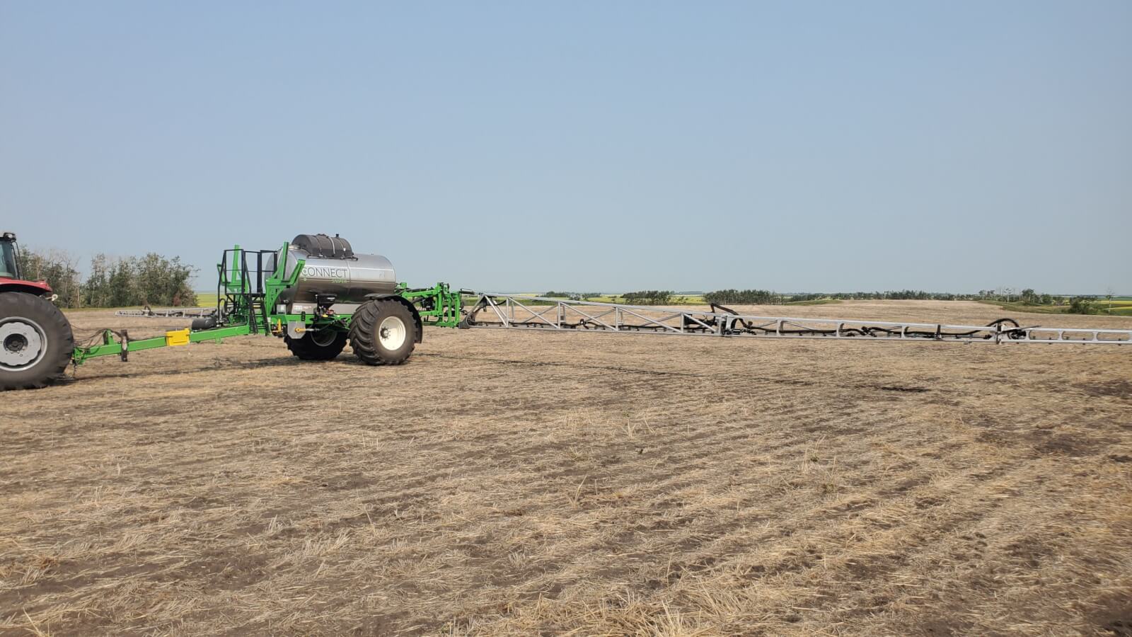
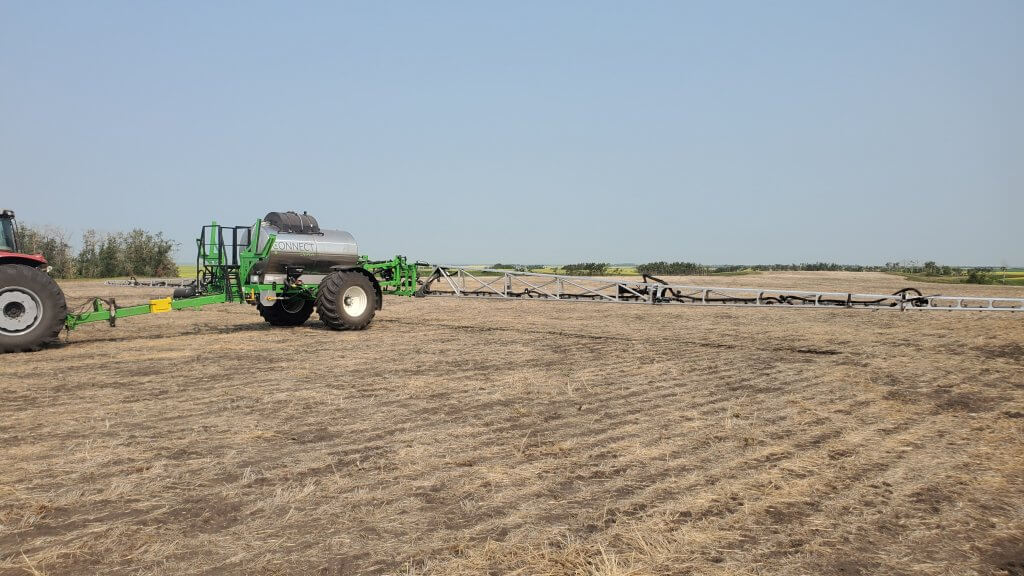
To answer this question, we need to evaluate the alternatives. Even though we’ve lost most North American pull-type sprayer makers, a few, such as Top Air, are left. A new pull type, the Connect Sniper, is being offered by Pattison Liquid. In addition, there are now several European manufacturers looking at our market. These bring large capacity, sophisticated booms plumbing and a narrow transport width. Let’s look at the issues:
The Connect Sniper, manufactured by Pattison Liquid, offers recirculating booms, Raven Hawkeye pulse-width modulation, continuous rinsing, and 120′ Millenium booms. The WEEDit spot spray system is also available.
Capacity
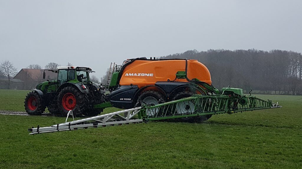
Not a problem. Top Air features tanks up to 2400 gallons and 132’ booms. Amazone builds a 3000 gallon tank twin axle sprayer (UX11200) with 132’ booms. The 230 gpm on-board diaphragm pump can fill the sprayer in 15 minutes. The Hardi Commander offers tanks up to 2600 gallons with 132’ booms. The Horsch Leeb TD12 is at 3170 gallons with 138’ booms. Equipped with air brakes, these sprayers can be trailed at up to 50 km/h.
The Amazone UX 11200 has an 11,200 L (2960 US gal) tank and tandem, steering axles combined with up to 130′ booms.
Clearance
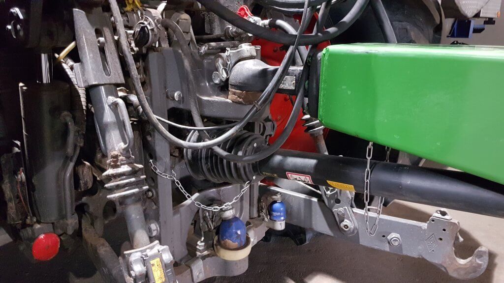
The pull-types themselves have adequate clearance for most crops. The limiting factor will be the tractor and the hitch point. The availability of a high hitch point, and an 80 mm ball, on European tractors, is a boon for this. Although it may be necessary to shield the low standard drawbar and belly, pull-type owners report no long-term effects from the lower clearance.
The Horsch Leeb TD12 offers a 12,000 L (3170 US gal) tank and up to 1.25 m ground clearance (Photo: Horsch.com).European tractors offer 80 mm ball hitches for larger implements with high mounting heights to gain extra sprayer clearance.
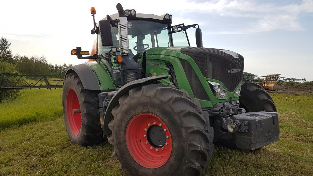
Tractor
The pull-type sprayer makes most sense if it allows the re-purposing of an existing tractor. The common yard tractor isn’t enough, as the high capacity sprayers may require >200 hp with front wheel assist, especially in softer ground or hilly terrain. Another requirement is that the track width match the sprayer, and the European standard of a 2.25 m track width (centre to centre) can be hard to match in North America. New rims on the sprayer can push the width out, but the resulting increased axle stress may be problematic; these issues should be considered in advance. Fortunately, powerful front wheel assist tractors are finding a place on farms, even as seeding tractors. The changing over from one implement to another during a busy time can be a hassle, with a dedicated rate controller requiring additional cab real estate. But with the lower capital cost of a pull-type, a new tractor that also has other utility on the farm may be justified.
Large pull types require large tractors that may not already exist on the farm. The ability to match wheel tracks and the convenience of monitor hookups are important considerations.
Productivity
We’ve long maintained that productivity gain through increased travel speed creates more problems than it solves. It is virtually unavoidable to use somewhat higher booms with faster speeds, and it’s been proven that spray drift potential increases with travel speed. Instead, the sprayer features that save time are faster fill and clean times (reduced downtime), larger tanks (fewer stops to fill) and wider booms. Wider booms are easier to keep steady with slower moving equipment.
So how do typical self-propelled sprayers stack up against pull-types?
We compared two sprayers, a large pull-type with 3000 US gallon tank and a typical self-propelled with a 1200 gallon tank. Travel speeds were 10 and 15 mph, respectively, and fill times were 15 and 10 minutes. The slower pull-type turned in one headland, whereas the self-propelled used two to allow room for acceleration after the turn.
On half-mile runs, our “Productivity Calculator” at agrimetrixapps.com showed 129 acres per hour for the self-propelled and a respectable 119 acres/h for the pull type. The value of fast but infrequent fills and the more efficient turns made the difference for the pull-type. Use the app to compare other tank sizes, travel- and fill-speeds, or boom widths.
Productivity of a 3000 gallon tank pull-type (left) vs a 1200 gallon self-propelled (right), given specific speed, boom width, and fill times.
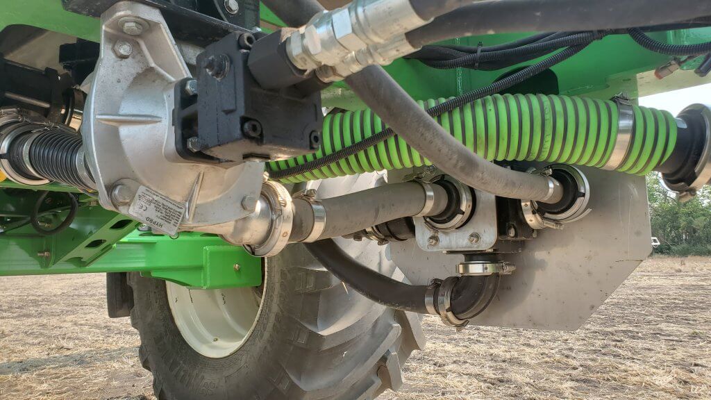
The specific design features of a sprayer may create additional productivity. For example, the ease of tank rinsing and cleanout can save time. European sprayers typically have lower remaining volume values, which increases the speed of tank rinsing and can eliminate the need for dumping tank remainders on the ground. Ease of filter inspection may seem trivial, but it permits more frequent confirmation that the system is clean and thus avoids potential future problems. An on-board pressure washer on the Amazone makes boom hygiene easier. It’s important to account for all these seemingly small gains because they add up.
Service
The success of any agricultural equipment relies on the equipment durability, fast availability of parts and service. Any new market entry will need to establish a dealer network, parts distribution system and superior service. This is no easy feat in a time of dealer consolidation. But without a drive train, there’s less to go wrong in a pull-type, and many plumbing parts are generic or can be obtained in metric equivalents.
With fewer mechanical components, pull-type sprayers require less service and are less prone to breakdowns.
Cost and Value
Prices vary, but a pull-type sprayer will usually cost less than half of a similar-sized self-propelled sprayer depending on the options selected.
With European-influenced equipment, the plumbing system will be more sophisticated, often offering recirculating booms, steering axles that follow in the tracks of the sprayer, narrow transport widths for greater road safety, an improved boom suspensions and levelling performance. It is safe to say that in terms of features, these sophisticated machines offer good value and many good design ideas. Operating costs are almost certainly lower, with better fuel economy and less drivetrain trouble.
The pull-type sprayer continues to have an important place to fill on our farms. With trade and weather anomalies lowering farm income, farmers are wary of being over-capitalized. It is conceivable that lower-cost and feature-rich alternatives to self-propelled units will have a fit. They certainly make sense on smaller farms that may not be able to utilize the full performance of a self-propelled, or on a larger farm that needs extra capacity but doesn’t want to bear the capital cost of a second expensive sprayer. The inherently slower working speeds allow for lower booms, less drift, overall improved deposit accuracy and uniformity. They’re worth a closer look.
How much horsepower (HP) do you need (really) when pairing a tractor and a towed sprayer or any other PTO powered implement? This important question should be asked BEFORE purchasing any towed implement. Surprisingly, there’s not much guidance out there, so you might hear answers like:
Whatever my tractor has must be enough… whatever that happens to be.
What?
The right amount of HP is what I can afford. Erma, grab that milk can full of egg money…
MOAR! (Yes, we know how “more” is spelled, but memes are funny).
Skeletor knows horsepower
Rating Tractor Horsepower
If you thought there was only one way to rate the horsepower of a tractor, well, you’d be wrong. At its simplest, horsepower is:
(torque × engine revolutions) ÷ a constant
We’ll expand on this later. The rub comes in how you define each of these factors and where you measure the power. Let’s start with something simple like engine speed, which is expressed in Revolutions Per Minute or RPM’s.
Engine Speed
So, if horsepower is the result of torque times engine speed, what speed do the manufacturers plug into the formula? One of two values are used:
1. Power Take-Off (PTO) Engine Speed
This is the engine RPM’s that produce the rated operating speed on the PTO. When the PTO is engaged, the engine is directly and mechanically connected to the PTO shaft. Therefore, maintaining the engine at the rated PTO speed, typically between 1,500 and 2,300 RPM depending on if it’s gas, diesel, turbocharged or not, will keep the PTO spinning at a uniform 540 or 1,000 RPM (the two typical PTO speeds) regardless of the driving speed.
2. Maximum Engine Speed.
This is the engine’s maximum intermittent operating speed… just shy of destroying said engine. An engine rated using the maximum speed gives you a false sense of security, because to get that horsepower you’ll be burning a ton of diesel, over-speeding your PTO implement, and wearing your tractor out very, very quickly.You wouldn’t drive your car around town in low gear because you’d redline the engine. Why would you do it to your tractor?
In the speedometer/tachometer (above the steering wheel) on this beautiful old tractor, the first black bar is the PTO rated RPM. The second is PTO Max. Operating with the PTO engaged above PTO Max can be damaging to the implement and to the tractor, and dangerous for the operator.
Horsepower Basics
OK, now we are ready to dig in a little deeper into defining tractor horsepower. What does it mean if, for example, your tractor is rated at 65 HP? We’ll skip the history lesson on watching the output of horses over an average day and move to the modern definition. Horsepower from a rotating shaft (such as the output of an engine) is:
Horsepower = [Torque in foot-pounds × Engine speed in Revolutions Per Minute (RPM)] ÷ 5,252
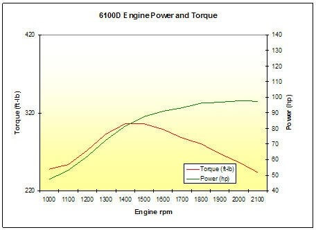
Here is a typical tractor torque curve. Notice how after peak torque, RPM’s climb quickly but net HP doesn’t. Unless specified, we can assume this is Engine Horsepower, not PTO Horsepower. If the above Torque/HP curves were your tractor, the PTO speed would likely be 1,500-1,600 RPM. According to the graph that would equate to about 82 HP. Running the engine up by 40% (2,100 RPM which is the max speed in this case, gets you about 98 horsepower. That’s only a 20% improvement. Remember, this is engine horsepower, not PTO horsepower, so this may not all be available for you to use. Image from JD.
Total Versus PTO Horsepower
Perhaps our tractor’s 65 HP rating describes Engine Peak Horsepower. This is what the engine would produce on a test stand, and it likely uses the maximum engine speed. This rating is a bit disingenuous. Not only because you will probably operate it at rated PTO engine speed, but also because some power is lost to internal processes, like the power steering pump, automatic transmission pump, alternator, auxiliary hydraulics, et cetera. So peak engine horsepower isn’t usually a very useful number unless you are in marketing and like big numbers.
A more accurate and useful rating is the Power Take-Off (PTO) Horsepower. This is the amount of horsepower available to do work at the PTO shaft. This may be at the rated PTO engine speed or the PTO Maximum speed. Estimating power using either speed offers a much more realistic rating of what you have to work with. As previously noted, PTO Rated Speed is usually near the speed where the engine creates the highest torque per revolution. This is often called the Power Band. Operation in this engine speed range will use the least diesel and result in the greatest amount of life in the machine.
Another important thing about PTO Horsepower is that this is the total amount of power available to do work. This could all go to PTO when the tractor is standing still, but both locomotion and the horsepower required to run the implement need to be subtracted from this number. So if your tractor is indeed 65 PTO horsepower, that’s the actual amount of horsepower you likely have to work with in real life.
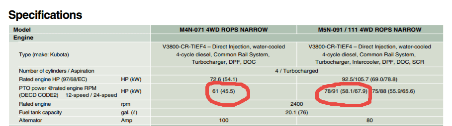
In this excerpt from a Kubota Spec sheet, you see that the Rated Engine horsepower is quite a bit higher than the PTO horsepower. A 72 HP “rated” tractor really has 61 horsepower for you to work with. The 106 horsepower version on the right really has 91 PTO horsepower.
The Horsepower that Matters
To sum things up, PTO Horsepower is the number you really need to care about. All this up to now just to describe the nuances of how horsepower is expressed. No wonder HP is a topic that’s avoided. If you can find or download the manual, now you at least have the tools to get to how much horsepower you have to work with.
Maximum Load
In order to answer the question of how much HP you need, you must consider your operation. You need to size your tractor for the biggest load it will ever be used for, even if you only do that thing once a year. Typically this would be a sprayer, rotavator or a brush flail. The rest of the year you won’t burn much extra diesel if you aren’t using the power in a bigger tractor, but you can’t draw on horsepower that isn’t there in a smaller one.
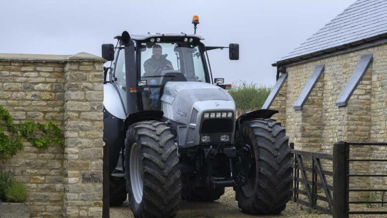
Though it’s not common, you can have too big a tractor. You need only watch “Clarkson’s Farm” for ample evidence (and a chuckle).
The enormous and infamous Lamborghini tractor that starred in “Clarkson’s Farm” on Amazon Prime is a good example of taking horsepower a little too far.
The Basics of Estimating Load
Now that you have the extremes in mind, let’s get to scratchin’. There are three things you must know to determine the maximum load:
Locomotion – The power needed to move the tractor and implement
Implement Power – The power needed to operate the implement
Safety Factor – This is a buffer that gives us a little extra just in case.
For the following guesstimates let’s assume you are doing orchard and vineyard work with a compact/narrow tractor. There really aren’t any hard and fast equations for this, but these will get you in the ballpark. If you are a nut grower with full sized tractors or a vegetable/field crop grower, you may need to scale up.
Locomotion
People discount it, but the power required just to move the tractor and the implement around is substantial. If the implement is a fixed tower sprayer with a 500 gallon tank, this might require 15-20 HP on flat, dry land. If your topography includes hills, or your terrain includes mud or tall grass, you may need to double that requirement. 45 HP just to move around before you even engage the PTO. Speed matters, too; If you are driving 5 mph, you’ll need twice the HP versus driving 2.5 mph.
The manufacturer of the implement should be able to tell you how much horsepower the implement requires. Small, three-point hitch airblast sprayers may only require 10-15 PTO HP. Larger tower sprayers may require 40-50 PTO HP. Brush flails may take 25-45 HP.
This is where things can get sticky and you need to make sure you’re both talking the same language. Some manufacturers will tell you how much power the implement takes, others will skip all the steps in this article and go right to recommending the size tractor they think you’ll need. If you’re unsure, ask. Be sure to factor in the locomotion requirements discussed earlier, the dealer may not understand your conditions in their general recommendation but usually can provide some clarity with a little more information from you.
Safety Factor
It’s always a bad idea to run at 100% of your power capability. Most of you reading this article are likely working with mid-life or older tractors with a few thousand hours on them. Ol’ Bessie loses some of the pep in her step over time. After engine break-in, the tractor will slowly lose power capability over its life. The harder you work it, the faster this occurs. Enthalpy happens (now that’s a great tee-shirt idea). Plan for it. Once you have an idea of your worst-case locomotion and implement power needs, add them up and give yourself another 15% (That is, multiply by 1.15).
Summing It Up
Now we can finally answer the question. In order to determine how much tractor horsepower you need, follow these steps:
Understand the real PTO horsepower of the tractor you are considering. This is the only thing that matters. You should be able to find online documentation for this if it doesn’t come with the tractor or you’ve filed it somewhere that you’ll never forget…
Establish the maximum load you are likely to encounter. Calculate this by multiplying the sum of Locomotion and Implement Power requirements by a 1.15 Safety Factor.
If you are still unsure, discuss these factors with your trusted local tractor dealer, ensuring you are both speaking the same language. It is better to err on too much tractor than not enough, but do so within reason.
Looking at our original orchard application with a 500 gallon tank and a larger tower type sprayer, travelling around 3 mph:
35 HP for locomotion, 40 HP to run the sprayer and 15% safety puts us at 35 + 40 + [0.15 × (35+40)] = 86.25 PTO HP
Wishing you all MOAR POWER and perfect spraying weather.
This is the final part of our three-part article discussing methods for digitizing and processing water sensitive paper. You can read part one here and part two here.
Morphological operations
We can now move on to the larger shapes, or “morphology” of the objects in our binary image. Our goal is to quantify deposits by interpreting these shapes. Once again, these operations are powerful processing tools, but we must acknowledge three overriding limitations:
1. Inconsistent stains
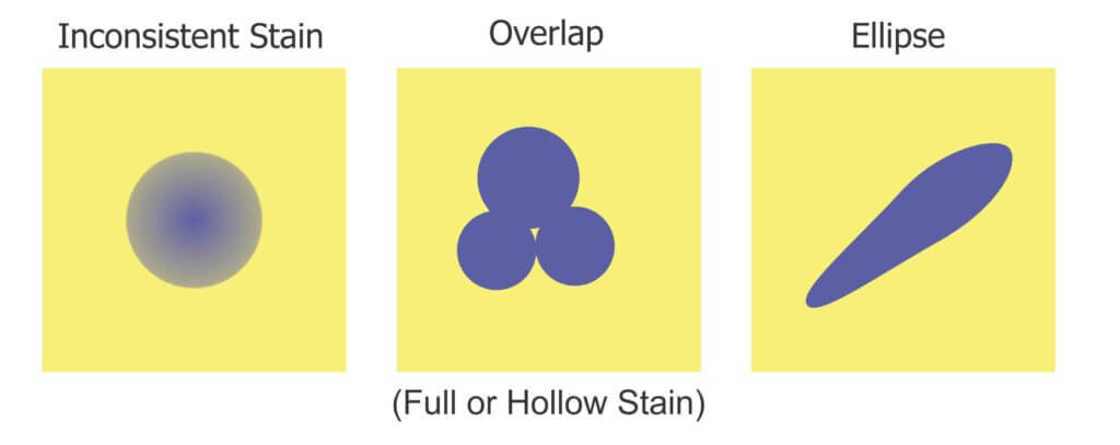
Sometimes deposits do not create a consistent blue colour – they can get lighter or take on a greenish-yellow hue towards the perimeter of the stain. During thresholding, the outer edge can be accidently eroded, leaving behind an object with a jagged edge. This may lead us to underestimate the percent area actually covered. In the case of tiny stains, it might eliminate them entirely and lead us to underestimate deposit density.
2. Overlaps
It can be difficult to determine if an object represents a stain from a single droplet or is the result of multiple, overlapping deposits. This becomes significant when the surface of the WSP exceeds ~20% total coverage. The resulting objects may or may not have hollow centres where droplets do not overlap entirely. Misidentifying overlaps leads us to falsely conclude that an object is the result of a single, coarser droplet rather than multiple finer droplets.
3. Ellipses
Non-circular stains are formed when droplets scuff along the surface. Two droplets with the same volume encountering a paper at different angles can create stains with significantly different areas. We may wrongly conclude that the droplets that created them were coarser than they truly were. One approach is to use Feret’s Diameter (aka Caliper Diameter) by measuring the widest spans on the X and Y axes and taking the average. Another approach is to interpret the ellipse as a series of circular stains. Or we can decide to only acknowledge these objects when calculating percent area covered, but omit them when calculating deposit density or predicting original droplet size. Each strategy is a compromise, so it is important to be consistent and transparent when reporting results.
Three common problems when analysing water sensitive paper.
We’ll explore two morphological operations that can help us separate fact from fiction: Granulometry and Dilation-and-Erosion. We’re introducing these operations as part of the processing and detection step, but they may also overlap with the measurement step in our three-step process.
Granulometry
We can estimate the range of object sizes and get a sense of how they are distributed on the paper by filtering or “sieving” the image. Imagine pouring a mixture of sand and rocks through a series of ever-finer sieves. Doing so allows you to separate particles based on size exclusion. A granulometry function compares each object to a series of standardized objects with decreasing diameters. This isolates objects of a similar size and bins them in that size range. This is a powerful operation, but accuracy is lost when stains overlap to form larger objects. In this case, we move on to Dilation and Erosion.
Dilation and Erosion
Think of dilation as adding pixels to the boundary of an object. This makes tiny objects bigger, fills in any interior holes and can cause objects to merge. The number of pixel-wide dilations required to make objects contact one another can be used as a measure of deposit density.
Erosion removes pixels from the outer (and sometimes inner) boundaries of an object. This eliminates tiny artifacts that may not actually represent stains. It can also split non-circular objects into multiple parts before shrinking them into multiple nuclei (aka centroids). These last-remaining points are not necessarily the centre of a stain, but the pixels furthest away from the original boundary.
When a non-circular shape has more than one nucleus, they likely represent individual droplets that combined to form the larger stain. We can then use these nuclei to measure deposit density, such as in a Voronoi partition which triangulates each nucleus in relation to the two closest neighbours.
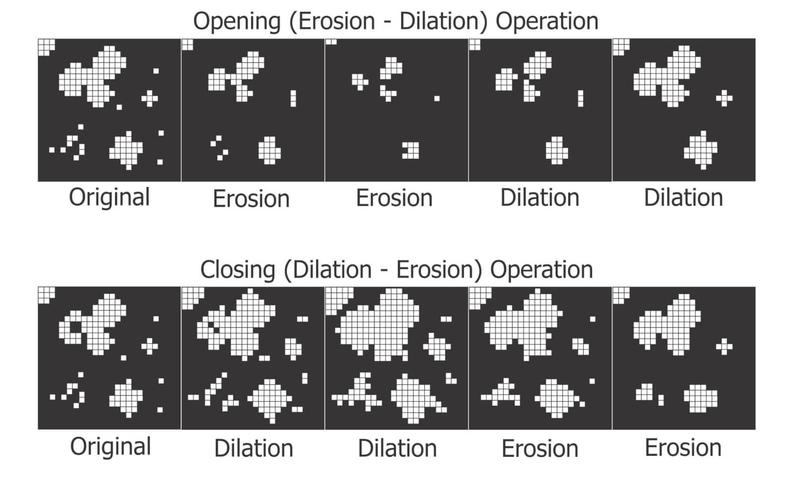
Many image processers use both these operations sequentially. When an image is eroded and then dilated (a process called “Opening”), smaller objects are removed, leaving the area and shape of remaining objects relatively intact. Dilating and then eroding (a process called “Closing”) fills in small holes and merges smaller objects, once again leaving the area and shape of remaining objects relatively intact. We can use both of these functions to help smooth an image prior to measurement.
(Top) Opening operations erode and then dilate the image. Moving left to right, the smaller objects tend to disappear. (Bottom) Closing operations dilate and then erode the image. Moving left to right, smaller objects either disappear or merge and holes are filled in
Distance Transformations
Distance transformations are advanced operations specifically used to separate objects that are densely packed. While not typically used when analyzing WSP, distance transformations are another means of identifying object nuclei. They are another means for teasing apart objects that are likely the result of overlapping deposits and then mapping their relative sizes and positions.
Measurement
The calculation of the area covered by deposits is straightforward. The pixels belonging to objects (the deposits) and those belonging to background are summed and then the fraction is converted to percent area covered. Research has shown that the image resolution does not significantly impact percent coverage assessments and has suggested that all image analysis software tends to produce similar results (+/- 3.5% observed when the same threshold was applied to multiple papers). This is acceptable because it’s within the variability inherent to spraying.
We ran a similar experiment wherein we analyzed the same piece of WSP using four methods. Here are a few facts about the software we used:
DropScope produces images between 2,100 and 2,300 DPI. Currently, it ignores ellipses and doesn’t count anything spanning less than ~35 µm (3 pixels).
We set ImageJ to ignore any object spanning less than 3 pixels, which at 2,400 DPI was 30 µm in diameter.
Snapcard was a free app created by Australia’s GRDC. It was benchmarked using ImageJ, tended to underestimate coverage and was fairly inconsistent. Nevertheless, it was convenient for field work. Instances may still exist, but as of 2025 it no longer available through the GRDC.
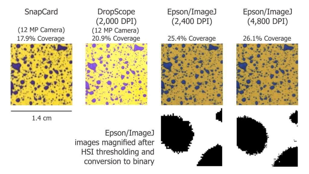
The images shown in the figure below were cropped from screenshots produced by each method. The actual ROI analyzed was ~3 cm2 for SnapCard, 3.68 cm2 for DropScope and 2.0 cm2 for both Epson/ImageJ methods. Our results indicate an +/- 4% difference in percent area coverage. This variability reflects the results of a 2016 journal article that compared SnapCard with ImageJ and other leading analytical software. That study claimed no statistically significant difference in percent coverage detected (standard deviations were about 20%). However, the ImageJ results tended to trend several percent higher than SnapCard. We saw this as well. And so, while resolution may not have a significant impact on percent area covered, there does appear to be some correlation.
Percent area covered as reported by three image analysis systems. Only a minor difference was observed when resolution was doubled using the Epson/ImageJ method.
Resolution definitely affects deposit counts. Particularly in applications that employ finer droplets. Consider the difference between detecting or missing 1,000 30 µm diameter objects. It may only amount to a fraction of a percentage of the surface covered, but +/- 1,000 objects on a 2 cm2 area is significant in terms of deposit density.
Output
Once a WSP image (or set of images) has been scanned, pre-processed, processed and measured, we will receive some manner of output. Some software packages create an attractive report with images, graphs and key values. These reports include percent coverage and many provide droplet density. Deposits may be binned by size, or spread factors are used to calculate the original droplet diameters and even estimate the volume applied by area. Other software packages provide raw data that can be imported into a statistical program or spreadsheet program like Excel for further analysis. Some software packages provide both.
How far can we take this?
Blow-by-blow data analysis is beyond the scope of this document, but how much weight should we give to coverage data obtained using WSP? The answer depends on the metric in question, but in all cases we must first acknowledge the three overriding caveats. Take it as said that they apply to everything that follows:
Different brands (and even different production runs) of WSP can produce significantly different coverage metrics. When conducting experiments, use a single brand of WSP. Better still, use papers from the same production batch whenever possible.
The same of piece of sprayed WSP can produce significantly different results depending on the software and protocol used to analyze it. When conducting experiments, use the same software and assessment protocol and be transparent about the process when communicating results.
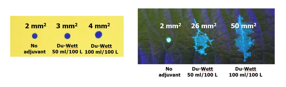
WSP coverage may not reflect the coverage achieved on an actual plant tissue surface. It is suitable as a relative index (I.e. papers can be compared to papers, but not to tissues) but the spread factor changes with surface wettability and the surface tension of the liquid sprayed. Note the differences in percent area covered in the following experiment with an organosilicone super-spreader:
Difference in deposit spread on water sensitive paper versus a leaf surface using an organosilicone super-spreader and UV dye. The same volume was applied in each case and while the area increased two-fold on WSP it increased ~10-fold on an actual leaf. Image reproduced from work by Robyn Gaskin, Plant Protection Products, New Zealand.
Recall that we started this document by listing the four pieces of information commonly sought using WSP. They were listed in order of reliability, and now we can explain why.
The percent surface area covered: We have established that this is the most reliable piece of data. Droplets do not spread on WSP the way they do on plant surfaces, so it will underestimate actual coverage. The results vary by analytical method, but it’s likely not dependent on resolution and still falls within the variability inherent to spraying. This metric gives us valuable and actionable information. We can say whether or not we hit a target, and evaluate whether a sprayer change resulted in more or less deposit.
The density of deposits on the target area: We have established that that there are limits to the reliability of this metric. It is affected by the analytical method used and can be greatly underestimated when resolution is poor or when deposits overlap in high numbers. Also, it will never reliably reflect deposits under 30 µm. Nevertheless, under controlled conditions this information does have value and is of great interest in enquiries about drift and contact fungicides.
The size of the droplets that left the stains: This metric is highly questionable except under controlled conditions. The many assumptions about surface tension, droplet speed, and droplet evaporation make it impossible to make definitive statements about spray quality. Finer droplets are greatly underestimated in this equation. Therefore, while there may be some value in using WSP as a relative index, this metric is a crude indication at best.
The dose applied to the target surface: This metric has not been discussed up to this point, but is quickly and easily dismissed. Let’s assume that a droplet with a high concentration of an active ingredient will leave a stain that is the same area as another droplet with a lower concentration. This will lead some to suggest that as long as the original concentration is known, we can back-calculate the dose (which is the amount of active on a given area). However, one droplet has the same volume as eight droplets that are half it’s diameter. This cubic relationship means that if they all deposit, the larger droplet will cover roughly 1/2 the surface area as the eight smaller droplets. Therefore, the smaller droplets spread the same amount of active over a greater area. Spread factor muddies this a bit, but ultimately it means that dose cannot be estimated from area covered. Dose is better assessed using collectors that permit the residue to be removed, such as Petri dishes, Mylar sheets, pipe cleaners, alpha cellulose cards, or glass slides.
And so, the image analysis process described here is powerful and effective when used with water sensitive paper as long as the limitations are acknowledged. The same process can also be used with dyes and specialized collectors such as Kromekote to permit even greater resolution. But that’s another story.
2026
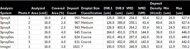
A new Brazilian cellphone-based system (SprayDex) emerged in 2026 that offers possibilities. Preliminary testing alongside other methods indicate it is consistent within itself, but as we saw in previous testing, the same WSP scanned using different systems will create different results. This is why, ultimately, WSP is a relative index and should only be compared within a given system; coverage cannot be reliably compared across WSP brands, or between digitization methods.
2026 Comparison of three digitization / analysis methods. Same WSP was scanned each time.
Marçal, A.R.S., Cunha, M. 2008. Image processing of artificial targets for automatic evaluation of spray targets. Trans. of the ASABE. 51(3): 811-821.
Moor, A., Langenakens, J., Vereecke, E., Jaeken, P., Lootens, P., Vandecasteele, P. 2000. Image analysis of water sensitive paper as a tool for the evaluation of spray distribution of orchard sprayers. Aspects of Applied Biology. 57.
Panneton, B. 2002. Image analysis of water‐sensitive cards for spray coverage experiments. Applied Eng. in Agric. 18(2): 179‐182.
Salyani, M., Zhu, H., Sweeb, R.D., Pai, N. 2013. Assessment of spray distribution with water-sensitive paper. Agric. Eng. Int.: CIGR Journal. 15(2): 101-111.
SnapCard website. University of Western Australia and the Department of Primary Industries and Regional Development, Western Australia. (Note: As of 2026, may no longer exist).
Syngenta. 2002. Water‐sensitive paper for monitoring spray distributions. CH‐4002. Basle, Switzerland: Syngenta Crop Protection.
Turner, C.R., Huntington, K.A. 1970. The use of a water sensitive dye for the detection and assessment of small spray droplets. J. Agric. Eng. Res. 15: 385-387.
Authors: T M Wolf, B C Caldwell and J L Pederson. Originally published in Aspects of Applied Biology 71, 2004, in expanded form.
Abstract
Spray drift deposition into water bodies may pose environmental and health hazards, and buffer zones have been suggested as a means of mitigating water contamination. Field trials were conducted to determine the effect of nozzle type and riparian vegetation on spray drift deposition into wetlands. Three riparian vegetative types, minimal vegetation (grass), low vegetation (willow shrubs), and high vegetation (aspen trees) were compared with open field conditions. Spray was released upwind of wetlands with these riparian characteristics with conventional and air-induced low-drift nozzles. Low-drift nozzles reduced drift deposits by about 75% in the absence of any vegetation, and by 88 to 99% when vegetation was present. Dense willow shrubs resulted in anomalous downwind deposits, possibly because of air turbulence caused by low porosity characteristics. By considering vegetation effects, a 15-m buffer zone could be reduced to 5 to 7 m for conventional, and 1 to 4 m for low-drift nozzles without increasing deposits at the edge of the sensitive habitat. Both variables should be considered by regulatory bodies in their risk assessment procedures.
Introduction
Airborne transport is an important vector for movement of pesticides from agricultural land to receiving waters. In an effort to maintain low pesticide levels in water bodies in accordance with risk assessment protocols, the Pest Management Regulatory Agency (PMRA) is mandating minimum setback distances (buffer zones) from water bodies during a spray operation. Several additional variables can complement buffer zones in preventing spray drift, including low-drift sprays and riparian vegetation. Germany and the United Kingdom already account for these characteristics in their buffer zone regulations (Kappel and Taylor, 2002).
Vegetation has been shown to be effective at mitigating droplet spray drift in several recent studies and reviews (Richardson et al., 2002, Hewitt, 2001, Ucar and Hall, 2001) by reducing wind velocities and intercepting spray. The documented magnitude of the spray drift deposit reduction in these studies ranges from 50 to >95%, dependent on variables that include vegetation height, porosity and orientation relative to wind direction, and wind speed.
We studied the integrated effect of buffer zones, vegetative barriers, and low-drift sprays to determine the overall impact of spray drift deposition onto downwind water bodies.
Materials and Methods
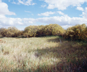
Overview and Site Description
The study was conducted in 2001 on a farm field near Aberdeen, SK. Sprays were applied upwind of a water body, and drift deposits were collected on petri-plates placed near ground level. Experimental sites were chosen to represent different vegetation heights and types around the water body in question: low (uncut grass), intermediate (willow shrubs), and tall (aspen trees). These were compared to nearby open-field conditions. Two sprayer nozzle types were used in the study: conventional flat fan nozzles and venturi-type low-drift nozzles.
The grass barrier was comprised of a mix of grasses dominated by bromegrass (Bromus spp.) growing to a height of 75 cm. Willows (Salix spp.) were approximately 3 m tall with a density of about 0.15 m-2 and presented a fully foliated barrier for their full height. Willows extended for a width of about 7 m toward the edge of the water body. Trembling aspen (Populus tremuloides Michx.) were approximately 8 m tall, with foliation beginning 1.5 m above ground. Trees were present at a density of about 0.25 m-2 and extended for 8 m toward the water edge.
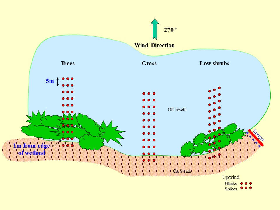
Figure 1: Site and sampler layout
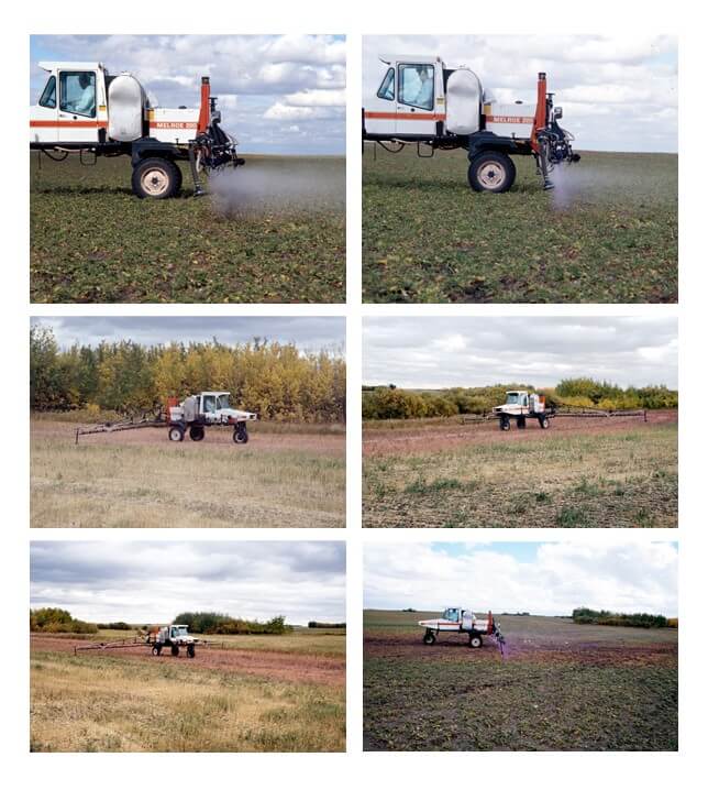
Spray Equipment and Application Method
A Melroe Spra-Coupe 220 was used to make the applications. This sprayer was equipped with conventional flat fan nozzles (XR8003) and air-induced low-drift nozzles (TD11003) at 275 kPa, producing ASABE Fine and Coarse sprays, respectively. The spray boom was 10 m wide and nozzles were 75 cm above ground. Sprayer travel speed was 12.9 km h-1, at which the application volume was 100 L ha-1.
The sprayer tank contained a mixture of 2,4-D amine4 (4 g L-1) and Rhodamine WT5 (2 mL L-1), a fluorescent tracer dye which would be used to quantify the deposits. 2,4‑D acted to photostabilize the dye, and also provided a spray formulation with physico-chemical properties representative of agricultural pesticides.
Top row: Fine and Coarse sprays used in study Middle row: Tall and medium vegetation Bottom row: Short vegetation and open field
Application was made in a direction approximately perpendicular to the prevailing wind, with the downwind edge of the spray boom at the edge of the wetland’s riparian vegetation. This was usually about 15 m upwind of the edge of the water body (due to severe drought conditions, the wetland did not contain any water at the time of the trials). Three consecutive passes were made along the same swath in a 10-min period to obtain average meteorological conditions for all three vegetation types. Wind speed and direction, temperature and relative humidity were monitored during application using a portable micrometeorological station.
Sampler Layout
Downwind of the spray swath there were 3 parallel lines of eleven 15-cm diameter glass petri-plate samplers starting underneath the sprayer boom and extending 46 m downwind from the edge of the spray swath (Figure 1). Samplers were separated by 5 m within the line, and lines were about 2 m apart.
The deposition profile was also assessed under open field conditions, using the same sampler layout but on crop land with no riparian vegetation. These are referred to as ‘bare soil, or ‘reference’ samplers in this report and served as a baseline to determine the impact of the riparian vegetation.
Sample Collection and Analysis
Sample collection began 5 minutes after spray application was complete (See Table 2 for trial times). Beginning with the furthest downwind locations, petri-plates were covered with a plastic lid, and placed into dark boxes. Spray deposits on the samplers were washed off in the laboratory using 95% ethanol in three 15-mL washes. Final samples were made up to 50 mL. and two 20-mL sub-samples were collected in borosilicate vials and stored in the dark.
Within 24 h, subsamples were analyzed using a fluorescence spectrophotometer with excitation and emission wavelengths of 545 and 570 nm, respectively (Shimadzu Model RF-1501 spectrofluorometer equipped with Model ASC-5 auto-sampler). Instrument readings were converted to µg L-1 using standard curves and expressed as a percent of the applied dosage under the field sprayer.
The fluorescence spectrophotometer data were averaged over the three replicate sampling lines, adjusted for photolysis, and expressed as a percentage of the amount applied on-swath. Relationships of spray drift deposits with downwind distance were first visualized by plotting all data points, and then mathematically related through appropriate regression techniques.
Results
Meteorological Conditions
Weather conditions were favourable during the trials. Wind speed and direction were appropriate for the sampler layout and the experimental objectives. Mean wind direction varied by up to 44º from the ideal (270º) in 6 out of 12 trials, and was within 30º for the remaining 6 trials (Table 1). Mean wind velocities were consistently between about 17 and 21 km h-1 in all but one trial. Air temperature and relative humidity fluctuated between 14 to 22º C and 31 to 80%, respectively, on the trial dates.
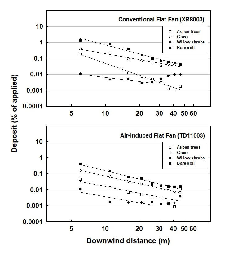
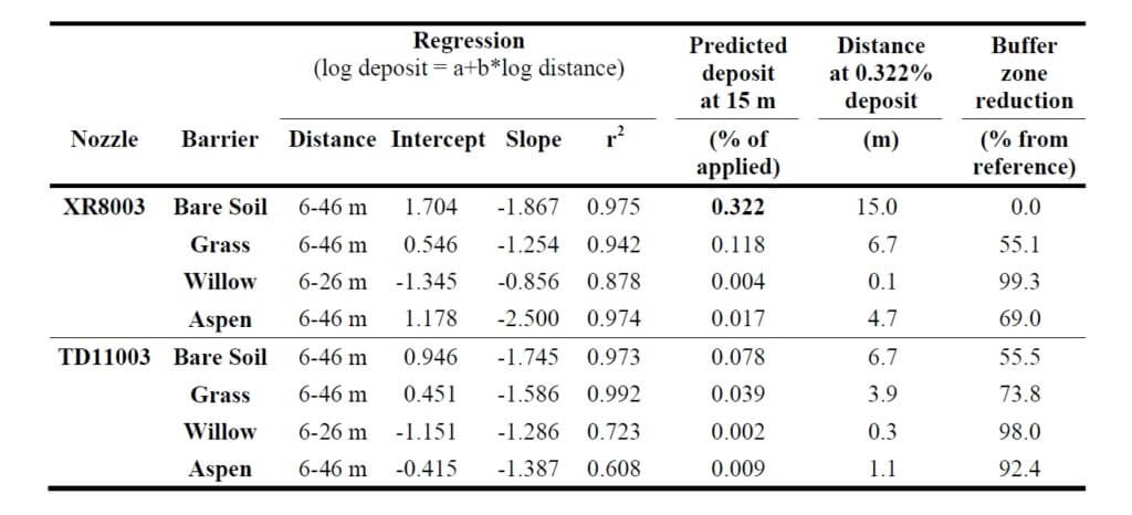
Deposition Profiles
A visual review of the raw data suggested that a linear regression of the log of deposit amount and log of downwind distance would be appropriate. It was noted that for willow, the deposit profile tailed upwards after the 26 m mark. Based on a survey of the site, it was concluded that this tail was probably caused by the length of the spray pass exceeding the length of protection offered by vegetation. In other words, beyond the 26 m sample, drift had not been attenuated by a vegetative barrier. It is also possible that the airflow was deflected up over the low, non-porous barrier and returned to ground level beyond the 26 m distance (Carter et al., 2001).
Figure 2: Spray deposit profiles from Fine (top) and Coarse (bottom) sprays. The deposition data for the willow were regressed from 6 to 26 m, all others were taken to 46 m (see text for explanation).
As a result of the questionable data for this vegetation type, it was decided that it would be misleading to include the furthest downwind data points. Implications of this observation will be discussed later in the manuscript. All regressions were statistically significant, explaining between 61 and 99% of the observed variation. In 5 of 8 trials, more than 90% of variation was explained.
Drift Mitigation by Riparian Vegetation and Application Method
The predicted drift deposit at 15 m was calculated for all trials based on the regression parameters (Table 3). For the conventional sprayer on bare soil, the deposit amount was 0.322% of the applied dose. The distance at which this specific deposit amount would be achieved was then calculated for all other trials. This value is the buffer zone distance at which equivalent protection to the reference system was offered. Buffer zones could therefore be reduced by 55% (grass), 99% (willow) and 69% (aspen) using the conventional nozzle and 56% (bare soil), 74% (grass), 98% (willow) and 92% (aspen) for the low-drift nozzle.
Table 1: Buffer zone distances based on observed drift, calculated from regression.
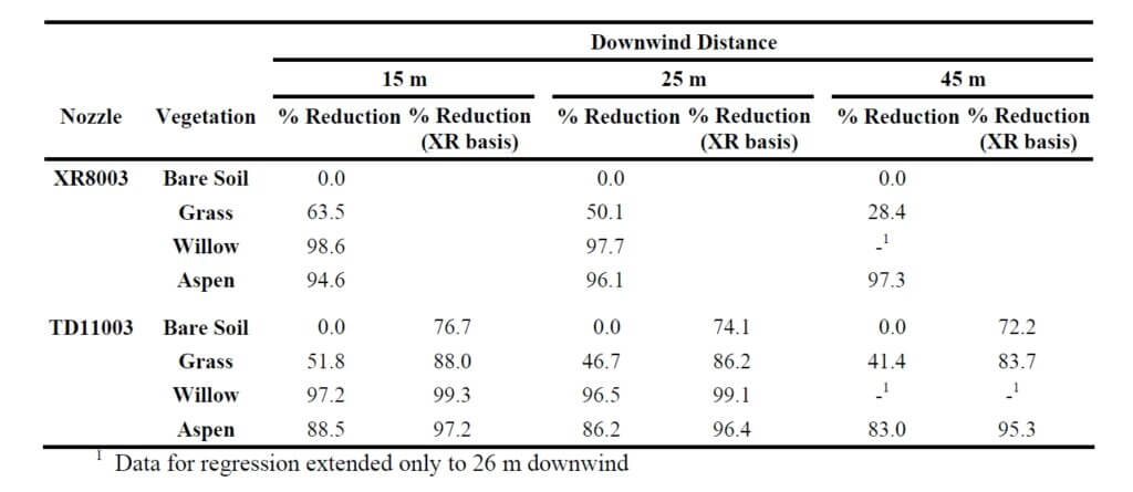
The calculated buffer zone reductions were not equivalent to the observed drift reductions due to the unique regression slopes of each deposition line. For example, expected drift deposits at 15 m downwind on bare soil were reduced by 77% when the air-induced low-drift nozzles were used (Table 4), whereas buffer zone distances could only be reduced by 56% (Table 3). Furthermore, the effectiveness of the grass vegetation diminished with distance, reducing drift by 64, 50, and 28% at distances of 15, 25, and 45 m, respectively. Therefore, a complete deposition profile will be required for each vegetation scenario to accurately adjust buffer zones.
Table 2: Drift deposits expressed as a percent of the reference deposition line for two application methods, four vegetation types, and three downwind distances. All numbers are the mean of three separate experiments on the same location.
Riparian vegetation was typically more effective than low-drift nozzles in protecting water bodies from drift deposition. While grass reduced deposition by 28 to 64% from the conventional nozzle (depending on the downwind distance), willow and aspen reduced deposition by between 95 and 99% (Table 4). The willow was not considered at further distances since the data used for the regression were truncated at 26 m. Low-drift sprays provided some additional protection in all cases except for trees at the 45 m distance, where deposits increased slightly relative to the conventional spray.
Discussion
The aerodynamics of vegetative barriers are a complex phenomenon. Wind, upon reaching a solid barrier, is diverted up and over giving strongly turbulent conditions on the leeward side and a rapid return to free wind speed. For a permeable barrier like a hedge, the return to free wind speed is more gradual since some air filters through, reducing the pressure differential and allowing for less turbulence (Davis et al., 1994). Wind speed reduction is most pronounced for a distance of 5 H upwind and 30 H downwind at the 1 H height, where H is the height of the barrier (Rider, 1951). Nonetheless, there may still be an upward diversion of air (and spray drift) which may simply delay, not eliminate, sedimentation (Hewitt, 2001, Ucar and Hall, 2001), particularly for dense hedges (Carter et al., 2001). Richardson et al. (2002) did not, however, notice such a deflection up to 10 m height.
The reduction in drift deposition by riparian vegetation in this study is clearly significant, but is subject to some interpretation. These data were generated at a single site, and while this site was carefully selected to be representative and trials were repeated three times, it does not necessarily constitute an average result. There are clearly any number of possible arrangements of trees, shrubs and grass, plus any additional vegetative or landscape features which would influence drift deposition behaviour. However, due to the consistent nature of the data of this study, some confidence is attained in that the numbers are at least reliable for the given set of conditions. In this study, three spray passes were made along the same swath at the edge of the water body. Results could have been different had adjacent spray swaths been used, owing to the possible change in contribution of upwind swaths with the altered airflows under vegetated conditions.
Since the water body was dry, additional grass vegetation which had grown up could have made an effective collector of spray drift, possibly reducing deposit values beyond those that would have occurred in a water body. It is recommended that efforts be made to repeat these studies when water is present at normal values.
The mitigating effect of vegetation depends on the aerodynamic features of the vegetation, as well as the collection efficiency of their leaves, twigs, etc. This poses some difficulties because there are no absolute measures of these features. Permeability, for example, varies with wind speed owing to the movement of leaves, and winds speed itself varies with height (Davis et al., 1994). Collection efficiency of the vegetation varies similarly with target size, its movement, wind speed, and droplet size spectrum (Hewitt, 2001). However, there are opportunities for improved characterization with specialized equipment, such as that used by Richardson et al. (2002). Their LIDAR instrument was able to help calculate tree height and width, mean area index and mean area density. Work to further characterize vegetation will prove useful in future efforts to understand its mitigating potential.
Low vegetation such as grass has not received the recent attention of hedges and trees but has also been documented to reduce spray drift significantly. A study by Miller et al. (2000) documented significant reductions in airborne drift concentrations above uncut grass canopies, even at low plant densities. Bache (1980) documented similar reductions in spray drift when sprays were applied over a mature wheat crop compared to bare soil. Therefore the filtering effects of “low” canopies may be very significant and should be the subject of further study.
Riparian areas are regions of high biological activity and diversity, not only protecting adjacent water from outside influence, but also providing food and shelter for many species of wildlife. These areas must themselves be protected from harmful effects, which can include pesticides. Their efficient capture of sprays suggests some risk from pesticides capable of controlling perennial vegetation. Likewise, pesticide residues in this vegetation have the potential to be ingested by wildlife or be washed off with precipitation, resulting in movement into the water body. These effects must be considered when using vegetation to mitigate airborne drift.
Conclusions and Recommendations
Vegetative barriers reduced spray drift deposition from conventional or low-drift nozzles into water bodies by 24 to 99%.
Low-drift sprays reduced deposition by about 75%.
Of the vegetation types, shrubs and trees had similar effects, reducing deposition from open-field conditions by an average of more than 95%. Low-drift sprays improved on this reduction.
Calculated buffer zone reductions were less than drift deposit reductions. Accurate determination of buffer zone distances requires that the entire deposition profile be characterized.
It is suggested that both riparian vegetation and sprayer technologies are important components of water body protection. Both should be considered in BMP and regulation development whenever the impact of pesticide applications near water bodies is to be estimated or mitigated.
Acknowledgements
The technical assistance of Glenda Howarth, Jill Clark, Rachel Buhler, Murray Nelson, Trevor Linford, and Pam Reynolds is greatly appreciated. Financial assistance was provided by the Rural Quality Program of the Agri-Food Innovation Fund, administered by the PFRA. The authors wish to thank Darrell Corkal and Clint Hilliard of PFRA for their enthusiasm, support and guidance directed towards this project, and Raymond Malko for making his land available for the trials.
Citations
Bache, D. H. 1980. Transport and capture processes within plant canopies. Spraying Systems for the 1980’s. BCPC Monograph No. 24, 127-132.
Carter, M. H., R. B. Brown, K. A. Bennett, M. Leunissen, V. S. Kallidumbil, and G. R. Stephenson. 2000. Methods for reducing buffer zone requirements for pesticide spraying adjacent to wetland environments. Sainte-Anne-de-Bellevue, Quebec: Proc. 2000 National Meeting, Expert Committee on Weeds / Comité d’experts en malherbologie [on-line: http://www.cwss-scm.ca/pdf/ECW2000Proceedings.pdf].
Davis, B. N. K, M. J. Brown, A. J. Frost, T. J. Yates, and R. A. Plant. 1994. The effects of hedges on spray deposition and on the biological impact of pesticide spray drift. Ecotoxicology and Environmental Safety 27:281-293.
Hewitt, A. J. 2001. Drift Filtration by natural and artificial collectors: a literature review. Special publication by Spray Drift Task Force, 12 pp. [on-line: http://www.agdrift.com]
Kappel, D. and W. A. Taylor. 2002. Buffer zones and “low drift” equipment. Hardi International Discussuion Paper, available from Hardi International A/S Helgeshøj Allé 38 DK-2630 Taastrup.
Miller, P. C. H, A. G. Lane, P. J. Walklate, and G. M. Richardson. 2000. The effect of plant structure on the drift of pesticides at field boundaries. Aspects of Applied Biology 57:75-82.
Richardson, G. M., P. J. Walklate, and D. E. Baker. 2002. Drift reduction characteristics of windbreaks. Aspects of Applied Biology 66:201-208.
Rider, N. E. 1951. The effect of a hedge on the flow of air. Quarterly Journal of the Royal Meteorological Society 78:97-101.
Ucar, T. and F. R. Hall. 2001. Windbreaks as a pesticide drift mitigation strategy: a review. Pest Management Science 57:663-675.
Wolf, T. M. 2000. Low-drift nozzle efficacy with respect to herbicide mode of action. Aspects of Applied Biology 57:29-34.