Drift symptoms can take a few weeks to be discovered, and to figure out the cause, people need to reconstruct the conditions during the application in question. Wind direction is the easiest. But when we consider factors like inversions, volatility, calm conditions, and others used to explain the movement of pesticides, it can quickly become quite confusing.
Let’s review how and why pesticides move.
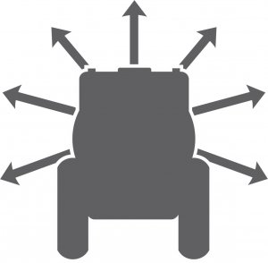
There are about six main ways that pesticides can move off-target.
- Droplet drift at the time of application;
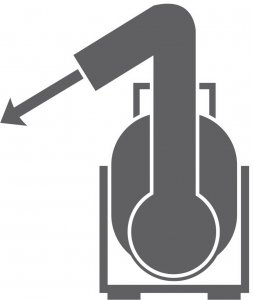
- Vapour drift at or after the time of application;
- Pesticide movement in water (precipitation or runoff) after application;
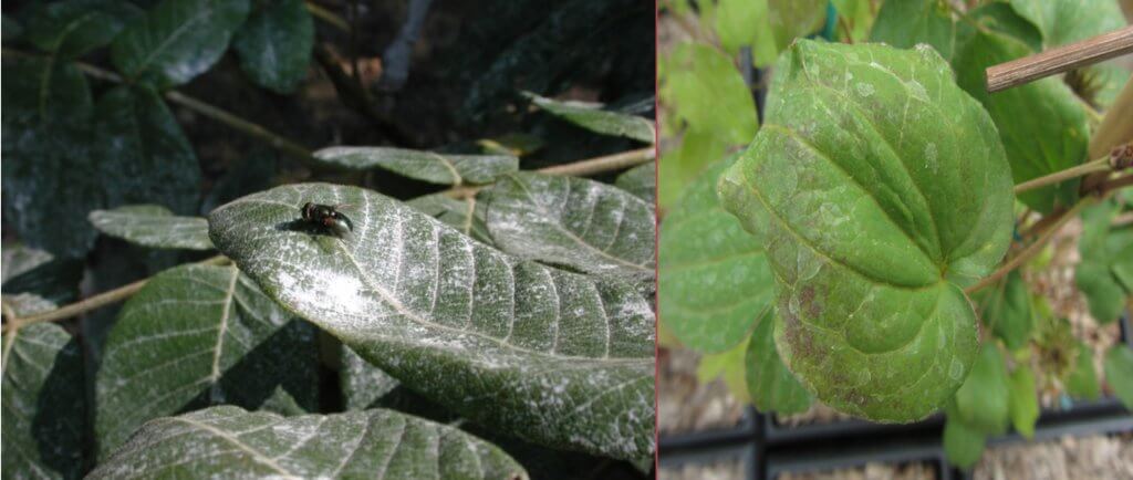
- Dislodgeable residues from plant surfaces after application;
- Pesticide-containing soil movement after application;
- Pesticide residue in sprayers applied to another site.
Whenever we find pesticides in a place where they do not belong, usually first indicated by plant symptoms specific to that herbicide, we need to find out the possible reasons and take steps to prevent that from happening again. We’ll focus on the first two items from the above list because those two are the most common.
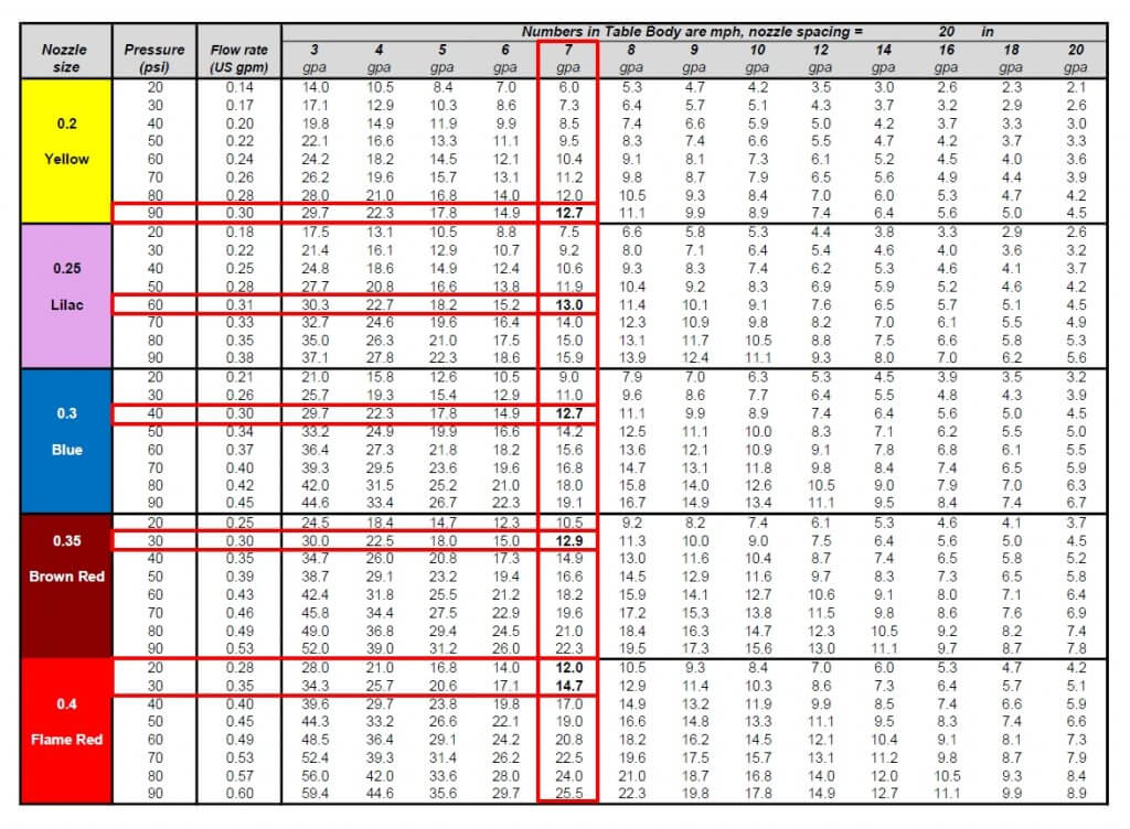
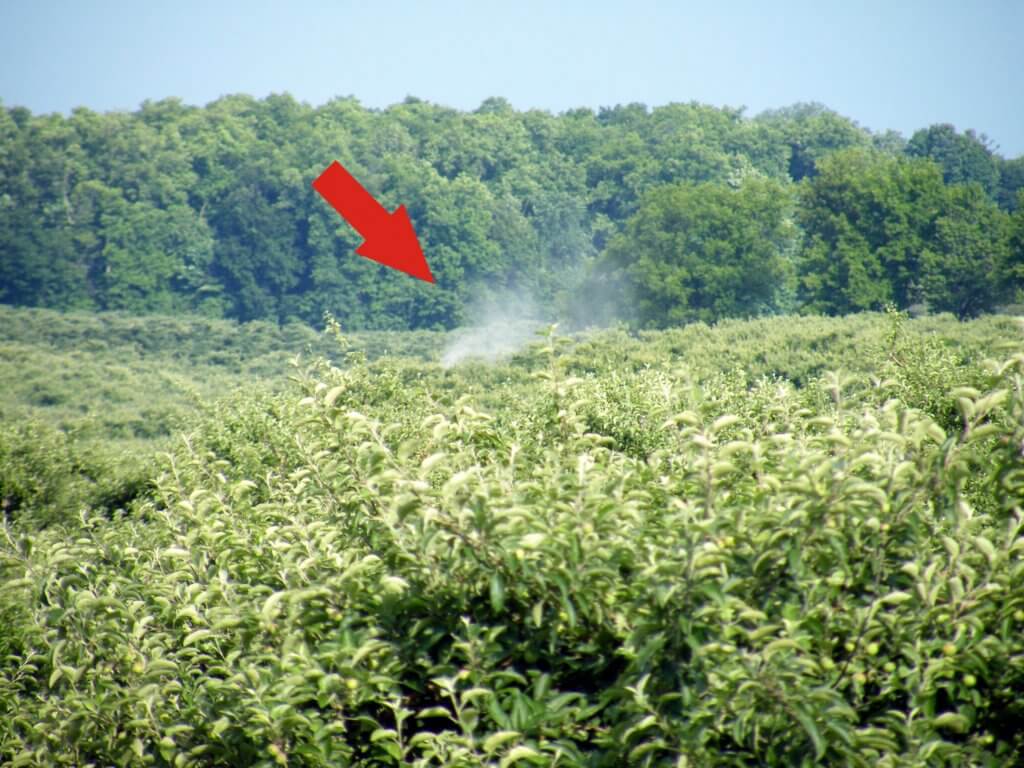
Droplet Drift: Sprayer nozzles produce droplet sizes ranging from 5 to 1000 µm, some up to 2500 µm. All nozzles, even the venerable low-drift tips recommended for dicamba application, will have a fraction of their volume in driftable droplets, say, less than 150 to 200 µm. For the low-drift sprays, that fraction is indeed very low, only a few percent of the total spray volume. For conventional nozzles, the driftable fraction may be 10 to 20% or more if high pressures are used.
Tiny droplets have no energy of their own and move with the air mass they’re released into. If it’s windy, they move downwind. If the air is turbulent, they move up and down. If the atmosphere is stable, the buoyant fraction stays aloft and concentrated. So in order to understand their movement, we need to understand the atmosphere.
Vapour Drift: Some chemicals are inherently volatile. This means they convert from the liquid or solid phase to a vapour phase on their own in accordance with temperature. Water is a great example, it is highly volatile. It is also able to sublimate, which means it can convert from a solid directly to a vapour without going through the liquid phase. An example of that is freezer burn, in which ice cubes shrink due to water escaping as a vapour.
Volatile pesticides can also sublimate. On landing on a leaf or soil, a significant portion of a droplet is absorbed or adsorbed. Some fraction may dry on the leaf surface. This remaining solid can volatilize (form a vapour) for hours or days after application. The rate of evaporation is driven by two factors, (a) the background vapour pressure of the substance in the atmosphere, and (b) the surface temperature of the object the chemical is resting on. For water, the atmospheric vapour pressure can be expressed as relative humidity. Droplets evaporate slower when the atmosphere is already full of water.
Pesticide evaporation is driven primarily by surface temperature. The background concentration of pesticide in the air is much lower than saturation, and has no effect. Pesticide evaporation is not directly affected by relative humidity because vapour pressures are independent of each other. In other words, most active ingredients will evaporate at the same rate whether the RH is 30% or 100% (it’s actually a bit more complicated than that. See the Note on Evaporation at the bottom of this article). This will be on the test, kids.
Vapour losses can be minimized by choosing low-volatile pesticides and also by making the application on cooler days. We also need to watch the forecast and avoid spraying when tomorrow or the day after is forecast to be hot.
Sometimes a rainfall can affect vapour losses, prompting a release of pesticide into the atmosphere. This behaviour can be predicted by the Henry’s Law Constant of a chemical.
Inversions: There are two types of turbulence, mechanical and thermal. Mechanical turbulence results from air encountering friction as it moves across a landscape. Taller objects and stronger winds result in greater mechanical turbulence. This turbulence creates small eddies that allow different layers of the atmosphere to communicate with each other and transfer momentum and contents up and down. More mechanical turbulence means more mixing and more sedimentation and dilution of a contaminant. In other words, the downwind impact of drift particles is reduced with greater mechanical turbulence. Mechanical turbulence happens whenever it’s windy, day or night, and it tends to counteract thermal turbulence.
Thermal turbulence is more powerful than mechanical turbulence for dispersion of pollutants. Driven by the solar heating of the earth’s surface, that causes the lower atmosphere to be much warmer than the air higher up. The atmosphere normally cools the higher you go (at about 1°C/100 m, called the dry adiabatic lapse rate), but when it’s sunny, the gradient is greater. In other words, it cools faster because the air at the ground is warmer.
Thermal effects move large parcels of air up and down, and we call this an unstable or a turbulent atmosphere. When parcels of air rise and fall great distances, we get a powerful diluting effect which is usually associated with a breeze but can also happen under calm conditions. An unstable atmosphere is great at dispersing drift, minimizing its downwind impact. This can only happen during the daytime, is most powerful when it’s sunny, and almost never happens at night.
By the way, a neutral atmosphere occurs when the rate of air cooling with height equals the adiabatic lapse rate described above. A neutral atmosphere can occur on cloudy days just before a rain, or on windy nights. There are no thermal effects in a neutral atmosphere, and the only dispersion occurs due to mechanical turbulence (windy conditions).
A stable atmosphere (inversion) happens when there is no solar heating of the soil. In other words, it can only happen when the sun is low in the sky or at night. In this case, soil cools off and the cold soil cools air near it. As a result, the air temperature rises with elevation. Since it’s normal for air to cool with elevation (at the dry adiabatic laps rate mentioned earlier), the temperature profile is now…inverted. Hence the name “inversion”. To be clear (write this down kids, it’s on the test), an inversion describes an atmospheric condition in which (potential) temperature rises with elevation. That’s it. It rarely happens during the day, but is common on clear calm nights. (btw, “potential temperature is the temperature adjusted by its normal rate of cooling with height. To have thermal effects, the rate of cooling needs to be different from this rate.)
The atmosphere is called stable because there is no thermal mixing. Air parcels stay put. Suspended particles such as tiny droplets stay put. Drift clouds stay concentrated, potent. If you make a fire, smoke hangs around. Cool, dense air is near the ground, and moves laterally very slowly, and might run downhill, like water, in a sloped setting. This situation is dangerous because it can move pesticide particles or vapours great distances without them becoming diluted or dispersed. An additional danger is that relative humidity is higher at night, delaying evaporation of water from the droplets. They stay potent.
In Summary: Pesticides move in the atmosphere and are rapidly diluted by mechanical, and especially thermal, turbulence. That is why we like to see spray applications on sunny days with a nice breeze, which moves the product in a predictable direction and dilutes any drift rapidly along the way. We minimize particle drift through the usual measures such as the use of low booms, protective shields, slow travel speeds, and coarser sprays. We avoid spray application of volatile pesticides on or preceding hot days to minimize the risk of vapour drift. We do not apply pesticides when the atmosphere is stable (inversion), which usually means from just before sunset to just after dawn on a clear night.
OK, that’s the basics. Now let’s explore some common questions.
- Can all pesticides move as particles and vapours? All pesticides that are atomized through a nozzle can move as particles. Only pesticides that are considered “volatile” can form significant amounts of vapour and move in that form. Dicamba is volatile. New dicamba formulations such as Xtendimax, FeXapan, and Engenia are much less volatile than older formulations, but they’re still capable of moving as vapours. Glyphosate and many other pesticides are not considered volatile and are not known to cause vapour drift.
- Are inversions only a problem for dicamba? Inversions affect droplet drift from all pesticides equally. The key difference is the amount of harm that any given droplet or vapour cloud can impart. Dicamba can harm conventional soybeans, many vegetable crops, and many trees and shrubs at extremely low doses. That means that even a weak inversion or a small amount of drift can cause great harm for long distances. In comparison, most other products are not as harmful to most of our crops in such small doses (I’m generalizing, forgive me). Tiny amounts may never be noticed, but they are there. Dicamba lets us notice these tiny amounts.
- Does vapour drift move only by inversions? No, although its movement is more damaging under inversions. Vapour drift clouds form above a recently sprayed canopy on hot days when leaf or soil surfaces contain a volatile product. On a sunny day (no inversion), this vapour will likely disperse rapidly downwind, causing diminishing damage with increased distance in relation to the sensitivity of the non-target plant. But towards evening, the dispersion (caused by thermal turbulence) ends as the sun sets and the atmosphere becomes stable. Now, the residual vapour cloud above the crop is no longer diluted, and may move in an unpredictable direction based on the slope of the land or a very gentle evening breeze. This movement may be significant, extending for miles in some cases, and potentially causing harm along the way.
- How long after application can vapour drift occur? Under most conditions, vapour losses diminish rapidly and will likely be gone within a few days as the pesticide is taken up by plants, metabolized, converted to a non-volatile form, etc. For some products, a light rainfall event can release a new wave of vapour drift because these products would rather be vapours than be dissolved in water, in accordance with their Henry’s Law Constant.
- Do some products drift further than others? Yes and no, but mostly no. Spray drift is a physical process governed by the behaviour of droplets in the atmosphere. Droplet diameter determines its mass and this mass controls the time it takes the droplet to sediment to the ground. The substance dissolved or suspended in that droplet has no bearing on this behaviour. But there are two key exceptions to consider. First, we know that some formulations generate more fine droplets than others even when atomized through the same nozzles. The greater abundance of small droplets will create more drift damage at any given distance, and also extend further downwind. And secondly, some formulations change the rate of water evaporation from the droplets. As a result, droplets moving downwind may shrink faster, in effect making them more drift prone and causing them to move further downwind. The same droplet size drifts the same distance, but droplet size changes. Question for the final: If you spray dicamba and glyphosate on the same day using the same nozzle, and the formulation has no impact on droplet size or evaporation, which one drifts further over a soybean crop? The answer is at the bottom of this article.
- Do calm conditions indicate an inversion? Inversions are defined as a temperature profile, not a wind condition. But the two are associated. An inversion is most pronounced and persists the longest under calm conditions, and because it suppresses atmospheric mixing, an inversion does prevent a windier upper atmosphere from reaching the ground. But it can be calm in the middle of the day with an unstable atmosphere. The calm condition eliminates mechanical turbulence, and therefore reduces the dispersion of the spray cloud. Calm conditions are also undesirable because the winds that follow a calm period are often unpredictable in direction, force, or duration. So it’s not a great idea to spray when it’s completely calm, even on a sunny day.
- Can inversions occur during the day? Yes, but it’s rare. Sometimes a large cold air mass moves into an area, say from a cool body of water, pushing warm air above it. So technically the air at the ground is cooler than the air above it, suppressing dispersion through that cap. Another situation is an inversion layer that forms at the top of a transpiring plant canopy. The air at ground level is warm, and cools suddenly where the crop evaporates water from its leaves. Air temperature rises with elevation above this transpiring layer, then cools again in accordance with an expected profile. So we have a thin layer in which vertical mixing is suppressed. This is most common in dense, thick canopies with adequate soil moisture on hot days.
- Is there an inversion every night? No. Cloud cover suppresses the rapid cooling of the soil, and the air at soil level stays warmer longer. Wind mixes the cold air layer into a warmer air layer, returning a more neutral condition. Inversions are most likely on clear nights with little wind. Recent data in inversion frequency from Missouri and North Dakota shows that inversions occur on the majority of nights, but the frequency depends on the location.
- Can drift be eliminated? Yes, we can eliminate spray drift by atomizing the spray in droplets (or, for dry soil-active products on carrier particles) large enough to resist movement in wind. We would need to be sure that absolutely no fine droplets or particles are produced, and that they don’t dislodge after application. That will require different atomizers and significantly more water volume and possibly new adjuvants. Some will argue that drift can also be eliminated by protecting the fine droplets with shields or air assist, but again, the protection would need to be 100%. Drift control has not been a high enough priority for these technologies to be developed and made available to applicators. Vapour drift can be eliminated by not applying volatile products.
Pesticide movement in the atmosphere is complicated. But pesticides don’t just move as a result of vapour or droplet drift. Consider all the options when investigating an affected field. And let’s all work together to better understand pesticide movement and to prevent it.
Answer: Both drift equally. But assuming the beans are susceptible to both herbicides, the dicamba damage will appear further downwind due to the greater sensitivity of the beans to this herbicide. This does not mean it drifted further.
Note on Evaporation: There is some discussion about the role of relative humidity on vapour loss. Although we stated that RH plays no direct role in pesticide volatility, we need to qualify that.
(a) Many pesticides dissolve in water. More water moves to plant or soil surfaces during periods of low RH, and this can carry dissolved pesticide with it. The supply of pesticide that can evaporate is thereby replenished.
(b) Evaporation is driven by temperature and the concentration gradient between the source and the atmosphere. In still air, the air layers closest to the evaporating surface are most concentrated with evaporated pesticide, slowing further evaporation. Air movement will remove these layers, increasing the rate of evaporation.
(c) co-distillation may occur for some pesticides. This means that the pesticide dissolved in water may evaporate with water, liberating it into the atmosphere. When co-distillation occurs, low RH would increase pesticide losses as well.
We still have much to learn about these phenomena, especially as it affects new formulations.