Category: Nozzles and Droplets

For Basics Category

  • What is Spray Quality, Part 4 – An Important Change in S572.3 and ISO25358

    What is Spray Quality, Part 4 – An Important Change in S572.3 and ISO25358

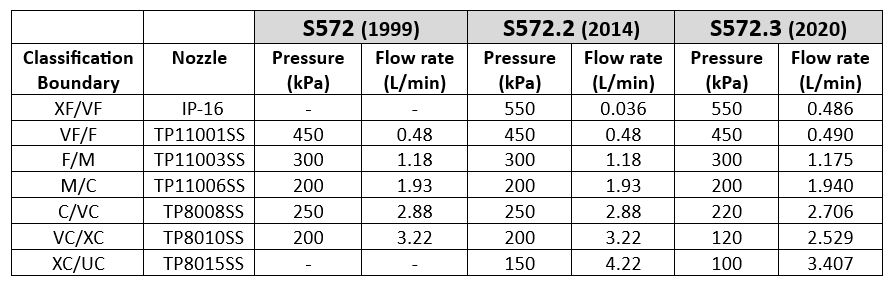
    A new version of standard ASABE S572.3 (adopted 2020) and its international equivalent, ISO 25358 (adopted 2018) addresses a limitation of the previous standards. In ASABE S572.2, the nozzle that defined the category boundary between the XC and UC sprays was the TP8015 SS at 4.22 L/min, corresponding to 150 kPa. Only very few nozzles produced UC sprays, and those that did only did so at the lower pressures and higher flow rates. For those nozzles, the categories worked.

    The emergence of a host of new low-drift nozzles designed to meet the regulatory requirement for drift protection for Xtendimax and other dicamba formulations in soybeans revealed the limitation of this boundary nozzle choice. In essence, all the new dicamba-compliant low drift sprays were UC, regardless of nominal flow rate or spray pressure. Any effect of, say, higher pressure that would create a finer spray, was not revealed. It was decided that new boundary nozzles were needed so that the coarser sprays’ response to flow rate, pressure, and formulation or adjuvant choice, could be better described.

    S572.3 therefore lowered the defining flow rate of the XC/UC nozzle from 4.22 to 3.41 L/min, with a new spray pressure of 100 kPa (from 150 kPa). This made the new boundary spray coarser. Because this change made the adjacent spray quality class, the XC, broader, the VC and C categories were each also widened somewhat, by lowering their respective boundary nozzle flow rates and pressures (Table 1).  

    Table 1: Change in spray pressure of three coarsest boundary nozzles from ASABE S572.2 to S572.3
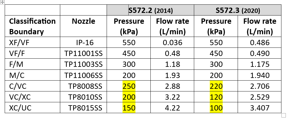
    For XF, VF, F, and M spray classes, there is no change with this new standard because the boundary nozzle conditions were not changed. But the C, VC, XC, and UC classes became coarser.

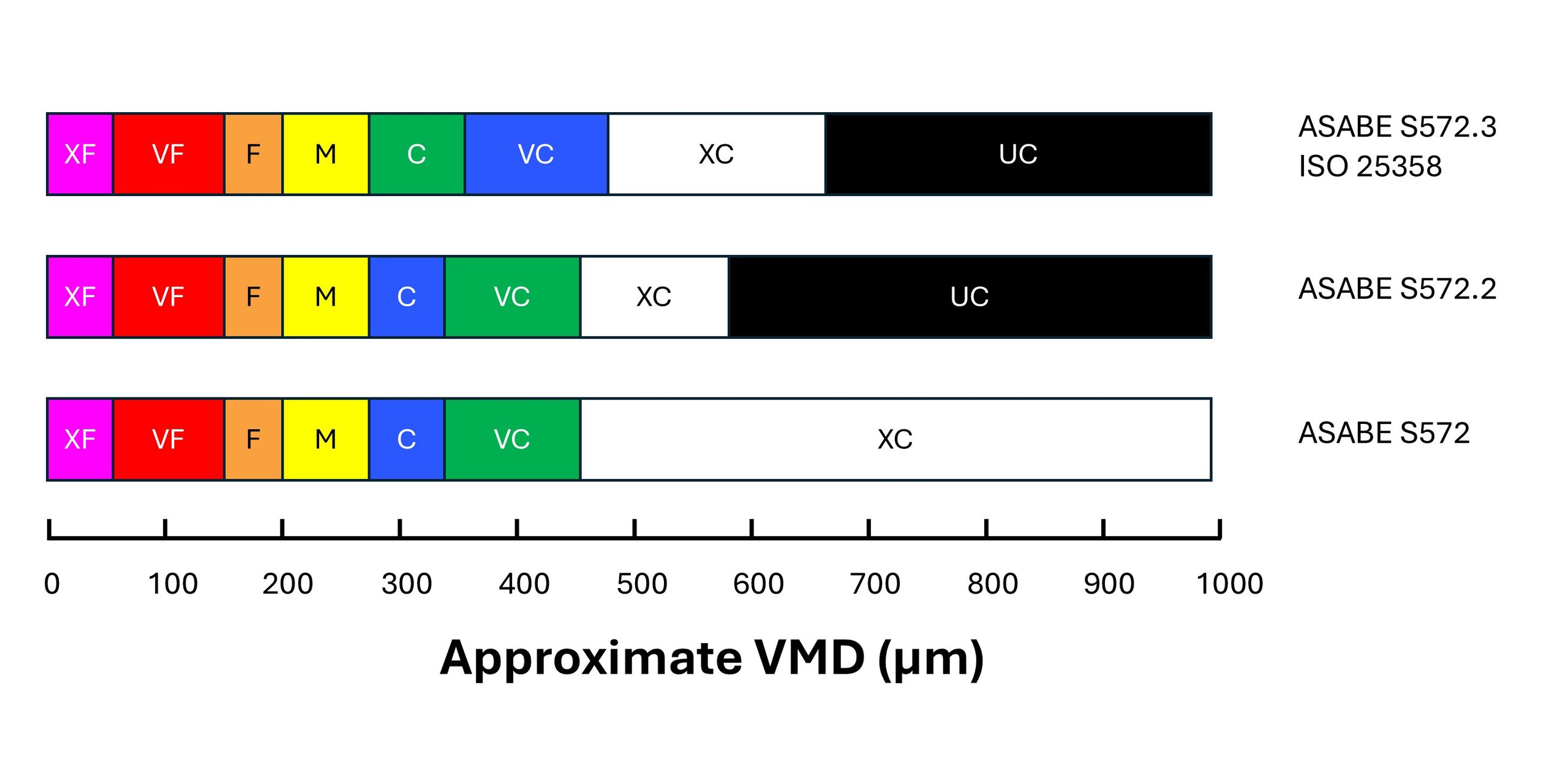
    In order to signal the change to consumers, the colour coding of the Coarse and Very Coarse sprays was switched. With S572.2, C was blue and VC was green. With S572.3, C is now green and VC is blue (Figure 1). 
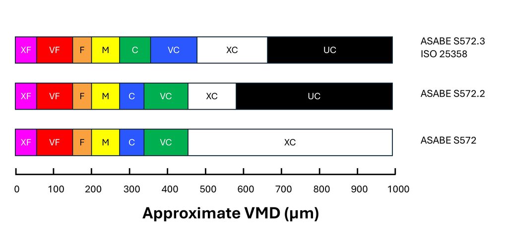
    Figure 1: Approximate changes in the Volume Median Diameter (VMD) of boundary nozzles under the S572 standard versions. Note that the coarsest spray quality categories are more equally distributed in the newest standard versions.

    The change means that low-drift sprays categorized using S572.2 can no longer be accurately compared to nozzles categorized using S572.3. For example, if a researcher conducted efficacy studies and concluded that ASABE S572.2 Coarse sprays provided acceptable efficacy, but S572.2 Very Coarse sprays had lower performance, they might recommend Coarse sprays. But would that recommendation be safe for nozzles classified with S572.3? In that standard, the C category extends into the territory formerly occupied by VC, deemed too coarse by the research.

    A similar problem exists for spray drift risk assessments. Let’s say a regulator recommends a 25 m buffer zone for ASABE S572.2 VC sprays based on modelling the drift from that C/VC boundary nozzle. What will the buffer zone be for the new S572.3 VC spray? Since the newer VC spray is coarser at its lower boundary, drift, and therefore the buffer zone, would be less. Determining how much so would require a new spray drift dataset for the new boundary nozzle.

    In fairness, most of the risk assessments are done on finer sprays such as Medium and Coarse, and those would remain unchanged because to be conservative, the regulator would assume the finest spray within each category (i.e., the lower boundary nozzle). But when a registrant requests that risk assessment be done with a coarser spray quality such as VC, XC, or UC, the regulator would need a new dataset.

    Another problem is that not all spray quality data reported by manufacturers use the new standard. Of the major North American manufacturers, Spraying Systems started reporting their products using the S572.3 standard in 2023. Pentair Hypro, and by extension John Deere, as well as Wilger Industries have not yet followed suit.

    The European manufacturers are well on their way. Lechler and Arag are both reporting using ISO 25358. But Agrotop and Billericay Farm Systems (BFS) are still reporting using the older standard.

    It may have been some years since nozzle manufacturers last tested the spray quality of their nozzles. If they now measure their sprays using the new standard, some other changes have also have ocurred in the interim. For example, new laser measurement systems may have been acquired. New scanning techniques may have been developed. New staff are operating the systems. And while the ASABE and ISO reference nozzles are intended to negate these differences, we are still seeing some discrepancies. It is also possible that changes to the manufacturing of the nozzles has also altered the spray quality they produce.

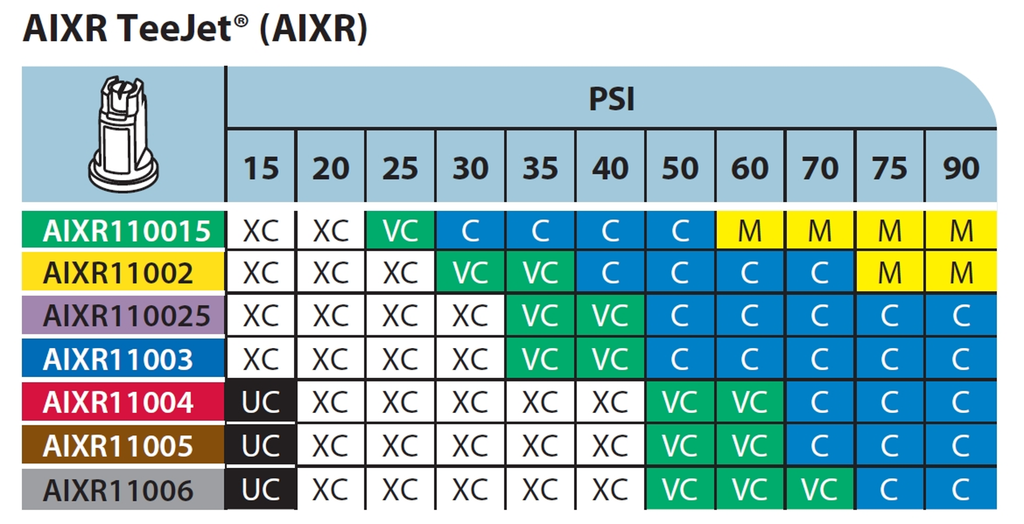
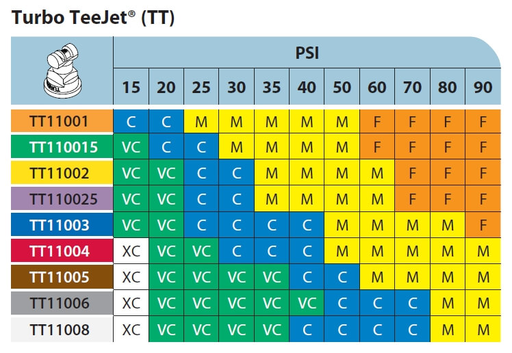
    For example, compare Figure 2, the TeeJet AIXR nozzle spray quality chart, developed using ASABE S572.2 and published in 2015, to Figure 3, the same nozzle whose spray quality was categorized using ASABE S572.3 and published in 2023.
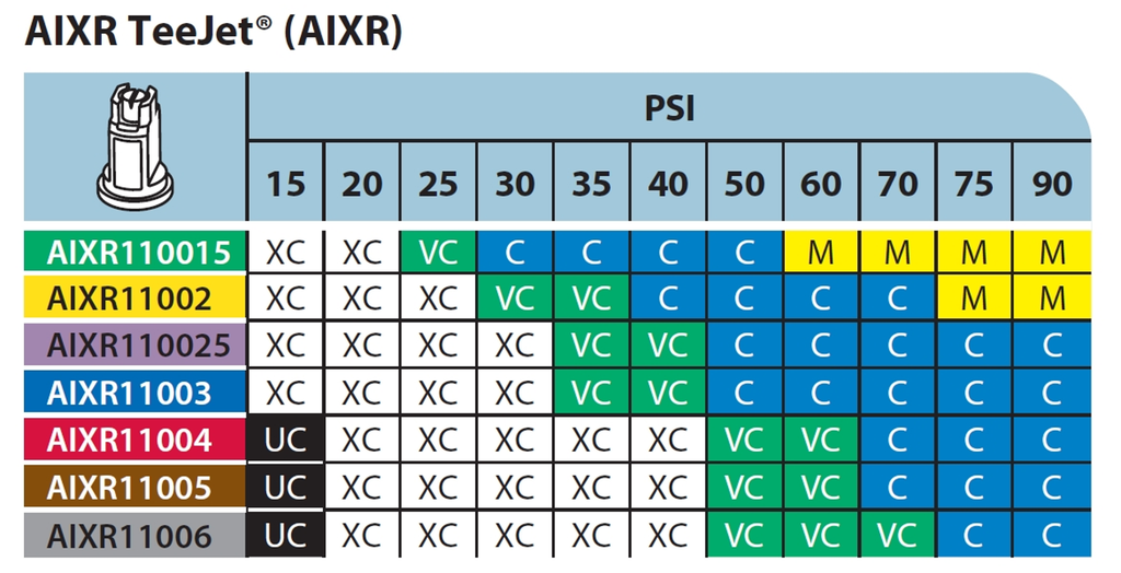
    Figure 2: Spray quality of TeeJet AIXR tips according to S572.2, published by Spraying Systems in 2015. Reproduced from TeeJet Catalog 51A.

    First, let’s compare the portion of the chart that reports Medium spray qualities in Figure 2 to that in Figure 3. These should be the same given that the same boundary nozzle and pressure was used in both. But under the new testing, the region reporting a Medium spray has significantly expanded towards the lower pressures. The Medium sprays begin at 60 and 75 psi in the old standard, but at 50 psi for the new standard.
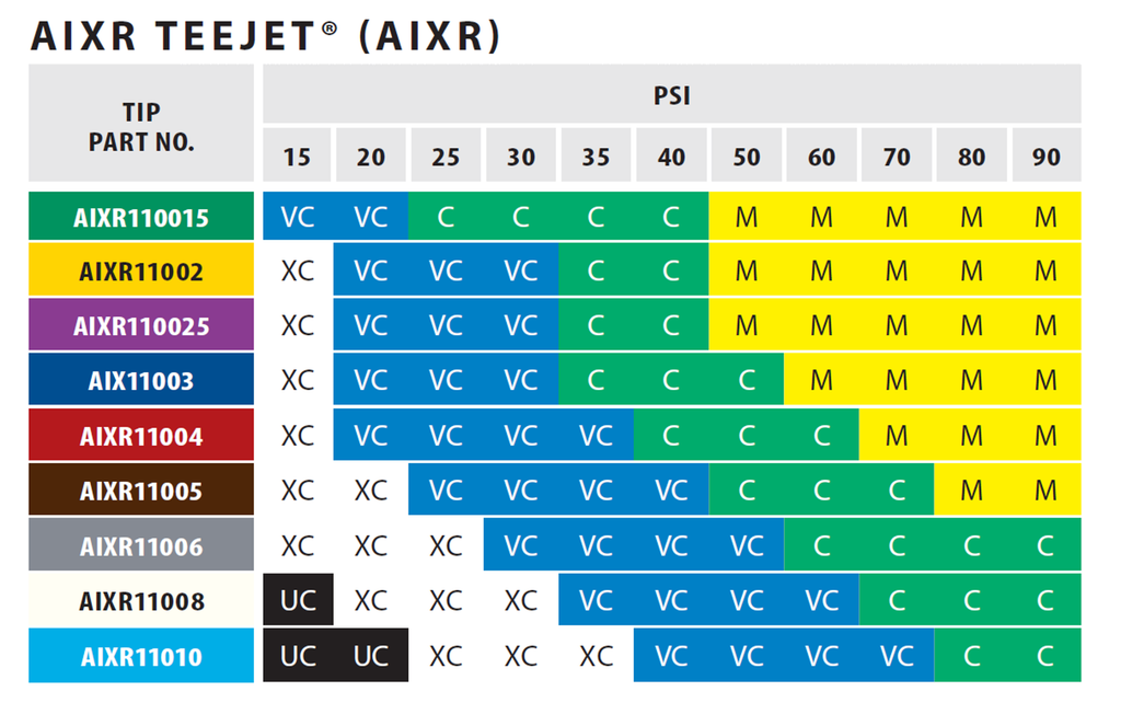
    Spray quality of TeeJet AIXR tips according to S572.3, published by Spraying Systems in 2023. Reproduced from TeeJet Catalog 52.

    The region occupied by the Coarse category has shifted towards lower pressures, as expected with the coarser upper (C/VC) boundary nozzle. It would be wider, as was the intent, had the M catergory not encroached.

    The region occupied by VC and XC have grown towards the lower left, more or less as expected. The VC category in particular, now dominates in the lower pressure region, a space previously occupied by the XC category. The small region which the UC category occupied under S572.2 in Figure 7 was replaced entirely by the XC category.

    Looking at it another way, the commonly used AIXR11004 size at pressures between 30 and 90 psi would have produced XC, VC, and C spray qualities in the old catalogue. The same nozzle now apparently produces VC, C, and M sprays at the same pressure range.

    These changes may or may not extend across all nozzles and manufacturers to the same extent as this example illustrates. But they add another level of complexity, and perhaps confusion, to applicators striving to be compliant with label directions. I am hopeful that the sector can quickly move to adopt the changes universally so that the mixed messaging is short lived and mistakes are minimized.  

    In particular, the regulatory bodies that rely on these spray quality classes to communicate drift potential and buffer zones must recognize that their risk assessments will need to reflect these new standards as more nozzle manufacturers begin communicating them.

    Droplet size continues to explain most of what matters in spraying, from deposition uniformity, to coverage and spray drift. Hopefully this series of articles explaining the measurement of spray droplet sizes is useful and sheds some light on how the industry measures and communicates it.
  • What is Spray Quality, Part 3 – The Evolution of Standards

    What is Spray Quality, Part 3 – The Evolution of Standards

    When scientists with laser droplet sizing instruments compared their results with other labs using the same nozzles, the numbers didn’t agree exactly. Laser equipment type and age, optics, operating settings, scanning techniques, and software versions were important. Everybody had their own numbers that they trusted more than their colleagues’ in another lab. In order to communicate droplet sizes to the end user consistently, a way to resolve these differences needed to be found.

    Scientists ushered in a new approach, that of using reference nozzles.

    Rather than argue about whose instrument or measurement method was correct, experts decided to allow each lab to use their equipment but with measurement protocols that met certain standards for scanning accuracy. The way the systems were compared was with a set of agreed-on reference nozzles. These reference nozzles defined the boundaries of spray qualities and were measured by the lab at the same time they tested other nozzles. When a nozzle of interest produced a spray whose parameters fell between two reference nozzles, the spray quality was thus defined. In this way, the peculiar results of a certain measurement approach became irrelevant. All that mattered was where the result lay with respect to the reference nozzles tested by the same lab.

    Credit is due to members of the British Crop Protection Council, who pioneered this result in the UK in the mid 1980s, and on which today’s droplet size classification standards are based. Their initial standard was first proposed in this paper:

    Doble S J, Matthews G A, Rutherford 1, Southcombe E S E (1985). A System for Classifying Hydraulic and Other Atomizers Into Categories of Spray Quality. Proceedings British Crop Protection Conference – Weeds, 3, 1125-1133.

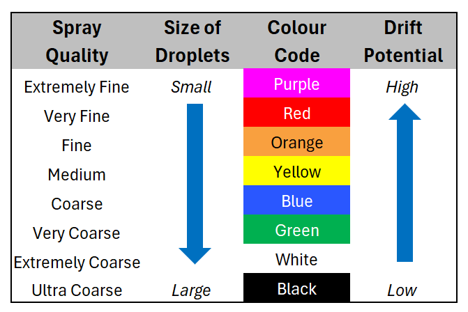
    Thus the term “Spray Quality” was born, and after various incremental revisions, sprays were named Extremely Fine, Very Fine, Medium, Coarse, Very Coarse, Extremely Coarse, and Ultra Coarse and given a colour code for easy identification.

    The American Society of Agricultural and Biological Engineers (ASABE) published the first Spray Quality Standard, S572, in 1999. It specified reference nozzles that formed boundaries from VF/F to VC/XC. It was updated to S572.2 in 2014 with the addition of the Ultra-Coarse category.

    Figure 1: Symbols and colours used to designate spray qualities according to ASABE S572.1 and S572.2

    In order to better represent nozzles that produced finer and coarser sprays, boundary nozzles for XF/VF and XC/UC were introduced with ASABE S572.1 in 2004. ASABE S572.2 corrected an error in the flow rate of the XC/UC in 2014.

    In 2020, ASABE S572.3 was introduced, following on the heels of ISO 25358 that changed the operating conditions for the C/VC, CV/XC, and XC/UC boundary nozzles.  S572.3 and ISO 25358 share the same boundary nozzles, allowing for similar implementation of the spray qualities across borders.

    Table 1: ASABE S572 spray quality categories and their respective boundary nozzles and operating parameters.

    The newest standards changed the boundary nozzle conditions for C/VC, VC/XC, and XC/UC as shown in Table 1. This was done in order to create more equally sized spray quality categories for the coarsest sprays.

    How the Standard is Implemented

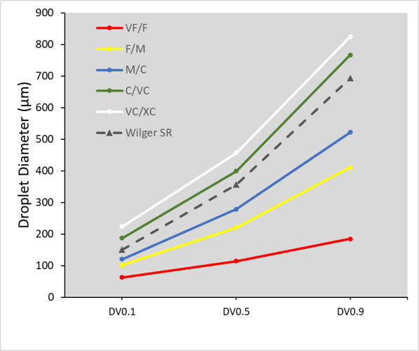
    A laboratory that measures spray qualities would start by running the ASABE reference nozzles on their instrument. They would then calculate the three parameters we described in Part 2 (DV0.1, DV0.5, and DV0.9) and plot them as shown in Figure 2. Next, the lab would atomize various nozzles, pressures, adjuvants, etc. of interest to see where their parameters fall with regard to the reference nozzles and make a spray quality designation. In the example we’ve been showing, the Wilger SR nozzle is in the “Coarse” category using this approach.

    Figure 2: ASABE S572.2  reference nozzles showing spray quality boundaries. Note that the example Wilger SR 11005 tip falls between the Medium/Coarse and the Coarse/Very Coarse border nozzles, making the spray quality “Coarse”.

    Nozzle manufacturers have a responsibility to publish the spray qualities of their nozzles, and they do so on their web sites or catalogues. This makes it much easier for applicators to select the right nozzle for the job. With spray quality, the nozzle brand becomes less important. In fact, nozzles that produce the same spray quality can be expected to have very similar performance. Various nozzle models still have important distinguishing features, such as pressure range, fan angle, pattern tilt, etc. But a 110 degree air-induced nozzle that produces a “Coarse” spray quality should perform very similarly to a different manufacturer’s 110 degree air-induced nozzle that also produces a “Coarse” spray quality.

    Figure 3: Spray qualities of the TeeJet AIXR nozzles according to standard ASABE S572.2. Note the sensitivity of spray quality to both spray pressure and nozzle size. Source: TeeJet catalog 51A.

    Note that the spray quality categories are quite broad. Within any given spray quality range, we might see a two-fold range of drift potential, for example. It remains important to have a sense of where one is operating withing the spray quality range.

    As these standards change, there are implications for how they can be used. An important change occurred with the latest version of the spray quality standard, and that will be discussed in Part 4.

  • What is Spray Quality, Part 2 – Describing Sprays

    What is Spray Quality, Part 2 – Describing Sprays

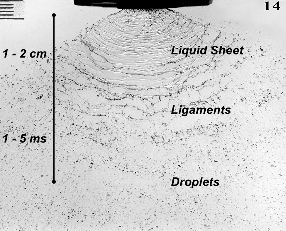
    Hydraulic atomizers comprise the majority of agricultural nozzles. They work by forcing a liquid through an orifice, resulting in a liquid sheet that is inherently unstable. The sheet breaks into ligaments and eventually droplets within a few centimetres of leaving the nozzle. The physico-chemical properties (elongational viscosity, dynamic surface tension, etc.) of the liquid affect the shape of the sheet and its stability, and therefore play a role in atomization.

    The dimensions of the liquid sheet depend on the nozzle type and the conditions in which they release the liquid. Flat fan nozzles, the most common in agriculture, force the liquid through an elliptical orifice that results in a sheet that is thicker in the middle and tapers at the edges. Nozzles that produce wider fan angles have narrower orifices, creating thinner sheets that ultimately produce finer sprays. Higher flow rate nozzles produce thicker sheets. A deflector nozzle impinges a stream of liquid against a plate that forces the stream flat and spreads it out, creating a different set of forces that destabilize the sheet. A cone nozzle generates a swirling action that results in a less stable sheet.

    Fig. 1: Three stages of hydraulic atomization of a flat fan nozzle. A sheet emerges from the exit orifice, which becomes unstable, forming ligaments that ultimately break into droplets (Image Source believed to be Silsoe Research Institute)

    If we place these nozzles into an airstream, either from travel speed or ambient wind, the spray sheet will become less stable and result in finer sprays. The amount of air-shear atomization will depend on the relative orientation of the nozzle sheet and the moving air. Nozzles that spray parallel to moving air produce less air shear and therefore result in coarser sprays than nozzles oriented perpendicular to the air stream. This characteristic is exploited by aircraft as a means of droplet size control, having a greater effect than spray pressure. 

    Rotary atomizers, either from rotary cages or spinning disks, are capable of producing sprays whose droplet size ranges are more uniform than those from traditional hydraulic atomizers. This produces advantages ranging from improved drift management to better use of available carrier volume. Rotary atomizers are popular with aerial applicators and are found on the majority of spray drones.

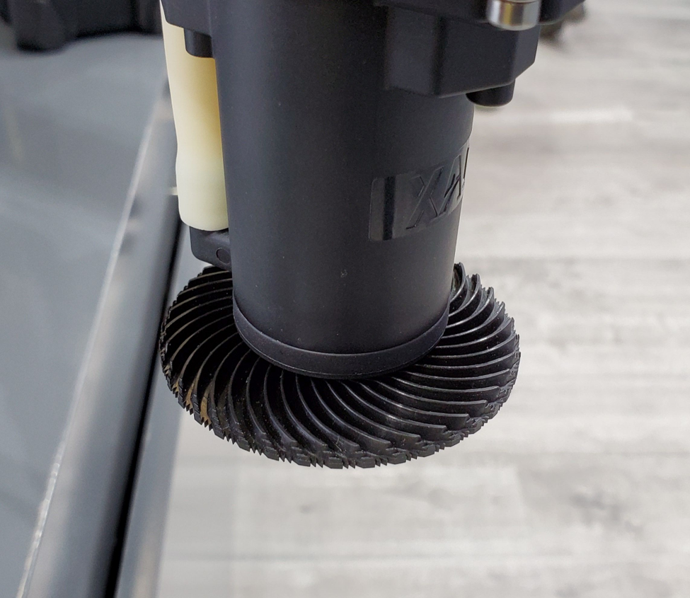
    Fig. 2: Rotary atomizer on a spray drone. Water is moved to the edge of a serrated disk by centrifugal force, forming ligaments that break into droplets

    Rotary atomizers create finer sprays when their rotational velocity is increased, or when the flow rate of the nozzle is decreased. In both cases, the ligaments formed at the periphery of the atomizer are thinner and will break up into smaller droplets. One disadvantage of rotary atomizers is the limited flow rate that they can atomize. For high flow rates, rotary cages, which break up the spray liquid by passing it through a series of wires mesh stages, are used. These require a fair amount of power, making them impractical for most smaller drone sprayers. 

    Droplet size ranges

    All hydraulic agricultural sprays are said to be polydisperse. This means that they are made up of a number of droplet sizes ranging from perhaps 5 µm to 1000 µm, or even 2000 µm or more for low-drift nozzles. How should the spray cloud be described?

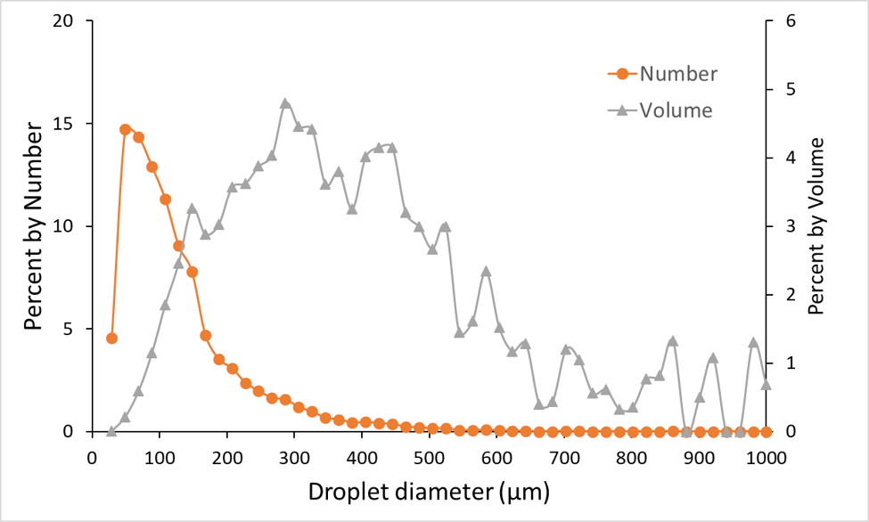
    The vast majority of droplets in hydraulic sprays are small. In any sample of flat fan nozzles, low drift or not, about 80 to 90% of the total number of droplets will be less than 150 µm in diameter. This held more or less true for a wide range of nozzles. As a result, using a traditional weighted average droplet diameter was not useful as a descriptor because the abundant sizes would always control the outcome even though they contained a minority of the spray volume. The contribution of the larger, but less abundant droplets would be hidden with an arithmetic mean.

    Any other descriptors based on droplet number alone, such as mode (the most frequent size class) or median (the size class above and below which were an equal number of droplets) are equally dominated by the high abundance of the smaller droplets.

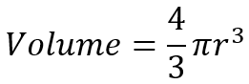
    To solve this problem, droplet diameters can be converted to their volume equivalent using the formula


    Where r is the radius of the droplet.

    This is relevant because the dose of pesticide in a droplet is related to its volume. It’s important to understand the contribution of relatively few larger droplets in terms of how this dose was received by plants.

    Fig. 3: Number and volume distributions of a typical agricultural spray (Wilger SR11005 @40 psi)

    Thus we arrive at a volumetric distribution, where each diameter is described by the proportion of the total spray volume it represents. That volume represents the dose of spray. Now we have some practical meaning of the numbers.

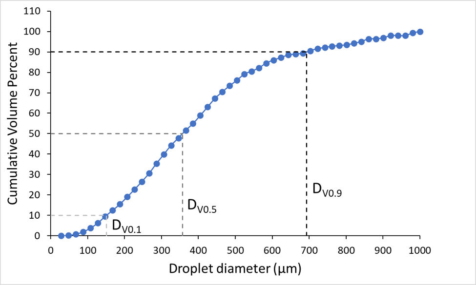
    First we generate a cumulative volume distribution. The volume contained in each size fraction is expressed as a percentage of the total volume and these are added together.

    The cumulative distribution can now be divided into benchmark values so we can get values that differentiate various sprays. The key ones of interest are the 10th, 50th, and 90th percentile. The 10th percentile, known as the DV0.1, is defined as the diameter below which is 10% of the total volume of the spray. DV0.5 and DV0.9 likewise describe the diameters below which are 50% or 90% of the spray volume, and the former is more commonly known as the Volume Median Diameter (VMD). Recall that the median is the value that divides a distribution in half by number, therefore the 50th percentile is also the median.

    Fig. 4: Cumulative volume distribution of Wilger SR11005 @ 40 psi. Dashed lines show DV0.1, DV0.5, and DV0.9.

    The VMD is the benchmark value, it can be thought of as the diameter near which the majority of the dose is delivered. The DV0.1 can serve as a drift index, describing the diameter that contains the smaller droplets. Sprays that are more drift-prone have lower DV0.1 values. The DV0.9 can be an index of the droplets that may not be able to contribute much to product efficacy because they are too big to cover much area, and they are likely to be very rare, possibly missing the target altogether. Higher DV0.9 values indicate that more of the spray may be lost to large droplets that will likely rebound.

    All of these parameters are related to each other. A finer spray will have lower DV0.1, DV0.5, and DV0.9 values. But it is not necessarily correct to say that a spray with a lower DV0.5 will have less drift potential. Some nozzles, by virtue of their design, can have smaller driftable size fractions as well as a lower DV0.5.

    One of the main reasons that sprays of equal DV0.5 may have different behaviours in the environment is their Span. Relative Span describes the uniformity of the droplet sizes in a spray. A perfectly uniform spray (containing droplets that are all the same size) will have a span of 0 because all three volumetric parameters will be equal.

    We sometimes encounter the Sauter mean of a spray, which can be defined as the diameter of a drop having the same volume/surface area ratio as the entire spray. This is useful when surface area is of importance, such as in combustion or evaporation.

    The popularity of laser measurement systems, and their ability to measure droplets that previously escaped detection, was a boon to the spray industry. But it quickly became clear that simply comparing these parameters was problematic. Each laser system, and indeed each laboratory that used them, seemed to create their own unique values for the same nozzles. We will explore the solution to this problem in Part 3.

  • What is Spray Quality, Part 1 – Measuring Droplet Size

    What is Spray Quality, Part 1 – Measuring Droplet Size

    It’s often been said that droplet size is the most important factor governing spray operation success. Both spray drift and pesticide efficacy depend to a large degree on droplet size. For something this important, the droplet size information from nozzles ought to be accessible and easy to understand. 

    There are a few problems to overcome before we get there.

    The first is the difficulty in measuring droplets in the first place. Spray droplets are very small and evaporate quickly.  In the early days of spray technology research, sprays would be captured on a surface and individual droplets measured and counted under a microscope. A common approach was to use magnesium-oxide coated glass slides. The magnesium oxide layer was soft, and an impinging droplet left a tell-tale crater behind, much like those found on the moon’s surface. This allowed the analysis to be done after evaporation. Magnesium oxide does a great job but relies on droplets having enough momentum to leave their mark. There is also a spread factor (ratio of crater diameter to droplet diameter) that has to be known.

    Water-sensitive paper (WSP) is the modern version of this concept, and we’ve written much about the topic. Jason in particular has done a deep dive on how WSP works and how it’s analyzed.

    We can also add dye to spray mixtures to see deposits on various glossy paper surfaces.  The resolution of the dye-droplets can be better than those from WSP but their deposits can also be so faint that they pose thresholding and analysis problems.

    The great thing about impingement methods like WSP is that they’re easy to use, and they are particularly useful for a quick visual and qualitative assessment of coverage. If wanted, coverage can be quantified by scanning the WSP for percent area covered or deposit density.

    Droplet size determination is problematic on WSP because one needs to know the spread factor (how much larger the deposit is compared to the in-flight droplet that caused it) to back-calculate the original size of the in-flight droplet.

    Spread factor depends on droplet size, velocity, formulation, and the nature and orientation of the surface it’s collected on. The SF formula provided by the paper manufacturers is a good start but it is far from perfect.

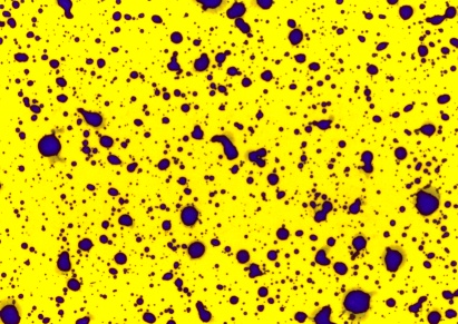
    Fig. 1: Water-sensitive paper (WSP) treated with a Very Coarse spray at about 100 L/ha. Note the coalescence and overlap of some deposits.

    In addition, the overall droplet density has to be low enough to avoid overlaps or coalescence. Usually a water volume over 50 to 100 L/ha will create issues. The WSP also has to collect the droplet in the first place. Smaller droplets often move around larger objects such as a leaf, or a similar sized piece of paper. If they impact at a sharp angle, the deposit will be elongated due to smearing and that creates additional difficulties.

    Even if the paper collected the smallest droplets, they may not appear as stains. Droplets below a certain diameter (about 50 µm) do not leave a visible deposit on the paper. 

    So, while WSP is a great tool for visualizing a deposit, its limitations usually prevent it from being used to accurately measure the droplet size spectrum of a spray. 

    The Rise of the Laser

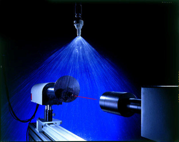
    In the 1970s and 80s, we saw the introduction of laser-based droplet size measurements. With these, a spray simply needed to be directed into a such an instrument, and it very quickly determined the diameter, and in some cases, the velocity, of the droplets. The principles employed by various laser instruments differed, and although one could now rapidly obtain data in-situ, the numbers among the instruments didn’t always agree.

    Fig 2: Laser instruments help to measure droplet size of sprays (photo source: TeeJet)

    The Most Common Laser Systems

    Laser diffraction: One of the first droplet sizing instruments is manufactured by Malvern (https://www.malvernpanalytical.com/en), and is still in use today. A laser beam passes through a spray cloud. The system uses a laser diffraction principle that works as follows, according to Malvern: “Large particles scatter light at small angles relative to the laser beam and small particles scatter light at large angles. The angular scattering intensity data is then analyzed to calculate the size of the particles responsible for creating the scattering pattern, using the Mie theory of light scattering.”

    To calculate the droplet sizes responsible for the scattering behaviour, the laser system has light-sensitive sensors in concentric circles behind the spray plume. When a sensor in the middle of these rings picked up a signal, it likely originated from a larger droplet because of its lower light scattering properties. Sensors further from the centre picked up smaller droplets. The system thus had an idea of the relative frequency of the various droplet sizes in the spray cloud and modelled these according to the classic Rossin-Rammler spray distribution model, from which descriptive parameters are calculated.

    Laser diffraction is the most popular method for in-situ droplet sizing. The company Sympatec (https://www.sympatec.com/en/) also offers a system that competes with Malvern that is found in many labs.

    Laser Shadowing: The Particle Measuring Systems (PMS) system was one of the earliest laser systems. It was a very compact and sturdy system that shone a laser light at the spray cloud and the droplets in that cloud cast shadows against a sensor array a fixed distance away. The size of these shadows could then be measured to arrive at a droplet size distribution. The PMS was particularly good at measuring small droplets.

    Although long discontinued, the PMS system had the basic appearance of a torpedo and was often mounted on aircraft or in wind tunnels to measure cloud aerosol sizes. Very cool. The company still manufactures other particle measuring devices (https://www.pmeasuring.com/).

    Pulsed Laser Illumination: This is a different approach to the laser shadowing of the PMS system. Oxford Lasers systems (https://oxfordlasers.com/) use a video camera to view the spray cloud and freeze images from using a very high frequency pulsed laser light. This light illuminates the cloud briefly which allows a still image to be briefly displayed.  Image analysis then measures the diameter of each particle in the image, adjusting for out-of-focus images.  It’s possible to analyze the speed and direction of the particles by comparing the particle position in subsequent images. This system is quite popular among scientists due to its ease of use. A portable unit that can be deployed in fields is available.

    Phase Doppler: In the mid 1980s, a system was developed that uses the Doppler principle to measure both the speed and diameter of droplets. Two out-of-phase laser beams intersected in a spray cloud, and a droplet passing through the intersection point created a Doppler burst that signalled the speed of the droplet. The burst signal also contained information on the droplet diameter, derived from a frequency shift of the two laser beams utilized in the system. This system has very high data acquisition and was the first to create a temporal sample of the spray, increasing the accuracy of the droplet size measurements.

    Initially brought to market by Aerometrics (later acquired by TSI) and called the Phase/Doppler Particle Analyzer (PDPA), it is now mainly offered by Dantech systems (https://www.dantecdynamics.com/).

    Sampling Bias: Temporal vs Spatial

    It’s not straightforward to measure a sample of moving objects. It may seem intuitive that if one wants to know how many objects are present, taking a picture and counting the objects would provide the answer. But when objects move at different speeds, that answer will be incorrect because the slower moving objects will be over-represented.

    Let’s assume you’re working on a traffic count project to understand the number of people crossing a bridge either walking or cycling. Let’s also assume that one walker and cyclist depart for the bridge every 5 seconds, i.e., there are the same number of each. If you wait until the bridge is full of people crossing and take a picture it will show more people walking on the bridge than riding bicycles. That is because the bicycles are faster and many will already have left the frame.  Thus counting the number of people in the picture over-estimates the number of walkers because they move slower.

    The same problem arises with these laser systems because in a hydraulic spray, the smaller droplets move slower than the larger droplets. Any system that takes a picture and counts what’s in it will have what’s called a spatial sample, overestimating the slower (smaller) droplets.

    A temporal sample can measure the velocity of the droplets and therefore account for their speed, giving a more accurate measure of the abundance of the droplets. In the case of the PDPA, it acheives this simply by counting all the individual droplets that pass, in sequence, through its meassurement area, called the probe volume. As they pass, it notes their velocity and diameter.

    To address this issue with a spatial sampling instrument, many labs now use wind tunnels and direct the spray to be tested with the wind direction. This forces the droplets to move at more or less the same velocity as the wind, eliminating or at least minimizing the speed differences before the droplets reach the laser instrument.

    WSP produces a temporal sample because it ultimately catches all droplets, but it has different types of sampling bias. Large deposits usually cover smaller ones. Smaller droplets may not impact on the target due to poor collection efficiency. Small droplets may dry too quickly to leave a visible stain. As a result, even if we had accurate spread factors, we would tend to under-estimate the number of smaller droplets, opposite of the error of spatial systems.

    Scanning the pattern

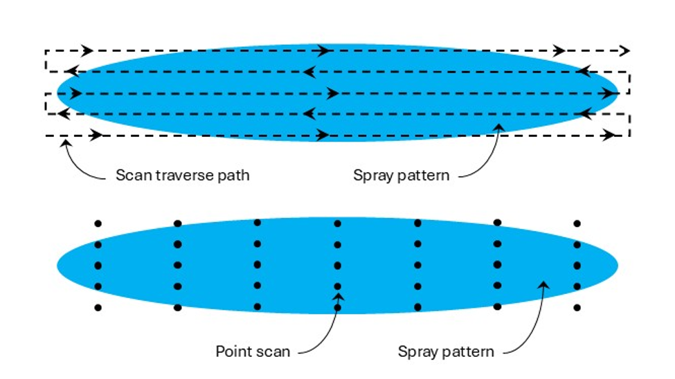
    Droplets are not distributed uniformly within a spray pattern. In a flat fan nozzle, for example, the centre of the pattern contains the smaller droplets. The outside edges of the pattern contain fewer small droplets and more large droplets. Some laser systems have a very shallow depth of field, and the PDPA is a point-measurement. As a result, it is not accurate to simply point the measuring device at a single location of the spray pattern. Accurate droplet size spectra from lasers requires a thorough traversing scan of the spray pattern along at least its long axis, and preferably two or more such traverses at increasing distances from this central axis. The scanning method would likely need to be adjusted to suit various types of atomizers, such as hollow cone nozzles.

    If no traversing mechanism is available, it is acceptable to measure the spray at several discrete locations and then merge the data prior to analysis. In all cases, three replicate samples should be taken so that an estimate of variability is available.

    Many labs, having compared a full scan with many traverses to those with fewer traverses have opted for a simple back and forth traverse with little loss in accuracy.

    Fig. 3: Possible ways of scanning a spray pattern for droplet size analysis. Top: traversing scan. Bottom: point scan

    Sometimes sprays are atomized within a chamber to prevent the droplets from contaminating the surrounding area if they contain any active ingredients. These chambers can also add measurement errors from, say, small droplets that recirculate within the chamber, or due to any glass surfaces through which the laser lights must pass. These all need to be considered, as they add to the many variables that create different results even when comparing identical sprays between labs.

    In Part 2 we discuss how to use the information we gather from droplet measurements. As you might expect, this is also not as straightforward as it seems.

  • Airblast Nozzles – Distributing Flow

    Airblast Nozzles – Distributing Flow

    There’s a certain deer-in-headlights expression that creeps onto a sprayer operator’s face when we discuss nozzle selection. We sympathize with our field sprayer clients given the variety of brands, styles, flow rates and spray qualities they must choose from. And PWM has made the process even more complex. However, airblast operators face an additional challenge; Unlike horizontal booms, vertical booms often distribute the flow unevenly to reflect relative differences in the distance-to-target and the density of the corresponding portion of target canopy. We discuss the broader, iterative process of nozzling an airblast boom here, but in this article we focus on the topic of flow distribution.

    An overwhelmed operator trying to nozzle a boom.

    The question of “which rate goes where” is still debated. It’s led to diagnostic devices called Vertical Patternators which show the profile of the spray. Operators can use these to visualize their distribution… but they are few and far between. For the rest of us, deciding on the best distribution begins with understanding how the practice evolved.

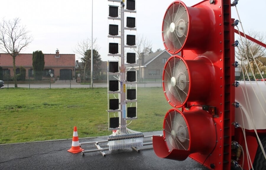
    The AAMS vertical patternator. The mast moves back and forth across the swath of a parked sprayer. Each black collector intercepts the spray at different heights. The fractions collect in the tubes at the bottom to show relative volume.
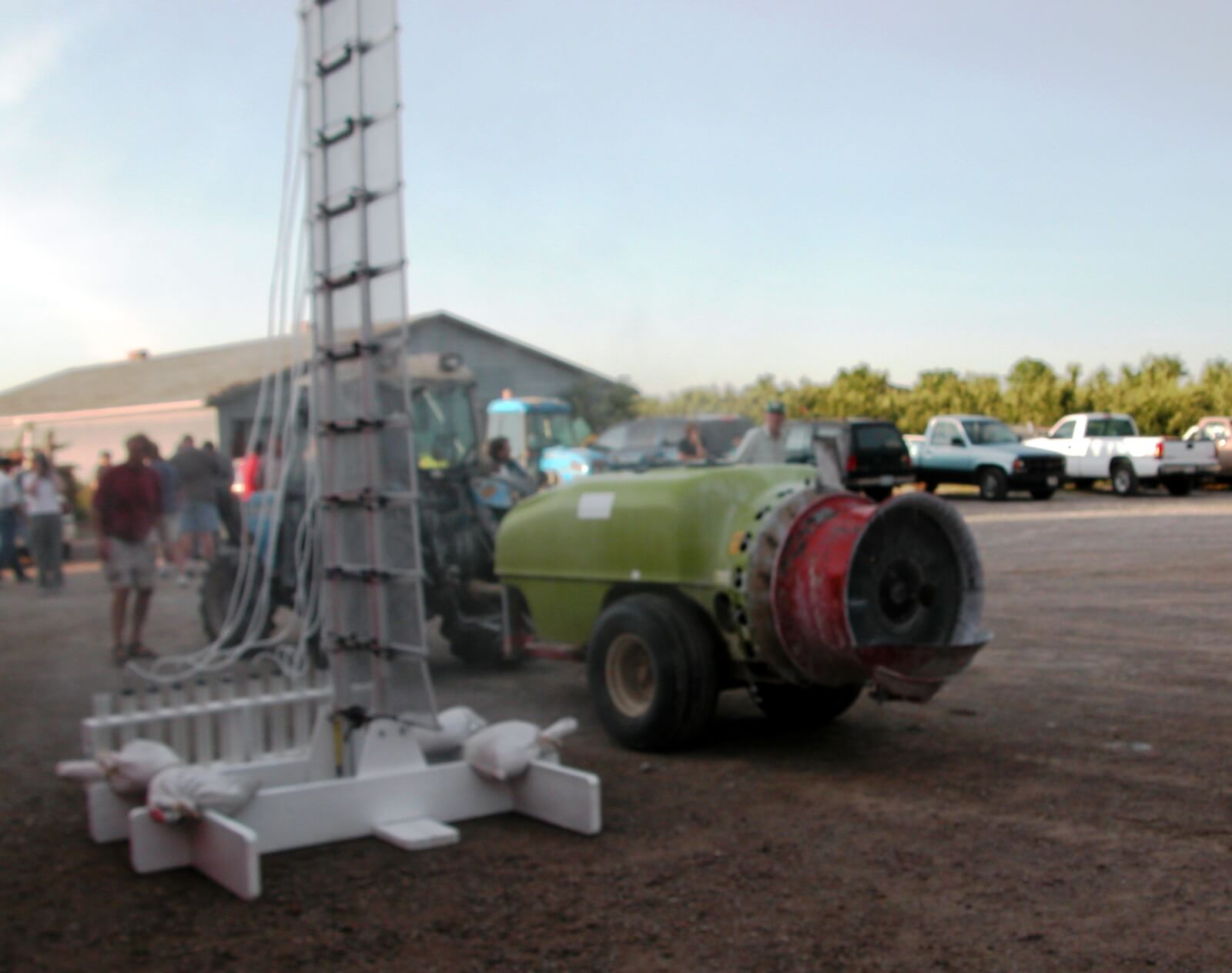
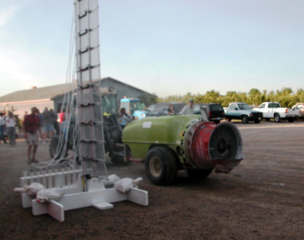
    A blurry shot of an OMAFA-built vertical patternator. The sprayer parks in front of the screens, which intercept spray. It’s collected in troughs and runs into columns that show relative volume.

    1950s

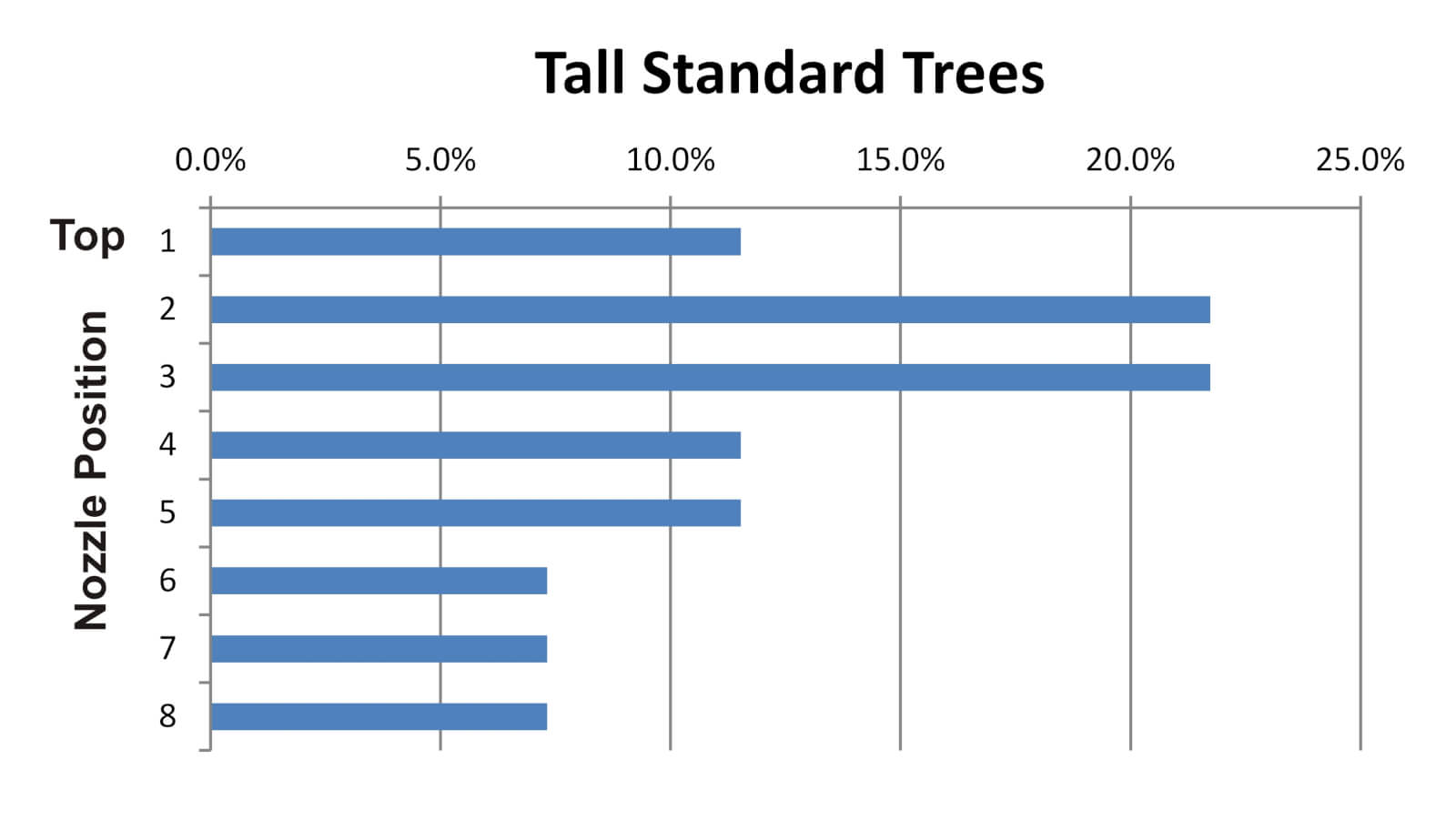
    In the 1950s, the mantra was to blow as much as you could, as hard as you could, and hope something stuck. At the time, John Bean promoted a method called “The 70% Rule” whereby operators used full-cone, high volume disc-core nozzles to emit the vast majority of the spray from the top boom positions. John Bean provided a slide-rule calculator to help operators configure booms to align the top nozzles with the deepest, densest portion of the 20-25 foot standard trees they were trying to protect. Back then, most airblast sprayers were engine-driven low-profile radial monsters capable of blowing to the tops of those trees. The practice persisted into the 60s and was encouraged by Cornell University (Brann, J.L. Jr. 1965. Factors affecting the thoroughness of spray application. N.Y. State. Arg. Exp. Sta. J. paper no. 1429).

    The profile of the spray would have looked something like the following graph:

    1970s

    In the 70s, extension specialists began advising operators to tailor the distribution to match the orchard spacing, tree architecture, canopy density and weather conditions. we reached deep into our archives for the Ontario Ministry of Agriculture and Food’s 1976 publication entitled “Orchard Sprayers” to see what we used to tell airblast operators.

    The 1976 update of Ontario’s 1971 “Orchard Sprayers” guide. A trove of hard-earned knowledge that still has relevance today. I love that the Minister’s name, and not the author’s, is on the cover. Let’s set the record straight: R. W. Fisher, D. R. Menzies and A. Hikichi, based in Vineland and Simcoe, Ontario.

    Here’s a synopsis of what was advised:

    1. Choose a tree size and shape that is typical of your orchard and park the sprayer at the normal spraying distance from it.
    2. Find one or two middle nozzle position(s) and air deflector or vane settings that direct the spray up through the top-inside of the tree. This is called the “middle volume zone”.
    3. Find rates that will give a large output in this middle volume zone, and smaller outputs for positions above and below.
    4. The total output must still add up to the target volume.

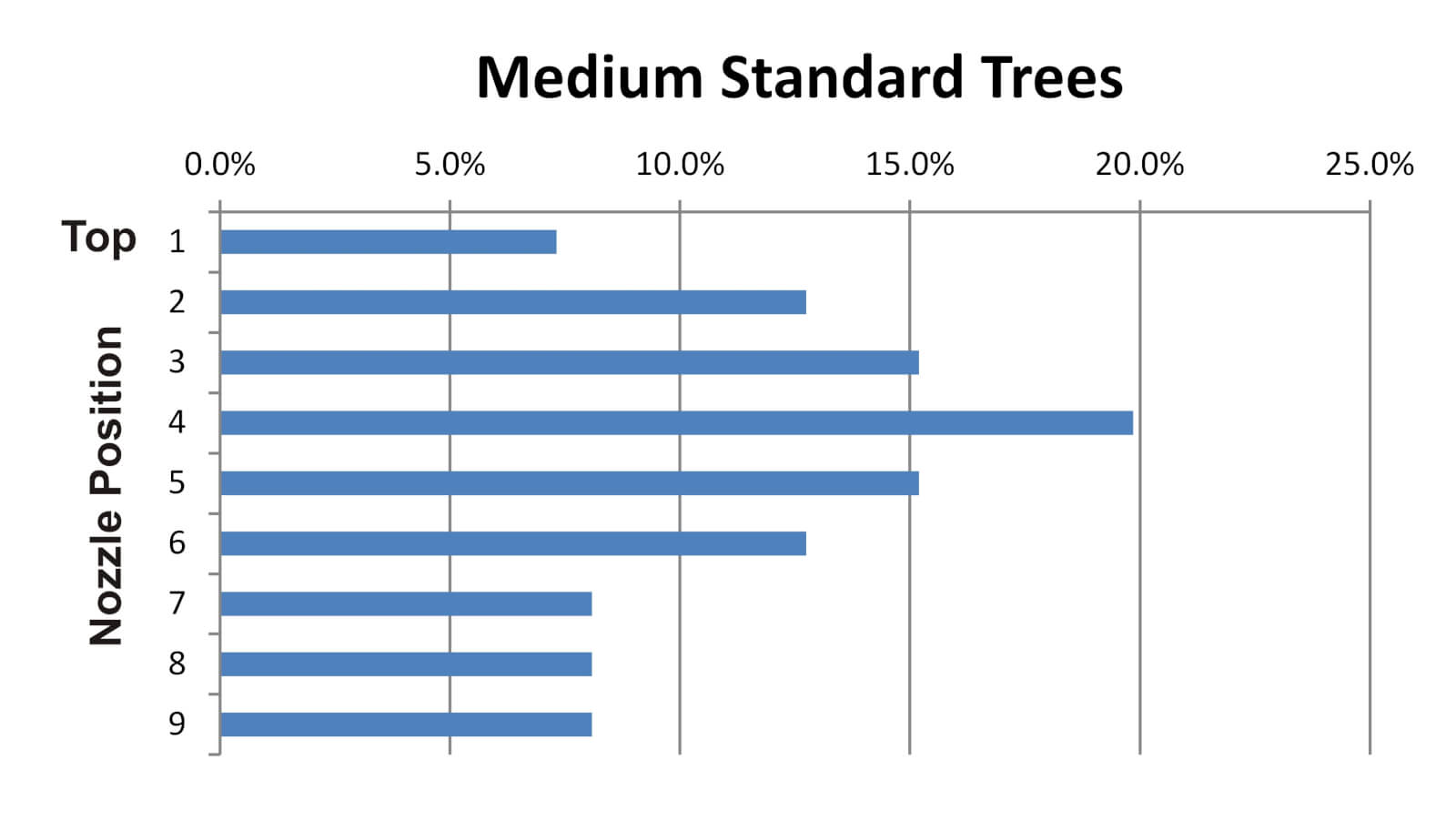
    It seemed operators were getting away from high rates in the top positions and instead shifting the distribution to match the canopy shape and density. If we were to follow these recommendations, the spray profile would look something like this:

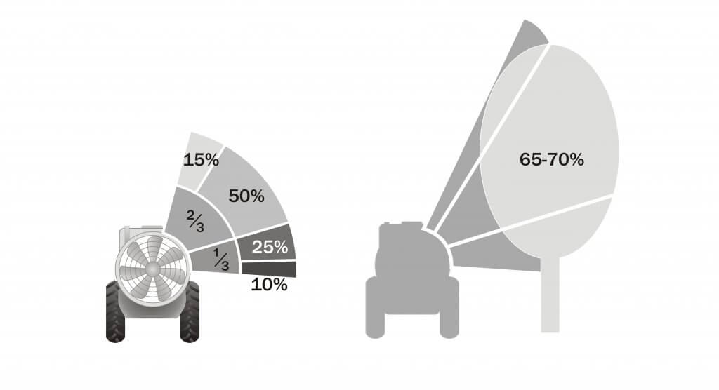
    Later, Agriculture Canada’s 1977 publication entitled “Air-Blast Orchard Sprayers – A Operation and Maintenance Manual” had similar advice. Here we find the “2/3 boom rule” as the authors state: “To ensure good distribution through the trees, about two-thirds of the spray should be emitted from the upper half of the manifold.”

    1980s

    Operators followed this approach well into the 80s, as they endeavored to aim the majority of the spray into the densest part of the canopy. Many can relate to the following illustration that divides the boom, which I modified from an array of period factsheets. The fractions represent the portion of the available boom. The percentages indicate the relative volume. Of course, it matters how large and how far away the target is for either the 2/3-boom or 70% rule to make sense (the middle volume zone is shown receiving 65-70% in the silhouette).

    1990s-2000s

    The 2/3 or 70% rules still work for standard nut and citrus trees, and perhaps for large cherry trees, but pome and tender fruit orchard architecture is densifying at this point in time. In the 90s and 00s we started transitioning from semi-dwarf into trellised, high density orchards.

    Leaping to 2005, Ohio’s Dr. Heping Zhu et al., found that a high density orchard is effectively sprayed by the same rate in each nozzle position. They wrote: “[Historical] recommendations are to use a larger nozzle at the top of each side, with the capacity of the top nozzle at least three times greater than other individual nozzles. However, results in this study with three different spray techniques showed that spray deposit was uniform across the tree canopy from top to bottom with the equal capacity nozzles on the air blast sprayer.”

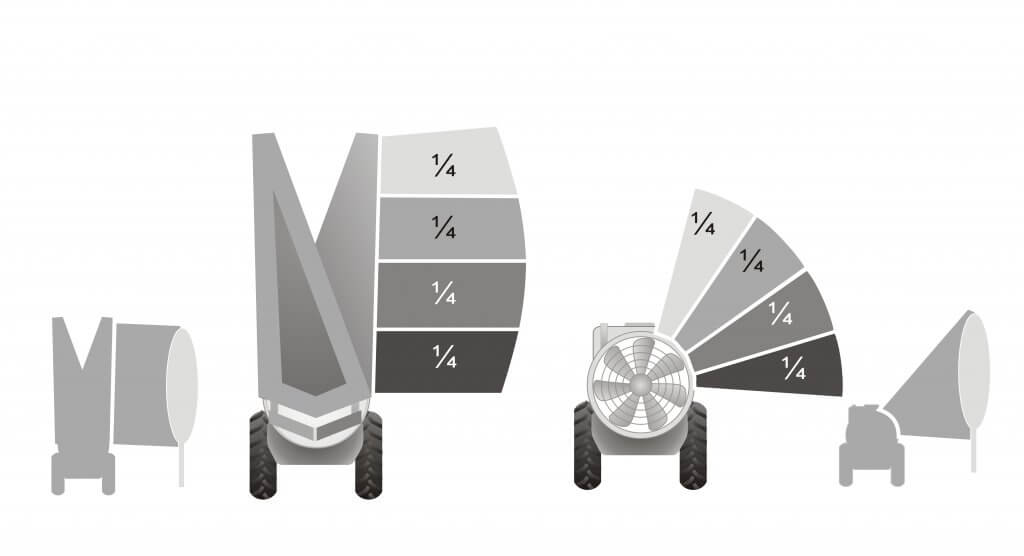
    What a pleasant surprise to simplify our lives! If we can use an even distribution for dense, nearby trees, it follows that any vertical crop with the same width and density located close to the sprayer (e.g. cane fruit, trellised vines, etc.) would benefit from even distribution:

    Today (2020s)

    So, how do we do it today? There is still no simple answer; Conditions change, not all sprayers are the same, and not all applications have the same target. Let’s build on what history has taught us and establish a process to achieve better coverage uniformity and reduce waste.

    No matter the crop, the operator must first adjust air settings. Air volume and direction play the most critical role in transporting a droplet to (and into) a target canopy. Too high an air speed will cause spray to blow through the target, rather than allowing it to deposit within. Aim the air just over, and just under, the average canopy. Ensure there’s enough air to overcome ambient wind and to push the spray just past the middle of the target canopy.

    It should be noted that we assume the operator is spraying every row. With certain exceptions, alternate row middle spraying is not generally recommended. Not only can it compromise coverage on the far side of the target, it makes it far harder to match the nozzling on a single-row sprayer and is a sure-fire way to increase drift.

    Next, determine which nozzles are not needed (e.g. spraying the ground or excessively higher than the top of the canopy). Remember: hollow cones overlap very close to the boom and spread as much as 80°. Airblast sprayers rarely if ever need the lowest positions and unless spraying overhead trellises they may not need the highest either. Turning off the highest, and most drift-prone, nozzle positions in high density orchards is illustrated in the logo I was asked to create for Washington’s short-lived Pound the Plume awareness campaign in 2017.

    Then, finally, we decide on distribution. If the crop is nearby and relatively narrow, you can try even distribution. If you elect to distribute the spray unevenly to better match the variable-width target, or compensate for distance, aim half the overall output at the densest part of the canopy (the middle volume zone). Consider how the following factors might influence your choices:

    1. High humidity means more spray will reach the target, and vice versa. This is because all droplets are prone to evaporation. We have heard it said in hot, dry conditions (described by Delta T), a droplet can lose ½ its diameter every 10 feet. As they evaporate they get lighter, meaning they are less subject to their original vector and the pull of gravity, and more subject to deflection by wind. The use or coarser droplets, and/or humectants, can help, but higher volumes can help too – they increase the odds of some droplets hitting the target and actually humidify the air to slow evaporation.
    2. Windspeed increases with elevation, so spray is most likely to deflect at the top of canopies where they have already lost size (and momentum and direction). Early in the season when there is little if any foliage, wind speeds are higher overall. This is why we advise adjusting air settings using a ribbon test before considering boom distribution – you need enough air volume, aimed correctly, to get the spray to the top.
    3. The denser and deeper a canopy, the more spray is filtered and unavailable for coverage. This is why you will always achieve more coverage on the adjacent, outer portion of a canopy versus the interior. In semi dwarf apple orchards we have seen the coverage drop by half for every meter of canopy. Finer spray can penetrate more deeply because there are more droplets and they move erratically, whereas coarser droplets move in straight lines and impact on the first thing they encounter. Higher volumes will improve penetration and overall coverage, but there is a diminishing return and runoff will occur more quickly leading to more waste.
    4. Further to the last point, remember that it’s the air that propels the spray, not the pressure. Higher liquid pressure can propel coarser droplets further, but has little effect on finer droplets. imagine throwing a golf ball and a ping pong ball into a light headwind and envision how they fly. Plus, the higher the pressure, the finer the mean droplet diameter.

    Confirm Your Work

    To know how all these factors play out, you must use water sensitive paper (or some other form of coverage indicator) to diagnose the results. Remember, the goal is uniform coverage and for most foliar products, we want to achieve a minimum coverage threshold of 10-15% and a droplet density of 85 deposits per cm2 on at least 80% of the targets.

    Taking the time to match your output to the target has the potential to greatly improve coverage and reduce waste. Nozzle body flips and quick-change nozzle caps make the process of switching nozzles between blocks fast and easy. It’s worth it.

    Grateful thanks to Mark Ledebuhr, Gail Amos and Heping Zhu who edited, corrected and contributed to this article.