Author: Jason Deveau

  • Spraying Ginseng with Arag Microjets

    Spraying Ginseng with Arag Microjets

    In June 2013 we ran a ginseng spraying workshop and we learned as much as the growers did. Ginseng is notoriously difficult to spray:

    • It is highly susceptible to pathogens given the high humidity and still conditions generally found under the shade structure.
    • It forms a solid ceiling of leaves that resist spray penetrating to the stem and crown below and makes under-leaf coverage very difficult to achieve.

    Many growers have (wisely) walked away from the old Casotti sprayers, which have been shown to give erratic coverage at best. They have adopted the Arag Microjet system with it’s characteristic orange shields. The >$80.00 CAD price tag for each nozzle is due to the brass mixing valve and swivel joint, as well as import costs from Italy. Contrary to popular belief, it does not use air-assist, or air-induction – it is strictly hydraulic. It does tend to create a ‘wake’ of air movement at high pressure. This phenomenon is called air entrainment and it is caused by large droplets travelling at high speed.

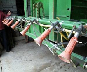
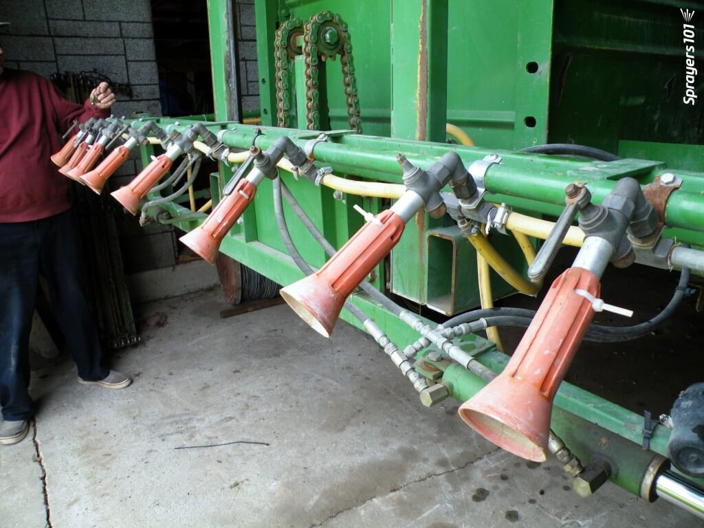
    Classic Arag microjet nozzles.
    Classic Arag microjet nozzles.

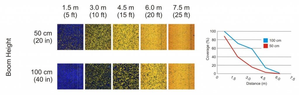
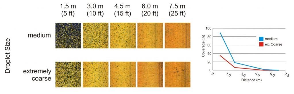
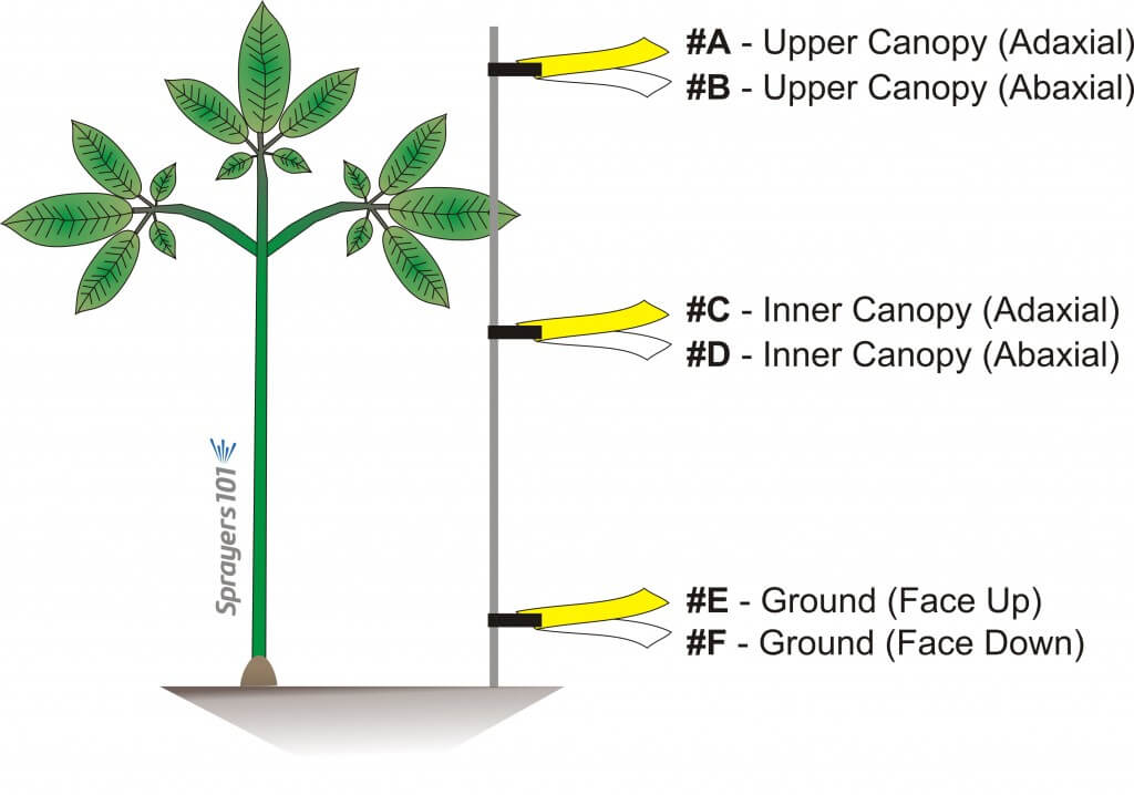
    This nozzle is essentially the business-end of a spray gun. The way it is used in ginseng it works more-or-less like a hollow cone disc-core assembly. This begs the question “Why not use the cheaper and more readily available ceramic disc-core?” We set out to compare the two options using water sensitive paper set within the canopy. These yellow, paper targets turn blue when sprayed, clearly showing spray coverage.

    Location of water-sensitive papers in the ginseng canopy.
    Location of water sensitive papers in the ginseng canopy.

    Determining rates

    The first step was to determine the output rate for each nozzle. Generally, nozzle manufacturers provide rate tables showing how much volume a nozzle emits by time (e.g. US gallons per minute) at a given pressure. Finding these tables for the 1.5 millimetre Arag Microjet proved difficult. When we finally found one, it was discovered the rates were established for 200 to 850 pounds per square inch. This is excessively high pressure for a typical boom sprayer, so tables had to be developed for lower pressures.

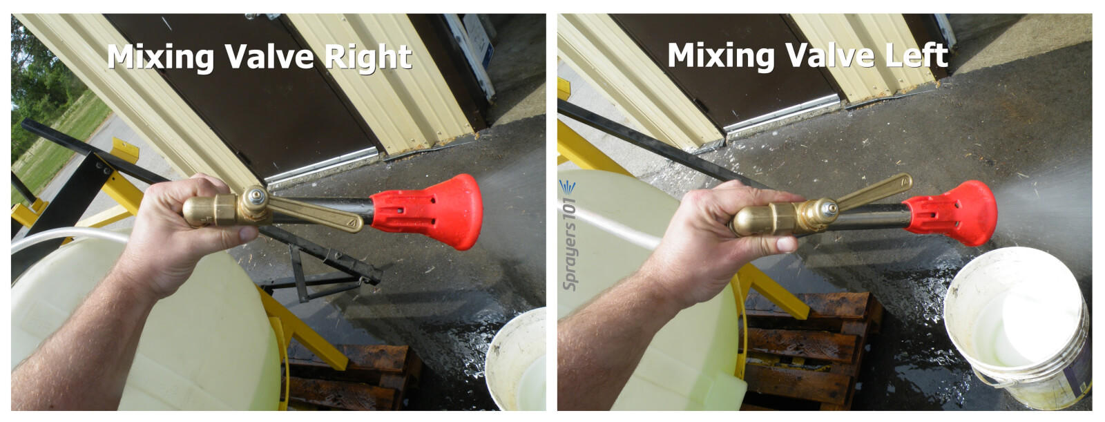
    Classic Arag microjets have a mixing valve that opens the spray up into a hollow cone, or collapses it into a tight stream. This also changes the rate. It can never be shut off completely, and it's hard to adjust consistently.
    Classic Arag microjets have a mixing valve that opens the spray up into a hollow cone (valve handle left or right), or collapses it into a tight stream (valve handle middle). The valve position also changes the rate. It can never be shut off completely, and it’s hard to adjust consistently.
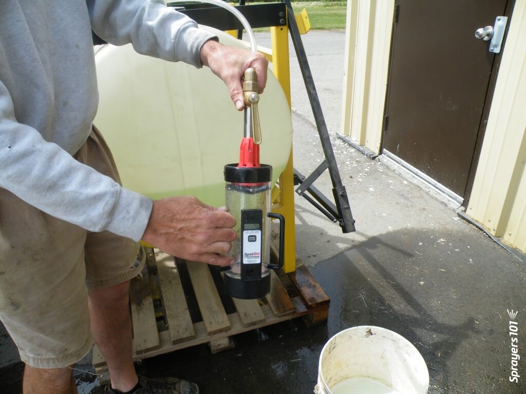
    Determining nozzle rate using the Innoquest Spot-On SC-4.
    Determining nozzle rate using the Innoquest Spot-On SC-4.

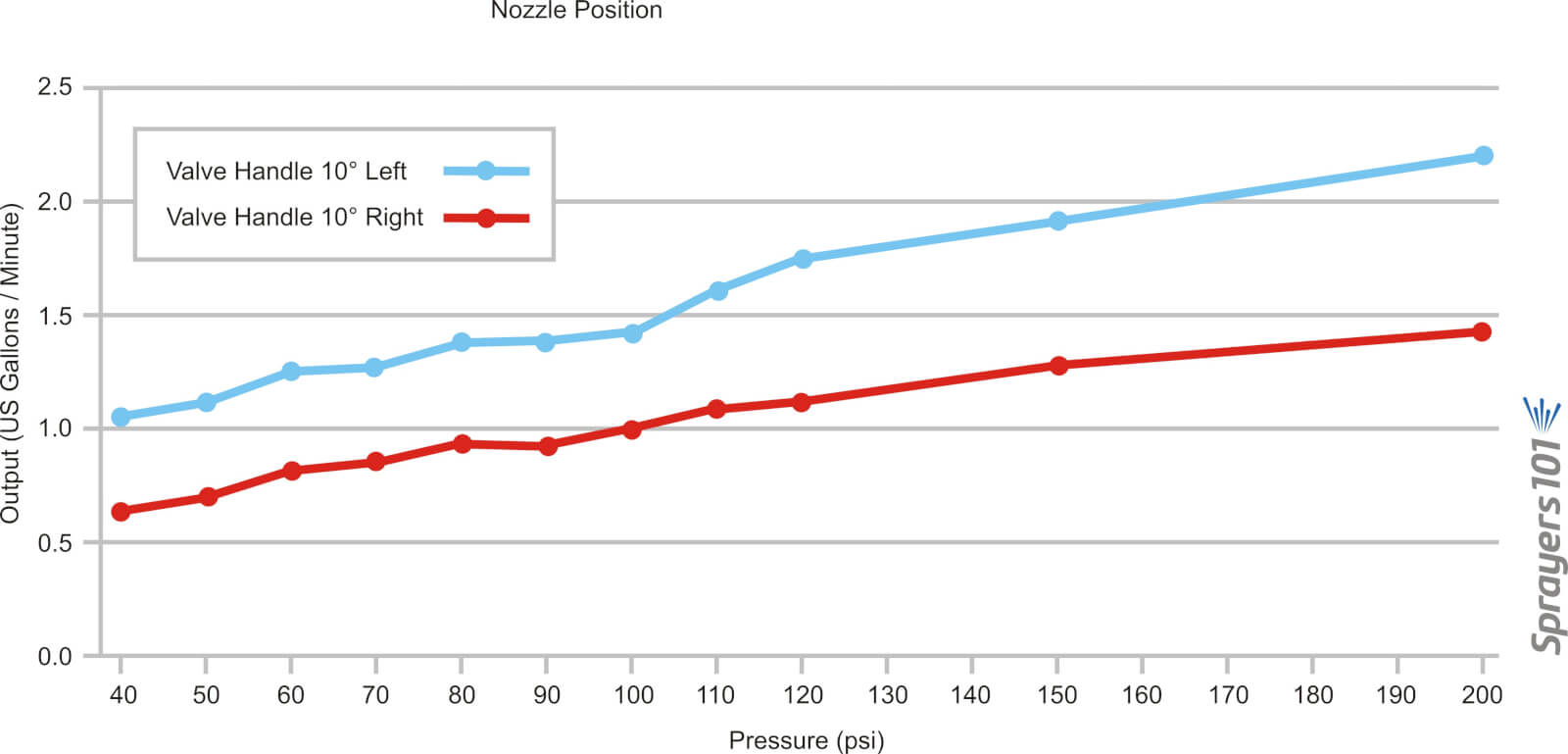
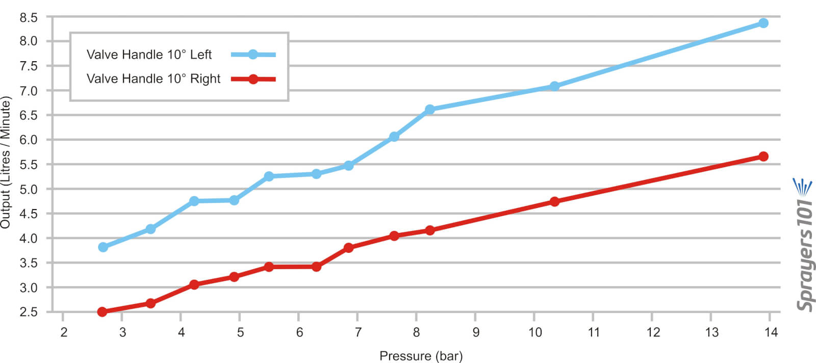
    Further, given the odd design of the mixing valve, it was determined that moving the handle ~10 degrees left of centre, or ~10 degrees right of centre, gave a difference of as much as 60%. The table below  shows the outputs for a 1.5 millimetre nozzle with the handle in both positions and the two graphs show the results… well… graphically. Outputs were determined using the Innoquest Spot-On SC-4, but the frothing effect created by the nozzles may have created minor errors. Each rate is the average of a minimum of three samples.

    Valve SettingPressure (psi)Avg Output (gpm)Pressure (bar)Avg Output (L/min)
    10 degrees left401.022.763.86
    10 degrees left501.13.454.16
    10 degrees left601.254.144.73
    10 degrees left701.254.834.73
    10 degrees left801.385.525.22
    10 degrees left901.46.215.3
    10 degrees left1001.456.895.49
    10 degrees left1101.67.586.06
    10 degrees left1201.758.276.62
    10 degrees left1501.8710.347.08
    10 degrees left2002.213.798.33
    10 degrees right400.652.762.46
    10 degrees right500.73.452.65
    10 degrees right600.84.143.03
    10 degrees right700.854.833.22
    10 degrees right800.95.523.41
    10 degrees right900.96.213.41
    10 degrees right10016.893.79
    10 degrees right1101.077.584.05
    10 degrees right1201.18.274.16
    10 degrees right1501.2510.344.73
    10 degrees right2001.3713.795.19
    Average 1.5 mm ARAG Microjet output at a range of pressures and two valve settings in US Imperial units.
    Average 1.5 mm ARAG Microjet output at a range of pressures and two valve settings in US Imperial units.
    Average 1.5 mm ARAG Microjet output at a range of pressures and two valve settings in Metric units.
    Average 1.5 mm ARAG Microjet output at a range of pressures and two valve settings in Metric units.

    Comparing nozzles

    Using the grower’s typical ground speed of 5 km/h (~3 mph) and operating pressure of 6.9 bar (100 psi), we found four TeeJet disc-core combinations that emitted a hollow cone pattern and approximately the same output as the Arag Microjets. The five nozzles sets tested were:

    1. ARAG Microjet® 1.5 mm = ~0.95 US g/min avg at 100 psi
    2. TeeJet® D8-DC25= 0.97 US g/min at 100 psi= ~97° cone
    3. TeeJet®D7-DC45= 0.97 US g/min at 100 psi= ~81° cone
    4. TeeJet®D4-DC46= 0.88 US g/min at 100 psi= ~33° cone
    5. TeeJet®D6-DC45= 0.93 US g/min at 100 psi= ~81° cone

    We did not use nozzle drop hoses (aka drop arms or hose drops) because it has already been firmly established that they are absolutely required to achieve under leaf coverage See OMAFRA factsheet 10-079 and this article.

    Observations

    While there were some complications with setting up the papers for the demo, we observed the following:

    1. The output of each Microjet nozzle can be as much as 50% more or less than expected without being visually detectable and output for each nozzle must be confirmed before spraying. Therefore, outputs should be confirmed before every application.
    2. Microjets at 100 psi emitting ~890 L/ha (~95 US gallons per acre) gave satisfactory coverage on all upward facing targets, but unsatisfactory under-leaf coverage. This has been demonstrated many times before.
    3. The TeeJet D7-DC45 combination emitting a similar rate gave satisfactory coverage on all upward facing targets, but unsatisfactory under-leaf coverage. They may be a viable alternative to the Microjets.
    4. Nozzle drops are advised to achieve under-leaf coverage.

    The demo also raised some questions:

    1. Did the TeeJet disc-core push the canopy apart as much as the Microjet? The audience noticed there was some leaf-shadowing where the cards did not get complete coverage using disc-core. This might have been coincidence, or it may not have. This question will be addressed in a research trial next season, but for now, the D7-DC45 appeared to give similar coverage to the Microjet.
    2. Can nozzle drops be avoided if pressure is raised to 27.5 bar (400 psi)? Thanks to one grower trying this experiment in his garden after the demo, we saw some under-leaf coverage is possible at such high pressures, but this occurred at the cost of a lot of noise, diesel fuel and considerable wear on the ceramic Microjet discs. The grower tested these tips and discovered they needed replacement after only two years of use. Nozzle drops are cheaper, easier and result in considerably more spray in the under leaf positions.
    3. We saw what minimal and excessive foliar coverage looked like, and determined how much variability there was from one nozzle to another. A significant question was “How much spray can be saved when using a more accurate application?” and the answer is yet to be determined, but could be well in excess of 10% of the typical spray volume. Given that this crop can be sprayed more than 100 times over it’s 3 or four years before harvest, this represents significant savings in pesticides and refill time.

    Additional – Newer ARAG Microjet Design

    Since this work was performed, growers have been exploring a newer option from ARAG.

    They are an improvement over the older version insofar as they are more easily calibrated and held at a given rate thanks to a lock nut. They still employ a 1.5 mm diameter ceramic disc, but this can be changed for a 1.0 or 1.2 quite easily. They are still somewhat finicky when trying to set a consistent spray quality and rate from nozzle to nozzle, but are better than the mixing-valve option.

    Learn more in this article.

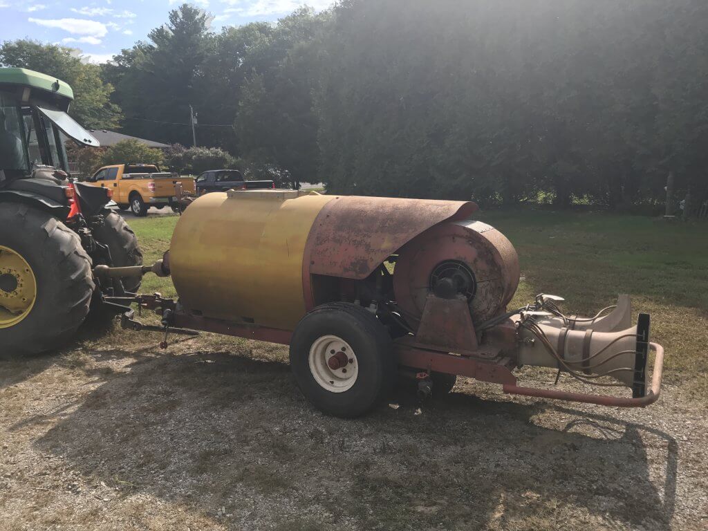
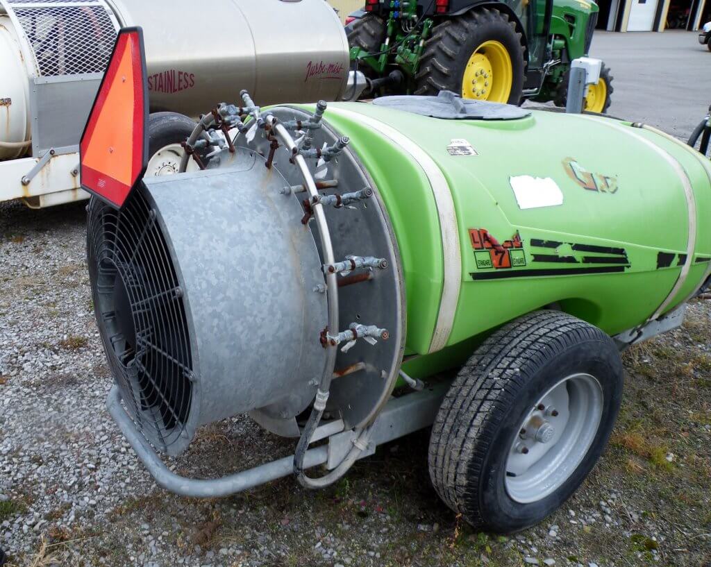
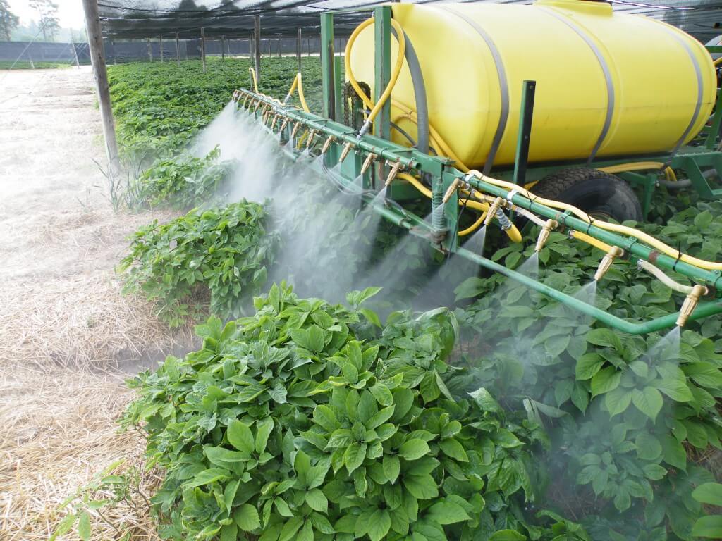
    Custom-made ginseng sprayer. A standard design.
    Custom-made ginseng sprayer. A standard design with newer, cheaper and easier-to-use ARAG microjets.

    Special thanks to Syngenta Canada for providing lunch, to C&R Atkinson Farms Ltd. for hosting, to TeeJet for supplying the disc-cores and water-sensitive papers, and to Dr. Sean Westerveld, Dr. Melanie Filotas and OMAFRA summer student Megan Leedham for contributing to the workshop.

  • Assessing Water Sensitive Paper – Part 3

    Assessing Water Sensitive Paper – Part 3

    This is the final part of our three-part article discussing methods for digitizing and processing water sensitive paper. You can read part one here and part two here.

    Morphological operations

    We can now move on to the larger shapes, or “morphology” of the objects in our binary image. Our goal is to quantify deposits by interpreting these shapes. Once again, these operations are powerful processing tools, but we must acknowledge three overriding limitations:

    1. Inconsistent stains

    Sometimes deposits do not create a consistent blue colour – they can get lighter or take on a greenish-yellow hue towards the perimeter of the stain. During thresholding, the outer edge can be accidently eroded, leaving behind an object with a jagged edge. This may lead us to underestimate the percent area actually covered. In the case of tiny stains, it might eliminate them entirely and lead us to underestimate deposit density.

    2. Overlaps

    It can be difficult to determine if an object represents a stain from a single droplet or is the result of multiple, overlapping deposits. This becomes significant when the surface of the WSP exceeds ~20% total coverage. The resulting objects may or may not have hollow centres where droplets do not overlap entirely. Misidentifying overlaps leads us to falsely conclude that an object is the result of a single, coarser droplet rather than multiple finer droplets.

    3. Ellipses

    Non-circular stains are formed when droplets scuff along the surface. Two droplets with the same volume encountering a paper at different angles can create stains with significantly different areas. We may wrongly conclude that the droplets that created them were coarser than they truly were. One approach is to use Feret’s Diameter (aka Caliper Diameter) by measuring the widest spans on the X and Y axes and taking the average. Another approach is to interpret the ellipse as a series of circular stains. Or we can decide to only acknowledge these objects when calculating percent area covered, but omit them when calculating deposit density or predicting original droplet size. Each strategy is a compromise, so it is important to be consistent and transparent when reporting results.

    Three common problems when analysing water sensitive paper.

    We’ll explore two morphological operations that can help us separate fact from fiction: Granulometry and Dilation-and-Erosion. We’re introducing these operations as part of the processing and detection step, but they may also overlap with the measurement step in our three-step process.

    Granulometry

    We can estimate the range of object sizes and get a sense of how they are distributed on the paper by filtering or “sieving” the image. Imagine pouring a mixture of sand and rocks through a series of ever-finer sieves. Doing so allows you to separate particles based on size exclusion. A granulometry function compares each object to a series of standardized objects with decreasing diameters. This isolates objects of a similar size and bins them in that size range. This is a powerful operation, but accuracy is lost when stains overlap to form larger objects. In this case, we move on to Dilation and Erosion.

    Dilation and Erosion

    Think of dilation as adding pixels to the boundary of an object. This makes tiny objects bigger, fills in any interior holes and can cause objects to merge. The number of pixel-wide dilations required to make objects contact one another can be used as a measure of deposit density.

    Erosion removes pixels from the outer (and sometimes inner) boundaries of an object. This eliminates tiny artifacts that may not actually represent stains. It can also split non-circular objects into multiple parts before shrinking them into multiple nuclei (aka centroids). These last-remaining points are not necessarily the centre of a stain, but the pixels furthest away from the original boundary.

    When a non-circular shape has more than one nucleus, they likely represent individual droplets that combined to form the larger stain. We can then use these nuclei to measure deposit density, such as in a Voronoi partition which triangulates each nucleus in relation to the two closest neighbours.

    Many image processers use both these operations sequentially. When an image is eroded and then dilated (a process called “Opening”), smaller objects are removed, leaving the area and shape of remaining objects relatively intact. Dilating and then eroding (a process called “Closing”) fills in small holes and merges smaller objects, once again leaving the area and shape of remaining objects relatively intact. We can use both of these functions to help smooth an image prior to measurement.

    (Top) Opening operations erode and then dilate the image. Moving left to right, the smaller objects tend to disappear. (Bottom) Closing operations dilate and then erode the image. Moving left to right, smaller objects either disappear or merge and holes are filled in

    Distance Transformations

    Distance transformations are advanced operations specifically used to separate objects that are densely packed. While not typically used when analyzing WSP, distance transformations are another means of identifying object nuclei. They are another means for teasing apart objects that are likely the result of overlapping deposits and then mapping their relative sizes and positions.

    Measurement

    The calculation of the area covered by deposits is straightforward. The pixels belonging to objects (the deposits) and those belonging to background are summed and then the fraction is converted to percent area covered. Research has shown that the image resolution does not significantly impact percent coverage assessments and has suggested that all image analysis software tends to produce similar results (+/- 3.5% observed when the same threshold was applied to multiple papers). This is acceptable because it’s within the variability inherent to spraying.

    We ran a similar experiment wherein we analyzed the same piece of WSP using four methods. Here are a few facts about the software we used:

    • DropScope produces images between 2,100 and 2,300 DPI. Currently, it ignores ellipses and doesn’t count anything spanning less than ~35 µm (3 pixels).
    • We set ImageJ to ignore any object spanning less than 3 pixels, which at 2,400 DPI was 30 µm in diameter.
    • Snapcard was a free app created by Australia’s GRDC. It was benchmarked using ImageJ, tended to underestimate coverage and was fairly inconsistent. Nevertheless, it was convenient for field work. Instances may still exist, but as of 2025 it no longer available through the GRDC.

    The images shown in the figure below were cropped from screenshots produced by each method. The actual ROI analyzed was ~3 cm2 for SnapCard, 3.68 cm2 for DropScope and 2.0 cm2 for both Epson/ImageJ methods. Our results indicate an +/- 4% difference in percent area coverage. This variability reflects the results of a 2016 journal article that compared SnapCard with ImageJ and other leading analytical software. That study claimed no statistically significant difference in percent coverage detected (standard deviations were about 20%). However, the ImageJ results tended to trend several percent higher than SnapCard. We saw this as well. And so, while resolution may not have a significant impact on percent area covered, there does appear to be some correlation.

    Percent area covered as reported by three image analysis systems. Only a minor difference was observed when resolution was doubled using the Epson/ImageJ method.

    Resolution definitely affects deposit counts. Particularly in applications that employ finer droplets. Consider the difference between detecting or missing 1,000 30 µm diameter objects. It may only amount to a fraction of a percentage of the surface covered, but +/- 1,000 objects on a 2 cm2 area is significant in terms of deposit density.

    Output

    Once a WSP image (or set of images) has been scanned, pre-processed, processed and measured, we will receive some manner of output. Some software packages create an attractive report with images, graphs and key values. These reports include percent coverage and many provide droplet density. Deposits may be binned by size, or spread factors are used to calculate the original droplet diameters and even estimate the volume applied by area. Other software packages provide raw data that can be imported into a statistical program or spreadsheet program like Excel for further analysis. Some software packages provide both.

    How far can we take this?

    Blow-by-blow data analysis is beyond the scope of this document, but how much weight should we give to coverage data obtained using WSP? The answer depends on the metric in question, but in all cases we must first acknowledge the three overriding caveats. Take it as said that they apply to everything that follows:

    1. Different brands (and even different production runs) of WSP can produce significantly different coverage metrics. When conducting experiments, use a single brand of WSP. Better still, use papers from the same production batch whenever possible.
    2. The same of piece of sprayed WSP can produce significantly different results depending on the software and protocol used to analyze it. When conducting experiments, use the same software and assessment protocol and be transparent about the process when communicating results.
    3. WSP coverage may not reflect the coverage achieved on an actual plant tissue surface. It is suitable as a relative index (I.e. papers can be compared to papers, but not to tissues) but the spread factor changes with surface wettability and the surface tension of the liquid sprayed. Note the differences in percent area covered in the following experiment with an organosilicone super-spreader:
    Difference in deposit spread on water sensitive paper versus a leaf surface using an organosilicone super-spreader and UV dye. The same volume was applied in each case and while the area increased two-fold on WSP it increased ~10-fold on an actual leaf. Image reproduced from work by Robyn Gaskin, Plant Protection Products, New Zealand.

    Recall that we started this document by listing the four pieces of information commonly sought using WSP. They were listed in order of reliability, and now we can explain why.

    • The percent surface area covered: We have established that this is the most reliable piece of data. Droplets do not spread on WSP the way they do on plant surfaces, so it will underestimate actual coverage. The results vary by analytical method, but it’s likely not dependent on resolution and still falls within the variability inherent to spraying. This metric gives us valuable and actionable information. We can say whether or not we hit a target, and evaluate whether a sprayer change resulted in more or less deposit.
    • The density of deposits on the target area: We have established that that there are limits to the reliability of this metric. It is affected by the analytical method used and can be greatly underestimated when resolution is poor or when deposits overlap in high numbers. Also, it will never reliably reflect deposits under 30 µm. Nevertheless, under controlled conditions this information does have value and is of great interest in enquiries about drift and contact fungicides.
    • The size of the droplets that left the stains: This metric is highly questionable except under controlled conditions. The many assumptions about surface tension, droplet speed, and droplet evaporation make it impossible to make definitive statements about spray quality. Finer droplets are greatly underestimated in this equation. Therefore, while there may be some value in using WSP as a relative index, this metric is a crude indication at best.
    • The dose applied to the target surface: This metric has not been discussed up to this point, but is quickly and easily dismissed. Let’s assume that a droplet with a high concentration of an active ingredient will leave a stain that is the same area as another droplet with a lower concentration. This will lead some to suggest that as long as the original concentration is known, we can back-calculate the dose (which is the amount of active on a given area). However, one droplet has the same volume as eight droplets that are half it’s diameter. This cubic relationship means that if they all deposit, the larger droplet will cover roughly 1/2 the surface area as the eight smaller droplets. Therefore, the smaller droplets spread the same amount of active over a greater area. Spread factor muddies this a bit, but ultimately it means that dose cannot be estimated from area covered. Dose is better assessed using collectors that permit the residue to be removed, such as Petri dishes, Mylar sheets, pipe cleaners, alpha cellulose cards, or glass slides.

    And so, the image analysis process described here is powerful and effective when used with water sensitive paper as long as the limitations are acknowledged. The same process can also be used with dyes and specialized collectors such as Kromekote to permit even greater resolution. But that’s another story.

    2026

    A new Brazilian cellphone-based system (SprayDex) emerged in 2026 that offers possibilities. Preliminary testing alongside other methods indicate it is consistent within itself, but as we saw in previous testing, the same WSP scanned using different systems will create different results. This is why, ultimately, WSP is a relative index and should only be compared within a given system; coverage cannot be reliably compared across WSP brands, or between digitization methods.

    2026 Comparison of three digitization / analysis methods. Same WSP was scanned each time.

    References (Further reading)

    Bankhead, P. 2014. Analyzing fluorescence microscopy images with ImageJ.

    Cunha, J.P.A.R., Farnese, A.C., Olivet, J.J. 2013. Computer programs for analysis of droplets sprayed on water sensitive papers. Planta Daninha, Viçosa-MG. 31(3): 715-720.

    Ferguson, J.C., Chechetto, R.G., O’Donnell, C.C., Fritz, B.K., Hoffmann, W.C., Coleman, C.E., Chauhan, B.S., Adkins, S.W. Kruger, G.R., Hewitt, A.J. 2016. Assessing a novel smartphone application – SnapCard, compared to five imaging systems to quantify droplet deposition on artificial collectors. Computers and Electronics in Agriculture. 128: 193-198.

    Ledebuhr, M. 2016. Small Drop Sprays.

    Marçal, A.R.S., Cunha, M. 2008. Image processing of artificial targets for automatic evaluation of spray targets. Trans. of the ASABE. 51(3): 811-821.

    Moor, A., Langenakens, J., Vereecke, E., Jaeken, P., Lootens, P., Vandecasteele, P. 2000. Image analysis of water sensitive paper as a tool for the evaluation of spray distribution of orchard sprayers. Aspects of Applied Biology. 57.

    Panneton, B. 2002. Image analysis of water‐sensitive cards for spray coverage experiments. Applied Eng. in Agric. 18(2): 179‐182.

    Salyani, M., Zhu, H., Sweeb, R.D., Pai, N. 2013. Assessment of spray distribution with water-sensitive paper. Agric. Eng. Int.: CIGR Journal. 15(2): 101-111.

    SnapCard website. University of Western Australia and the Department of Primary Industries and Regional Development, Western Australia. (Note: As of 2026, may no longer exist).

    Syngenta. 2002. Water‐sensitive paper for monitoring spray distributions. CH‐4002. Basle, Switzerland: Syngenta Crop Protection.

    Turner, C.R., Huntington, K.A. 1970. The use of a water sensitive dye for the detection and assessment of small spray droplets. J. Agric. Eng. Res. 15: 385-387.

  • Drift is… Good?

    Drift is… Good?

    OK, fine. We confess to the shameful use of click-bait in our title. Nevertheless, it’s absolutely true: Drift can be good. The reason this statement is unsettling is because of the lack of context, which is really what this article is about.

    The majority of sprayer-related information available to ag stakeholders relates to horizontal boom sprayers. Most of it is relevant to broadacre field crops and often pertains to herbicide applications. If you’re unsurprised, or still struggling to grasp our point, it’s likely because you’re part of that world. But consider everyone else.

    Agricultural spraying is diverse and many usage patterns are grossly underrepresented. As a result, those operators struggle to find relevant information. And what information is most readily available? Yes – broadacre herbicide spraying. Even the experts (i.e. agronomists, salespeople and consultants) often make the error of responding to specialty crop questions with field crop answers. Or relatedly, they assume their entire audience is comprised of field croppers and fail to use a disclaimer before making sweeping statements. The problem (and it is a problem) is so pervasive that we often hear about specialty crop operators taking training courses intended for field crop applicators… because that’s all that’s available.

    So how different can spraying be for a given crop? Surely a droplet is a droplet and the laws of physics don’t care what you grow? This is true, but droplet size, spray volume, distance-to-target, environmental conditions, sprayer type and product formulation combine in complicated ways. The result is that the best advice for one operation can be disastrously wrong for another.

    Case in point: Drift is good. If we were persnickety (and we are) we would suggest that moderate drift is the lateral movement of spray with the prevailing wind, and that this helps ground and/or disperse spray in a predictable direction. It’s not a bad thing. But we know that drift quickly becomes bad in high winds and especially when there are sensitive downwind areas. We won’t even talk about dead calm.

    However, in controlled environment applications (e.g. greenhouses) operators use very small droplets in high numbers and absolutely rely on air circulation to expose all crop surfaces to the spray. Without drift, most stationary foggers would only have a limited and localized effect. And in airblast operations, a wind that would never deter a field sprayer operator would derail an airblast operator. Wind is much faster with elevation and airblast sprayers use very small droplets that span considerable distances to the tops of tall targets. In their world, droplet size is not the primary means for drift mitigation – it’s air alignment.

    The following table is a relative comparison of key factors in spraying. Note how different they are depending on the usage pattern. And if this isn’t diverse enough, recognize that we didn’t include a column for vegetative management (e.g. roadsides, industrial and forestry) or aerial application (which might even be split into piloted and remotely-piloted).

    And so where does this leave us? We have two pieces of advice:

    • If you are looking for information on spraying, take the time to find out who your source is and understand the context of the information. More often than not it will have relevance, but in some cases it could be completely wrong for you.
    • If you are providing information on spraying, be clear who the information is intended for. While we don’t propose caveats amending every statement, context is always appreciated. A sentence in an article, or a brief interjection during a presentation, might help someone that doesn’t know what they don’t know.

    This presentation was delivered virtually for the 2021 OMAFRA Controlled Environment Webinar Series. If you’d like to learn more about strategies for spraying in closed environments, settle in and give a watch. It’s 45 minutes plus questions.

    So, a minor error in the presentation. The image of the ascospore was not quite right. This new version (below) is correct. Perspective can get tricky at the micron-scale of resolution.

  • Assessing Water Sensitive Paper – Part 2

    Assessing Water Sensitive Paper – Part 2

    This is part two of our three-part monster-article on methods for digitizing and processing water sensitive paper. You can read part one here.

    Image analysis software

    There are many choices of software designed to analyze digitized WSP images (E.g. Optomax, Stainalysis Freeware, DropVision, ImagePro Plus, DropletScan, AgroScan, DepositScan, UTHSCA ImageTool). Some were developed for aerial applicators to evaluate entire swaths and others to focus on single collectors. Some are more user-friendly than others, some cost money, and some are no longer supported. All of them employ algorithms (a set of rules a computer follows when making calculations) that often make image processing decisions. Sometimes these algorithms are pre-set, which can be convenient but may also restrict our analysis.

    ImageJ is a free, open-source application developed at the National Institute of Health by Wayne Rasband to adjust and analyze high-resolution images of small structures. There’s a variation called “Fiji” (Fiji Is Just ImageJ) which bundles ImageJ with tools specifically intended for biologists. Happily, they are equally valuable for analyzing WSP. The interface can be intimidating, but only because there are so many functions that we won’t be using. The learning curve is worthwhile because the user has complete control over the analysis.

    The ImageJ menu. Version 1.53e.

    Three steps to image analysis

    No matter the software, the operations used to analyze a digital image tend follow a three-step progression:

    1. Pre-processing: We select an ROI (a Region Of Interest) in the image and perform a few preliminary operations to improve image quality and contrast. In selecting a specific region, we can avoid unwanted flaws like drips or fingerprints as well as crop the image to some standard size for scaling purposes.
    2. Processing / Detection: Point and Morphological Operations are used to refine the image and establish a threshold so we can differentiate between deposits and the unstained background. The ideal outcome sees the original colour image converted to a binary (typically black and white) image.
    3. Measurement: We use ready-made computational routines to quantify some value. Typically, the percent area covered by deposits, but possibly the count and density of those deposits and perhaps even an estimate of the original droplet size.

    Let’s explore each of these steps.

    1. Pre-processing step

    Pre-processing establishes the scale of the image and allows us to isolate the specific region we want to analyze. Perhaps the water sensitive paper was folded during sampling and we want to analyze each half separately. Perhaps we want to avoid obvious imperfections that would interfere with our results. In some cases, pre-processing might also include adjusting the image brightness to improve the contrast between stains and the yellow background.

    Flaws and imperfections become obvious when water sensitive paper is examined under magnification. Part of pre-processing is to select a region of interest that represents typical coverage and does not include artifacts that might interfere with the analysis.

    2. Processing / Detection step

    Processing and detection can take time because of the degree of computation involved. The higher the resolution and the larger the ROI, the longer it will take. Depending on what you want to measure, it might be acceptable to sacrifice some accuracy for speed.

    We begin by determining which pixels represent part of a deposit stain and which represent part of the unstained background. We can accomplish this through global point operations called Thresholding and Filtering. If you haven’t already noticed, image analysis includes has a lot of jargon: “global” means the entire image and “point” refers to our focus on individual pixels. Ultimately each pixel is assigned one of two values, reducing the image to a binary (or 1-bit) format.

    Once we have a binary image, we explore the shapes of the deposits (which are sometimes referred to as objects) to determine the limitations of what we’re confidently able to measure. Morphological operations are used to refine or modify these shapes in order to smooth jagged edges and identify whether an object is the result of a single deposition or multiple overlapping deposits.

    3. Measurement step

    Depending on the image analysis software, the user may be limited in what they can measure. The spectrum ranges from a single value (usually percent area covered) to in depth data relating to each object in the image. The latter might appear in a pre-formatted report, or as a CSV (Comma Separated Value) file for further exploration in spreadsheet format.

    Thresholding

    A thresholding operation sorts all the pixels in an image by some characteristic, and then allows us to set a threshold dividing them into two camps. In our case, we want to divide them into “stained” and “unstained”. The process is almost like taring a scale, where anything above the weight of the container is identified as the weight of the contents.

    Thresholding is like taring a scale. Just as the weight of the container is isolated from the total weight of the container and contents, the stain colour is isolated from the background colour.

    The HIS thresholding operation

    ImageJ’s Colour Threshold operation is only one way to threshold an image, but it serves as a good example. This method uses HIS (Hue, Intensity and Saturation) to separate the deposit stain colours (blue-green) from the background colour (Yellow). As discussed, each pixel is represented by one or more 8-bit values. In this case pixels represent 0 – 255 hues, 0 – 255 intensities and 0 – 255 saturations. That may seem intimidating, but we mostly focus on hue.

    When the Colour Threshold operation is selected, ImageJ sorts all the pixel values in the image into a binned histogram (where the Y-axis is the pixel count and the X-Axis is the range of pixel values).

    a. Hue

    We begin by considering the hue, which is simply another word for colour. An image with no stains would produce a histogram with pixel colours producing a distinct peak in the yellow range. An image with stains would also display peaks in the blue-green range. The user then segments the background from the foreground by manually setting the threshold between these peaks.

    (Top) When the threshold overlaps the background yellow hue (set to 30 here), some portion of the background is falsely identified as a stain. (Bottom) When the threshold is adjusted to fall in between background hue and stain hues (set to 36 here), a sharper distinction is made.

    The hue thresholding process is less reliable (or can outright fail) when WSP has coverage in excess of 50%. This is because the color of the intermittent unstained areas changes as the distance between stains decreases. Think of it as blue bleeding into the yellow. The result is that the level of contrast between stained and unstained regions is inconsistent, making it difficult to confidently differentiate between “stained pixels” and “unstained pixels”. Similar issues arise when humidity causes the background colour to change but this tends to be more uniform and easier to threshold.

    If the hue threshold it is set too low, stains will appear smaller and lose their shapes. If it is set too high, stains will appear larger and the gaps between adjacent, separate stains can disappear. This can have a significant impact on deposit count and distribution assessments, resulting in the loss of thousands of tiny, distinct deposits. Threshold accuracy has less impact on the determination of percent area covered. Research has shown that the use of a single threshold for multiple papers gives an absolute error of +/- 3.5% area covered. This is considered well within the intrinsic variability of spray coverage data.

    b. Intensity

    Sometimes referred to as “Value”, intensity can be thought of as pixel brightness. No threshold is required here because capturing the entire 256 pixel value range improves the contrast between colours.

    c. Saturation

    Finally, saturation (a measure of the difference between red, green, and blue levels) is a useful thresholding adjustment when WSP has been exposed to humidity. Humidity does not affect WSP’s ability to resolve stains, but as we mentioned it can cause the background to take on an overall greenish hue. An increase in low end saturation limit can increase the contrast between the stain colour and a less-distinct background colour.

    When the HIS thresholds are set, ImageJ converts the pixels values closer to the foreground (stains) to black and those closer to background (yellow) to white. Users can invert this if they wish, or even make the stains red. The important part is that we now have a binary image that makes a clear distinction between the stains and the unstained background. Ideally, thresholding should be performed for each consistent set of samples.

    Learn how HIS thresholding is being used to perform weed recognition functions on sprayers in this article.

    This 2 cm x 2 cm ROI was HUI thresholded. You can double check your accuracy by having ImageJ “show outlines” which outlines and numbers each distinct object. Zoom in to see if any artifacts remain (or were inadvertently created) and go back to make minor thresholding adjustments if needed.

    Pixel filtering

    We won’t belabor filtering because it isn’t often required when analyzing WSP. Filtering operations compare pixel values to those of their neighbours and then replace those values with some form of weighted average. This reduces the relative differences between pixel values, smoothing the image and reducing noise (at the cost of lost detail).

    Last article –Part three: Morphological Operations and Interpretation.

  • Assessing Water Sensitive Paper – Part 1

    Assessing Water Sensitive Paper – Part 1

    This is not a typical article for www.sprayers101.com. We like to develop actionable, data-driven content written in an easily-read format. Some articles discuss the results of research, some describe best practices and techniques, and occasionally there’s a song parody. But this article is different.

    We recently wrote about the three commercially-available brands of water sensitive paper (WSP). The article was an impartial comparative evaluation of how these papers resolved spray coverage. But in order to be fair in our evaluation, we had to decide the best method for assessing them. This led us down a rabbit hole far deeper than we could have imagined. The science of image processing is complicated and there are many ways that WSP can be interpreted using a myriad of home-grown and commercial methods. We decided to share what we learned.

    Which method is best for you? How far should we take a tool that was originally developed for quick, subjective comparisons? What follows is a three-part primer in digitizing and analyzing water sensitive paper. If you’re a grower that has never used WSP, you need only read to the end of the next sentence. Buy it and try it. If you’re a consultant, a researcher, or just interested in wringing all you can from this excellent agronomic tool, then get comfortable.

    Here, in part 1, we’ll explore a brief history of WSP, describe a few limitations in what it is capable of resolving, and start down the road of how to capture a digital picture for later analysis. Welcome to the world of blob-analysis.

    Introduction

    Spray coverage describes the degree of contact between spray droplets and the target surface area. This metric can be used to predict the success of an application. One of the easiest methods for visualizing coverage is to use water sensitive paper, which is a passive, artificial collector that turns from yellow to blue when contacted by water.

    WSP is often used to evaluate iterative changes to a spray program. Placed strategically throughout a target canopy, or directly on the ground, achieving uniform, threshold coverage translates into improved efficacy, reduced waste, reduced off-target contamination and reduced risk of pesticide resistance development. WSP tends to underestimate the spreading effect that can occur on plant surfaces (especially when surfactants are used), but they are effective as a relative index.

    The simplest use of WSP, and the primary reason it was commercially developed, is to perform qualitative assessments. For example, when observers judge one paper to be visibly “bluer” than another, subsequent measurements have shown it can represent an increase of 20% in foliar deposit. In other words, if you can perceive a difference with the naked eye, it likely represents a biological impact. This fast and rudimentary use of WSP provides immediate and actionable feedback and is therefore valuable information for any sprayer operator. It has been suggested that manual counts become impractical at ~200 stains/cm2, but higher counts are possible using a loupe or linen tester-style lens.

    A loupe or folding linen tester (originally designed to check the quality of woven fabrics) provides 5-10x magnification to resolve smaller stains. Every deposit counts.

    WSP can also be used for in-depth, quantitative assessments. This requires a camera or scanner to produce a digital image of the WSP and specialized analytical software to extract the relevant data. Considerable research has been performed to establish the limits of what can be learned from WSP. The four pieces of information commonly sought are listed here from easiest and most reliable to hardest and least reliable (or arguably, impossible) to determine.

    • The percent surface area covered.
    • The density of deposits on the target area.
    • The size of the droplets that left the stains.
    • The dose applied to the target surface.

    This document will describe the fundamentals of image analysis and provide examples of commercial tools and protocols used to extract coverage data from WSP. It will also describe the assumptions and the limits intrinsic to these methods so the user can decide the degree of time and effort to invest versus the reliability of the results.

    A brief history of WSP

    In 1970, a journal article described a new method for sampling and assessing spray droplets. Photographic paper treated with bromoethyl blue created a yellow surface that changed colour when it encountered moisture. The pH-based reaction was fast and irreversible, leaving a distinct blue stain to mark the deposition.

    Ciba-Geigy Ltd. made water sensitive paper commercially available in 1985 (later as Novartis in 1996 and as Syngenta since 2000). It is produced in several formats, but aluminum foil packages of 50, 76 x 22 mm (1 x 3 in.) papers are the most popular. Odds are if you’ve ever used water sensitive paper, it originated from Syngenta in Switzerland. Recently, two new options have been made commercially available: Innoquest’s SpotOn Paper (United States) and WSPaper (Brazil).

    Once dry, the blue stains on WSP are irreversible and papers can be stored for a few years. However, unstained portions will continue to react to moisture from humidity, dew, or fingerprints, so care must be taken in their handling and storage. According to Syngenta, stains can be permanently fixed using isopropanol (or a similar solvent) to remove the yellow layer, leaving black stains on white paper.

    Limitations of water sensitive paper

    a. Minimum drop detection diameter

    In hot and dry conditions, not all droplets that contact WSP will leave stains. En route from nozzle to target, droplets can concentrate through evaporation, leaving insufficient water to stain the paper. Syngenta states that droplets <100 µm in diameter will not be reliably resolved in “tropical conditions”. For most conditions, their minimum droplet diameter is closer to 50 µm. Innoquest states that their minimum drop detection diameter, under most environmental conditions, is between 60 and 90 µm.

    This isn’t to say that smaller droplets can’t be detected. In absolutely ideal conditions, the smallest detectible droplet diameter for any brand of WSP is closer to 30 µm (Syngenta, Innoquest, SprayX – Personal Communication). Microscopic analysis of Syngenta’s papers reveals that droplets finer than this can leave physical “craters” on the surface, but have insufficient water to cause the colour change. The stain diameter created by a droplet is always larger than the droplet diameter, to a degree that is dependent on the spread factor.

    b. Spread factor

    The size of a stain is sometimes used to extrapolate the size of the droplet that produced it. The stain diameter is divided by a spread factor, which is determined under specific conditions. For example, Syngenta’s spread factors were established using the magnesium oxide and silicon‐oil‐method at 20°C and a 40% relative humidity for droplets at sedimentation velocity. “Sedimentation velocity” can be thought of as terminal velocity, which accounts for the fact that droplets moving at higher speeds will leave larger diameter stains. Consider the splash produced by a water balloon hitting a surface fast or hitting it slow.

    Spread factors are not constant for all droplet sizes. For Syngenta’s WSP, a 59 µm droplet is expected to leave a 100 µm diameter stain (a spread factor of 1.7) and a 285 µm droplet is expected to leave a 600 µm diameter stain (a spread factor of 2.1). This relationship is sometimes captured using calculus. One research article employed this formula: feDm = 0.74057 + 0.0001010399 × Dm + 0.02024884 × ln(Dm) (where fe is spread factor and Dm is stain diameter in microns). Volume was then calculated per: Vg = (π × Dg3) / 6 (where Vg is droplet volume in µm3 and Dg is droplet diameter in µm). Innoquest determined their spread factors to be [0.4508 × Ln(Observed Stain Diameter)] – 0.6221 (Personal Communication).

    Given that droplet sizing excludes the finest droplets, relies on situation-specific spread factors, assumes the droplet has reached terminal velocity and can be stymied by overlapping and elliptical stains (discussed in the next installment of this document) it is questionable whether there is any practical value in the exercise except perhaps for a relative comparison under highly controlled conditions.

    Digitizing WSP

    Digital images are produced using cameras or scanners. Cameras employ a grid of light-sensitive sensors, each of which reflect and record their portion of an image. Cameras capture images quickly but are prone to focus and distortion issues because the lens must be held very close to the WSP. SprayX’s DropScope accounts for this by individually calibrating each unit to compensate for variation during assembly and by employing software to account for lens distortion. When high resolution is required, cameras are the more expensive and complicated option. However, when resolution is not an issue, even a smartphone camera can be used (as with the SnapCard app; which as of 2026 is no longer be available, but a new app called SprayDex offers possibilities).

    Flatbed scanners press multiple papers against a glass platen fixed above the light-sensitive sensors. This minimizes potential focus issues. Compared to cameras, scanners experience less distortion because they do not use a fixed grid of sensors. Instead, they rely on the speed and consistency of a carriage motor that draws an array of sensors along the image, capturing discrete slices. Scanners are less expensive than cameras, but they are much slower and low-end varieties can sometimes skip tiny slices of the image. This is not an issue when scanning office documents, but it can cause problems when analyzing a high resolution image.

    a. Pixels

    A pixel (a contraction of Picture Element) is the numerical information recorded by a light-sensitive sensor. The word “digitizing” means “converting to numbers”. The most rudimentary pixel value is an eight digit (or 8-bit) number. Each bit is either a 1 or a 0, so each pixel value is one of 28 (that’s 256) possible unique combinations. A picture displayed as a grid of 8-bit numbers wouldn’t make sense, so the computer substitutes shades or colours according to a look-up table.

    Today’s sensors report higher pixel values to give more depth to the digitized image. An RGB (Red, Green, Blue) image records separate 8-bit values for red, green and blue colours. That’s 2563, or 16,777,216 possible unique colour combinations for a single 24-bit pixel.

    With such a nuanced spectrum, two colours might look the same to the naked eye but represent different pixel values. Therefore, image analysis is more precise when we can work with the pixel values (the actual numerical data) and not shades or colours (an interpretation of the data).

    (Left) A digitized scan of water sensitive paper. (Middle) Zoomed in on a single deposit. (Right) Extreme zoom to show the actual pixels, both as look-up table colours and as 8-bit pixel values. The colours may appear similar, but the actual pixel values are different.

    b. Resolution (scale)

    Before we can analyze an image, we must first know the scale. Each pixel is the smallest element in a grid that makes up the digital image. The scale of the image determines the real-life size that each pixel represents, making it possible to calibrate size measurements. We often refer to image resolution in Dots Per Inch (DPI). In this case, “dots” refers to pixels. The higher the DPI, the higher the resolution as the diameter of each pixel represents a smaller real-life length.

    Camera resolution is described in terms of megapixels (MP) where 1 MP represents a grid of light-sensitive sensors capable of producing a 1 million-pixel area. When planning to print an image, the convention is to use a minimum resolution of 300 pixels per inch. For example, a standard 8 x 10 in. print would need 2,400 x 3,000 pixels for a total area of 7.2 million pixels. This would require a 7.2 megapixel camera.

    The area we are dealing with is typically less than the entire 1 x 3 in. paper. Even if we captured the entire paper, a 1 MP camera would provide 600 pixels per inch, or approximately twice the resolution required for a typical 8 x 10 in. print. That may seem sufficient, but remember we are examining the image very closely, which would be similar to blowing the print up to the size of a billboard. For reference, the SprayX DropScope uses an 8 MP camera. The iPhone 7 camera used to capture SnapCard images for this document is 12 MP.

    So, what is the ideal resolution and what are the downsides of getting it wrong? A low resolution image has a low pixel density, which might cause us to see multiple deposits as a single deposit or to miss the smallest deposits entirely. The minimum diameter of a detectable deposit must be about the same as the imaging resolution. For example, if a pixel represents a 30 μm diameter, the smallest deposit we could reliably resolve would be about the same size. Software that registers deposits sizes less than the limit of resolution are likely due to an algorithm error and should be ignored.

    (Left) The scale of the original image is known. (Middle) A close-up of a low resolution image with pixels calibrated to scale. Is this a single stain or a cluster of multiple stains? (Right) A close-up of a high resolution image with pixels calibrated to scale. It is easier to see this is likely a single deposit.

    This is further complicated by stains that lie at an intersection overlapping multiple pixels. In this case, more than one pixel might represent a colour that is blue enough to register as stained, reporting a larger deposit than was actually there.

    Resolution errors. (Left) Low resolution can cause pixels to misrepresent small, discrete deposits as a single, large stain. (Middle) Pixels may not reflect deposits smaller than their diameter. (Right) Multiple adjacent pixels may falsely represent a single, smaller, intersecting stain.

    It is tempting to go to the highest resolution possible, but this can also cause problems, such as detecting and misidentifying inconsistencies in the surface texture of the paper as stains. Additionally, high-res images create logistic issues; They take longer to scan and to process as well as create large files that take up a lot of storage space. Image formats (e.g. JPEG) can compress the image file to make it smaller, but data is lost. Other formats (e.g. TIFF, PNG, BMP) are not as efficient at saving space, but they preserve the original data and are therefore preferred.

    We suggest that 10 µm : pixel provides enough resolution, a reasonable processing time and a manageable file size. Further, given that a deposit could overlap multiple pixels, we propose employing a filter that removes any deposits less than a three pixel, or 30 µm, span. This lower limit eliminates artifacts and is still smaller than the smallest stain WSP can possibly produce. Some software allows the user to set this limit, and some make the choice on our behalf.

    Next article: Image analysis software and thresholding.