We’ve often heard the adage “Coverage is King” but what does that mean, exactly? It means that in order for your spray application to yield acceptable results, a threshold amount of the active ingredient in your tank must end up on the target. But at what point have we achieved sufficient spray coverage without wastefully over-applying to the target? What does good coverage look like?
Let’s manage expectations right here at the beginning of the article: There is no single, definitive answer because it depends on the nature of the application. In other words, you have to understand which factors are relevant to your specific situation before you can understand what success looks like.
Let’s highlight some of those factors:
Transfer Efficiency, Catch Efficiency and Retention
This relates to the spray’s ability to span the distance from nozzle to target (transfer efficiency) get intercepted by that target (catch efficiency) and then deposit a biologically-active residue on the target surface (retention).
- First, the spray must reach the the target location. This may be the soil, or it might be the underside of a leaf deep in a plant canopy. The degree of success will depend on the droplet size(s), distance to the target and the environmental conditions.
- Then the droplets have to be retained by the target surface and not bounce or slide off. Difficult-to-wet surfaces such as fruit, stems and waxy vertical leaves may be more easily covered with finer droplets and/or formulations that include activator adjuvants (e.g. surfactants).
- Then the deposit must stay wet long enough to be absorbed by the tissue, or leave a hardy residue on the surface that can withstand weathering (e.g. precipitation, sun, and even bacteria) long enough to encounter the pest. More on this below.
Mode of Action
This relates to where spray must deposit (or relocate to) in order for it accomplish it’s objective. Here are a few examples of how products might work. Read your pesticide label to determine your situation.
- Some products require contact. Insects must touch them, either via a droplet landing on them or as they move through a deposit. Similarly, certain fungicides must contact fungal hyphae on the plant surface. A few products are designed to drench the target, as is the case with oil-based miticides.
- Some insecticides must be ingested. That may be in the form of a surface deposit or in plant material that has absorbed the chemistry. Similarly, some fungicides are absorbed by plant tissue.
- Many herbicides are mobile (i.e. systemic). They may be drawn up through the roots, or enter the cytoplasm via leaves and travel to the growing points on the plants, or move through the xylem. Others are contact, staying relatively close to the original deposit.
The sprayer operator should consider these factors when planning the application and when evaluating the resulting coverage. So how do we visualize coverage? Some operators look for the shine on leaves, or a cloudy residue once the spray has dried. That’s better than nothing, but we recommend water sensitive paper (WSP), which is still the most versatile and economical way to visualize coverage.
WSP can be purchased from most retailers that carry spray equipment. It is available in three sizes, of which the 1” x 3” size is the most common. It can be folded and clipped to a plant surface, or placed on the ground. We’ve written several articles on how to use it (such as here and here and in pretty much a third of the articles on Sprayers101).
There are two metrics that must be evaluated when assessing coverage on water sensitive paper:
- the area of the target that has spray on it, and
- the distribution of the droplets over that area.
Let’s use a metaphor to explain:
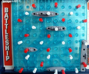
The Battleship® / Coverage Metaphor
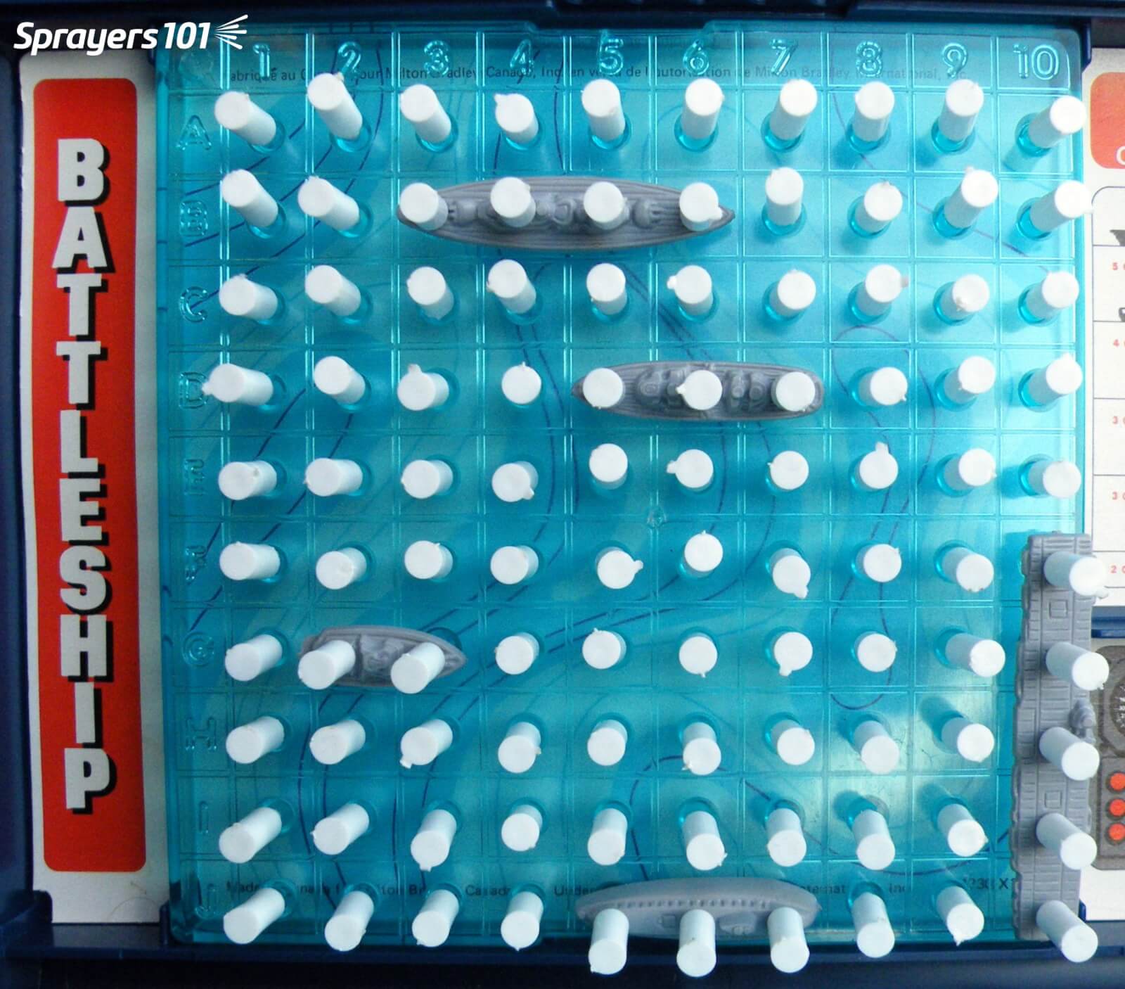
Imagine the boats in this Battleship® game are the insect pests, and the board they’re on is a leaf. The white pegs represent the spray deposits. In this first image, we see 100% coverage and a very high deposit density. Sure, we got every boat, but this is literal and figurative overkill. There’s no need to completely drench the target in order to control most pests. When you spray a target past the point of run-off, you are not adding more pesticide to the target – you are displacing what was already there. The surface will not exceed the concentration of product you sprayed (with the possible exception of mixes that include certain adjuvants). While additional volume can improve coverage to a point, there is a diminishing return.
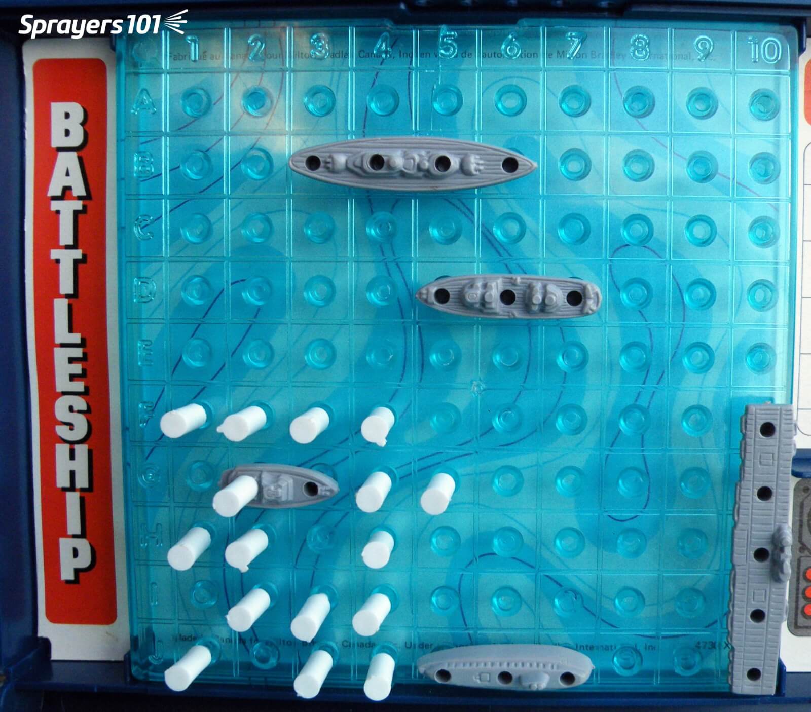
In this second image, we’ve covered about 15% of the target area, which is reasonable. However, note the lack of distribution. You can see that we’ve missed quite a bit of the leaf. If our pretend pests are sedentary and if this was a contact product, then we’ve missed. If this was WSP we would advise the sprayer operator to note how much space there is between the deposits. Could a pest such as an insect or small weed easily fit between the deposits?
In this third image, we are still covering about 15% of the target, but now the spray is distributed more evenly. Some of you are likely noticing that we missed a pest. That observation reminds me of one of my favourite exchanges from the movie “Christmas Vacation” where Clark finally got his house illuminated, but his father-in-law only sees the problems: “The little lights aren’t twinkling.” “I see that and thanks for noticing, Ed.”
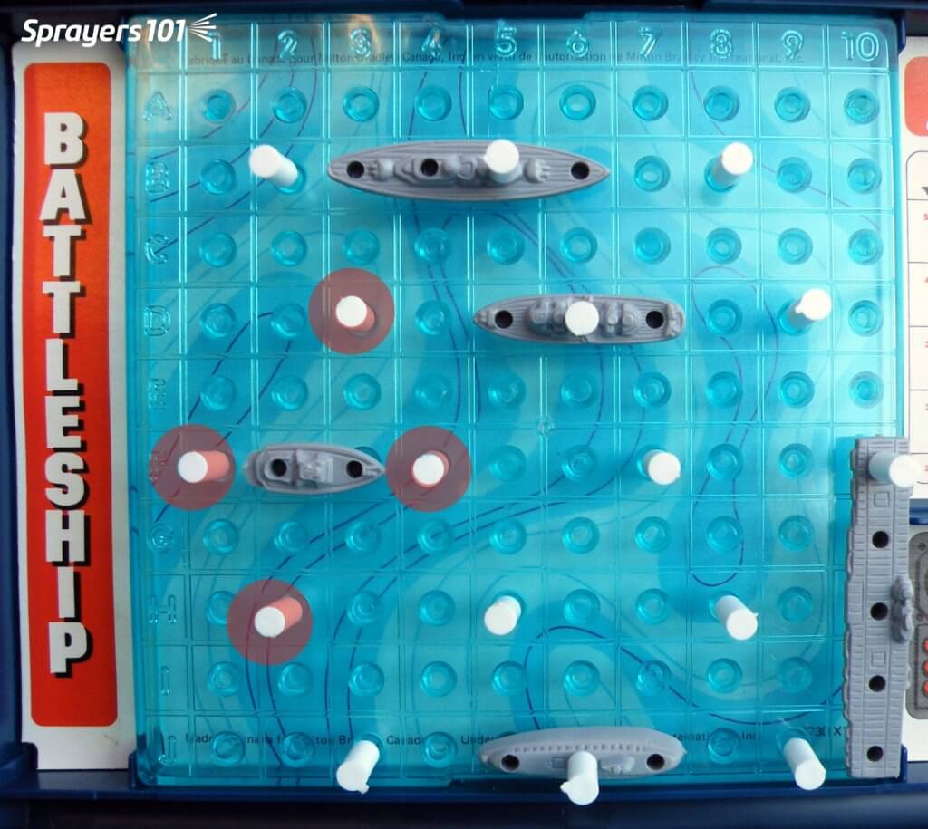
Yes, we still missed a pest, but spraying is playing a game of odds. You want enough spray to increase the odds of controlling a pest, but not so much to waste spray (and money and time). This image represents an ideal coverage situation. If this pest moves, or this pesticide redistributes even a little, it will affect the pest.
Plus, we should not discount the threshold of influence that lies around pesticide residue. Imagine a small circle around each droplet (illustrated here as light red haloes) where active ingredient may redistribute beyond the initial deposit to affect an adjacent pest. Perhaps even more importantly, deposits do not spread on WSP the way they do on actual plant tissue, so WSP always gives an underestimate of the potential coverage.
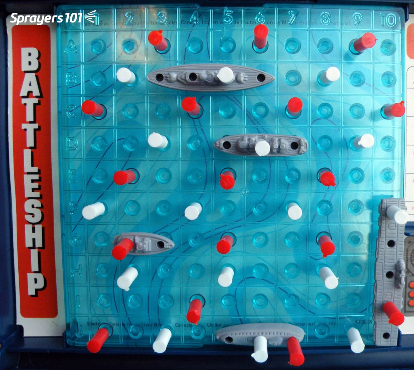
In this last image, we see that red deposits have been introduced. This represents a disease control program where an earlier (white) application retains some residual activity when next application (red) is applied. The second spray application almost never lands on top of the first, giving much more protection on the target. For those keeners out there, note that we got that last pest!
If you Absolutely Need a Number…
So, what if you’ve read all this but still insist on a firm number to define adequate coverage? We’ll reiterate that there’s no universally-accepted threshold of deposit density or area covered. It would be nice if pesticide labels included this information, but they don’t.
We’ll stick out necks out and say that in general practice we see excellent results when we achieve 85 discrete deposits per cm2 as well as 10-15% surface coverage on at least 80% of the water sensitive papers in a spray application. If you can manage this, it should give satisfactory results in most situations.
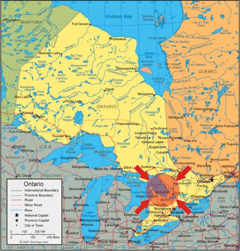
Ontario Agriculture Conference – 2022
For a really in-depth conversation on the topic of coverage, check out our presentation from the 2022 Ontario Ag Conference. We tried to deliver a fun and memorable demo at the end of this presentation to show how different droplet sizes might contribute to coverage. Enjoy.