Calibration should be a regular practice for every operation that uses a sprayer. Part of that process is confirming that each nozzle is operating within the manufacturer’s specifications. This is a must for researchers that adhere to Good Laboratory Practices and for custom operators that sell their services. But we didn’t just fall off the turnip truck… we know nobody else does it. In fact, we’re surprised when we hear an operator HAS checked their nozzle flow.
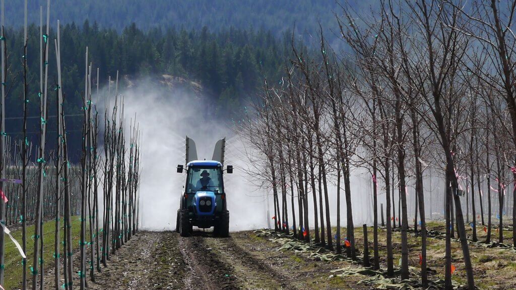
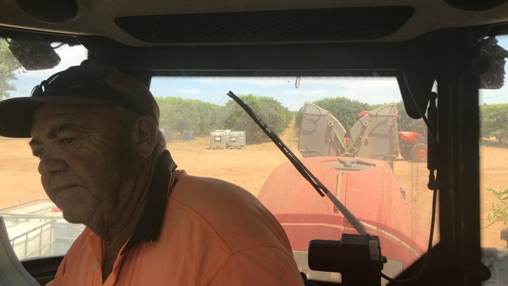
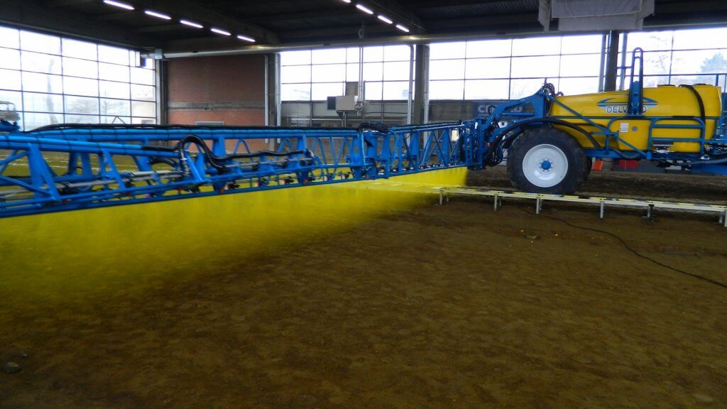
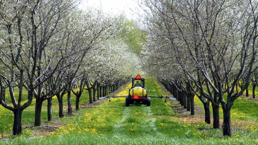
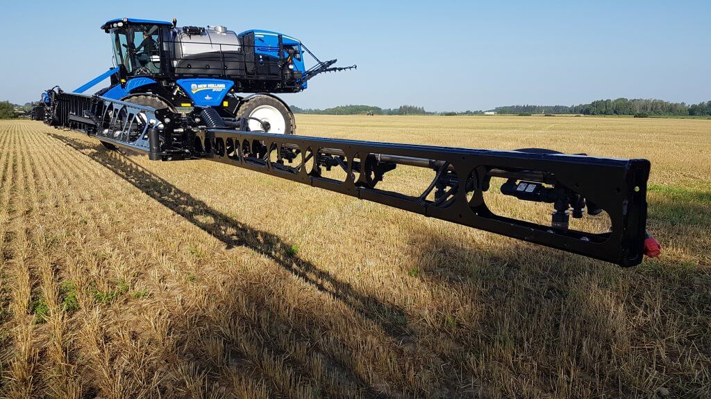
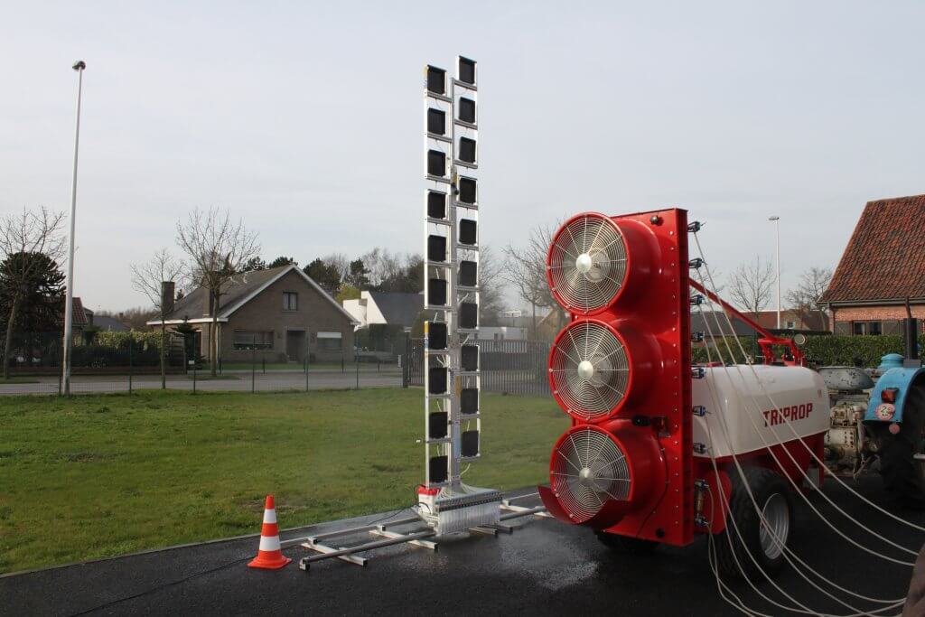
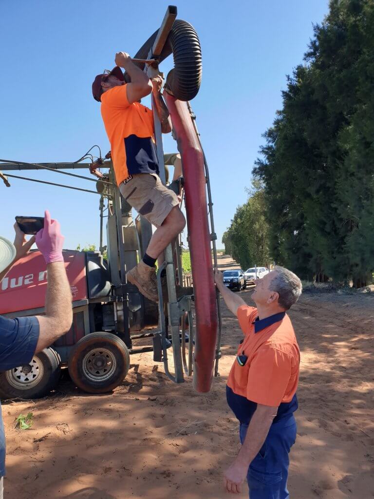
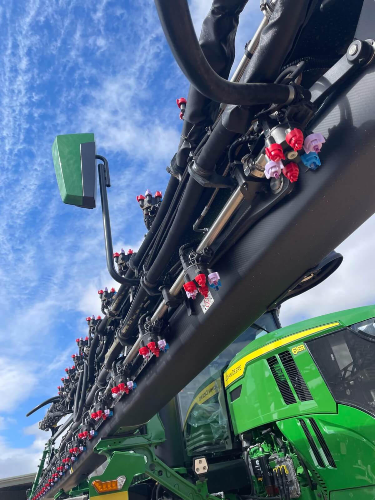
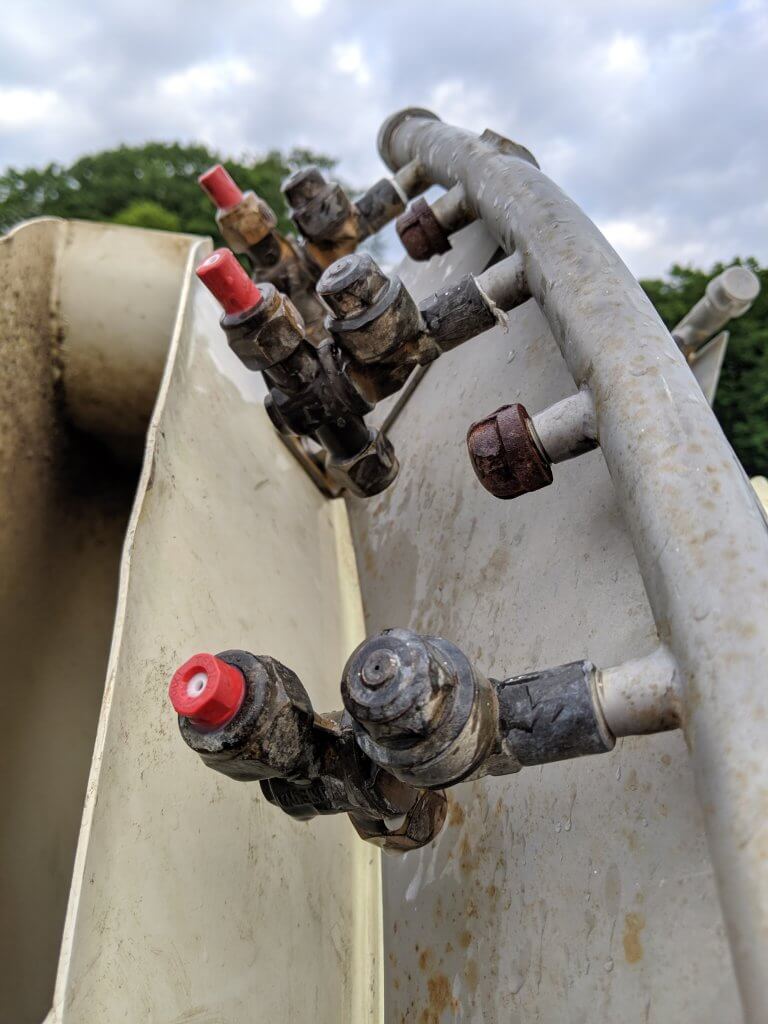
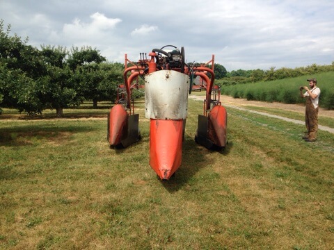
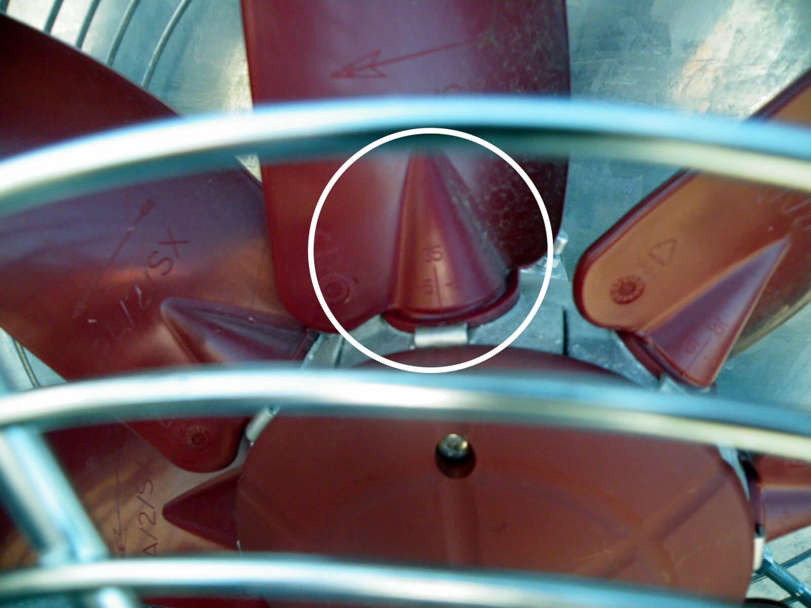
And we get it. It can be awkward and time consuming. A field sprayer with 72 nozzle bodies and three nozzles in each position has a whopping 216 nozzles. A tower-style or wrap-around airblast sprayer has fewer nozzles, but the operator needs a ladder to reach them all and they don’t point straight down, so a tube must be used to guide the spray into a collection vessel.
And when pressed, any operator that does not regularly check their nozzles counters by saying “my tank empties in the same place every time, so why check them?” Even if the sprayer does start to go further on a tank, the operator can speed up or adjust the rate controller to drop the pressure a little.
Fair enough. This isn’t a hill we choose to die on.
But we will say that nozzles worn by even a few percent don’t only cause a change in flow rate, but may indicate a deteriorating spray quality and spray geometry. And, when one (or a few) nozzles are worn and others are not, it’s the same as when a single nozzle is plugged – the operator won’t be able to tell from the cab because the rate controller tends to mask the problem. And, if using PWM to apply a simultaneously reduced broadcast rate, perhaps the issue is amplified? All of this impacts coverage uniformity.
We’ll get off our soapbox now.
Over the years we’ve encountered many methods for determining a nozzle’s flow rate. We wanted to try each of them and characterize their accuracy, precision, time required, and ease of use. This is not a ranking where we wanted to find “The Best” method. The best method depends on your situation. If you’re a researcher, then accuracy and precision may trump time and expense. If you’re a custom applicator, then perhaps time is the critical factor. And if it’s your own operation, perhaps expense matters most. It’s up to you.
Method
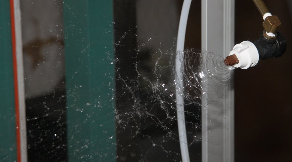
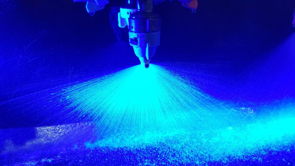
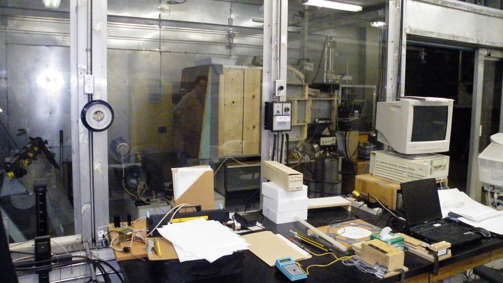
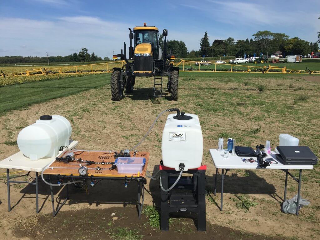
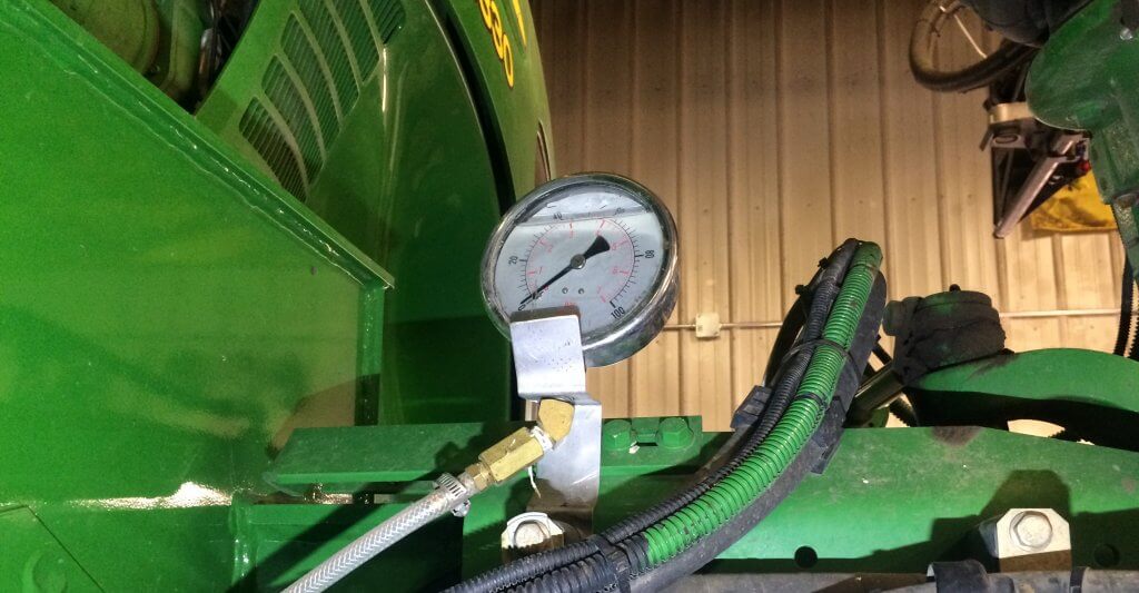
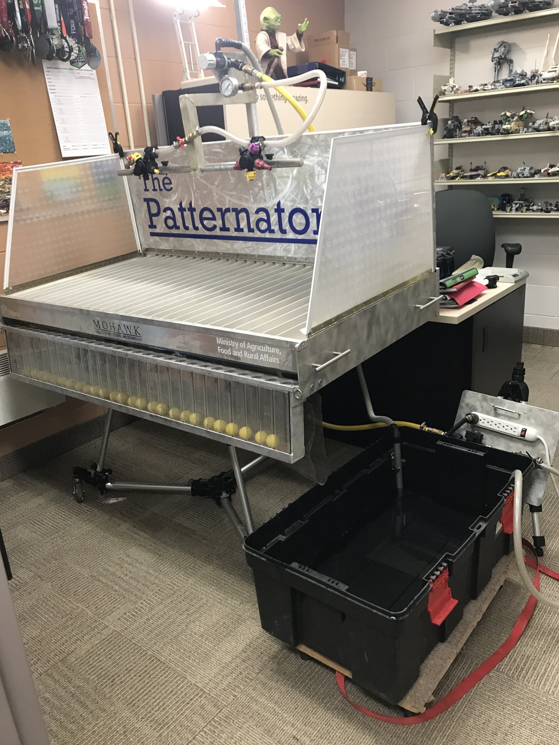
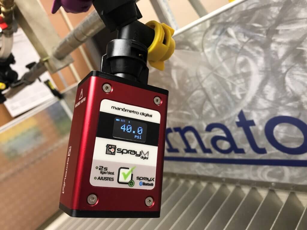
The following tests were performed on a spray patternator table. A single nozzle was operated by a ShurFlo 2088-594-154 positive displacement pump. Pressure was set using a bypass regulator and an analog pressure gauge, confirmed by a SprayX digital manometer positioned under the nozzle body via a splitter. Room temperature water was used.
We tested ten nozzle flow rate measurement systems. There are others out there, but we limited the selection to farmer-oriented systems and not those used in mandatory government inspections.
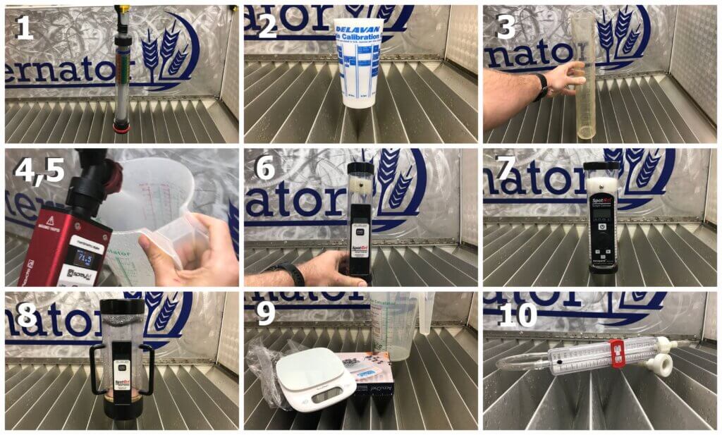
- Billericay Flowcheck
- Delavan Calibration Cup
- Graduated Cylinder
- Greenleaf Calibration Pitcher
- SprayX SprayFlow Turbo
- SpotOn SC-1
- SpotOn SC-2
- SpotOn SC-4
- Weighed Output
- Lurmark McKenzie Calibrator
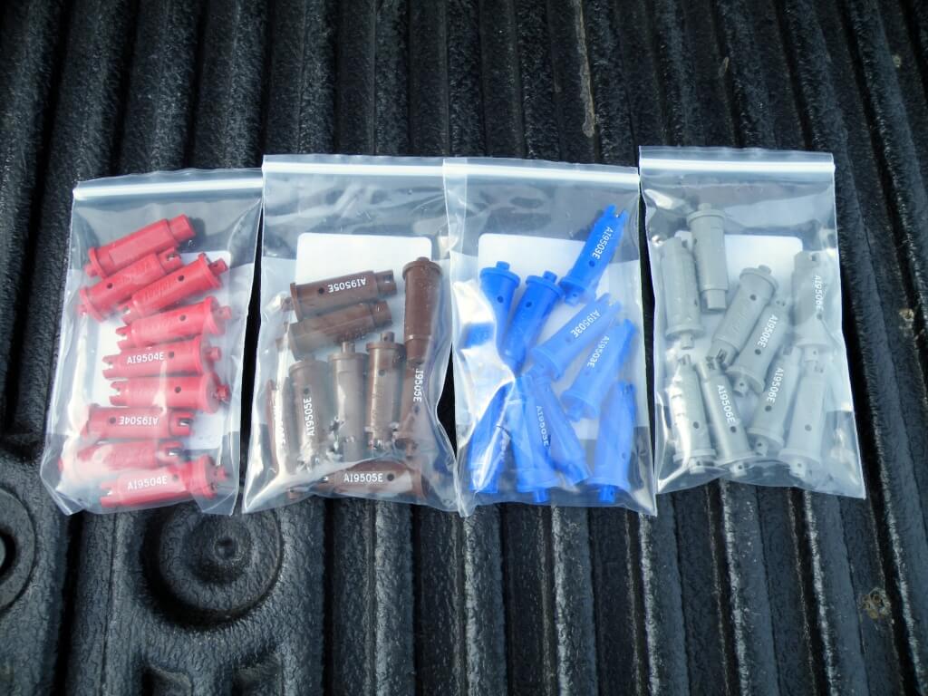
Three samples were taken from a new TeeJet XR8004 at ~40 psi and three samples taken from a new TeeJet AIXR11004 at ~70 psi. An exception was made for the Billericay Flowcheck which specified 43.5 psi (3 bar) for all sampling. All systems were emptied or dried as much as their design permitted between samples.
All data was converted to gallons per minute and the flow measured was compared to the calculated flow for the nozzle and pressure used. For example, if the manometer read 38 psi for the 8004, then the formula 0.4 x (38 psi ÷ 40) 0.5 gives us a calculated flow of 0.39 gpm. If the method reported 0.41 gpm, then it would be off by +5.1%.
Results
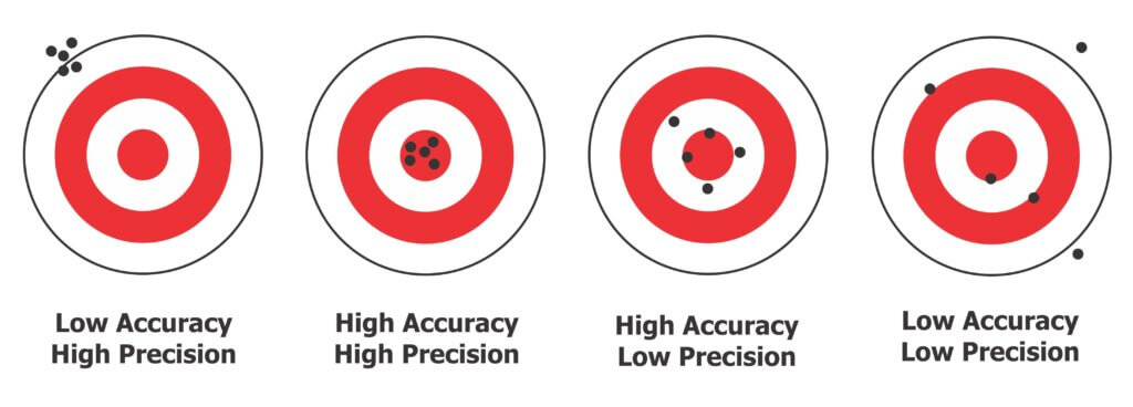
Consider the accuracy and the precision of each system when you review the results. Remember that precision means you get the same result with very little variation while accuracy means that on average you get the correct result. And, for context, remember that most recommend changing a nozzle when it is 10% more than the ideal flow rate. We prefer 5%, and if three or more nozzles are off spec, replace them all as a batch because they’re likely all very close. Compared to most spraying costs, a set of nozzles is not worth quibbling about. Some operators just change them annually and don’t bother with testing at all.
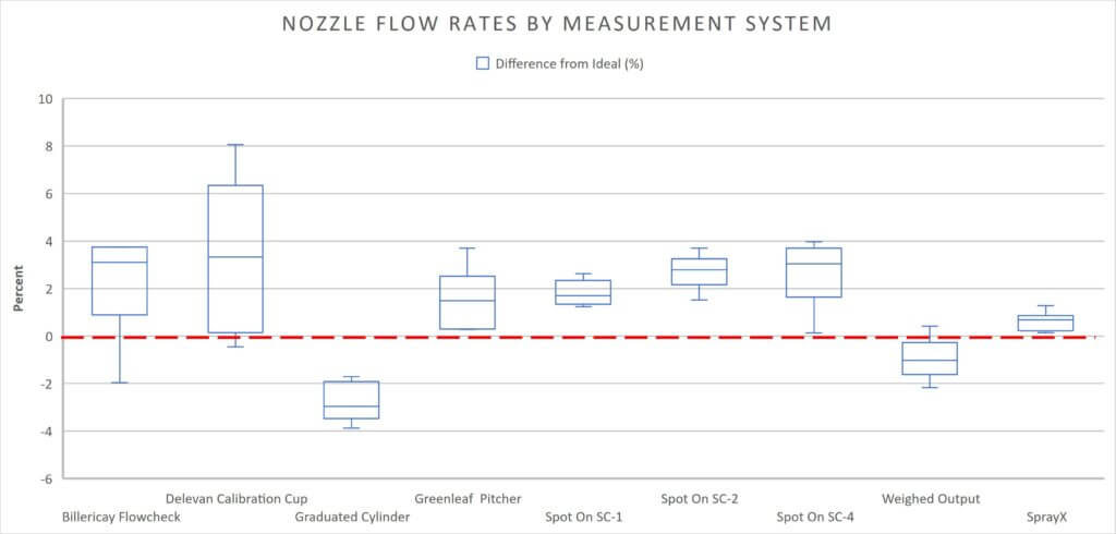
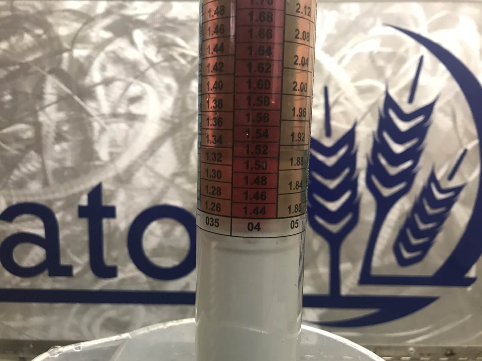
Billericay Flowcheck: This is a passive measurement system. You must select the nozzle size on the bottom of the collector and suspend the unit from the nozzle body. It’s designed for a horizontal boom and you’d have trouble using it with any other sprayer. You also have to set the pressure to exactly 43.5 psi (3 bar). While fairly accurate, it spanned about +/-2.5% off ideal. You have to read from the right scale, which in this case was red and rather difficult to read because of the low contrast. It took about two minutes to reach equilibrium for each reading and a lot of liquid is lost during the process.
Delavan Calibration Cup: This small, one-handed plastic cup had a scale printed on the outside. We were limited to a 15 second collection because of how quickly it filled. Some spray was lost to mist and bounce and we used the “Fluid Oz” scale to get the highest resolution from the measurement. It took less than a minute to collect and read from the cup, but had the lowest precision and accuracy.
Graduated Cylinder: There was little or no mist or bounce from escaping spray during collection. Our 1,000 ml graduated cylinder took 30 seconds at 40 psi and 20 seconds at 70 psi to fill making it roughly one minute per reading. A few light taps removed bubbles and once the liquid settled we could read the level. This must be performed on a level surface (in our case we used the digital level app on our iPhone). This was a very precise method, varying by less than 2%, but it wasn’t very accurate. We may have introduced error when reading the meniscus (always read from the centre) or perhaps the plastic distorted over time and affected accuracy. It may be difficult for most people to get a high quality, scientific-grade graduated cylinder.
Greenleaf Calibration Pitcher: The pitcher had multiple scales but once again we used fluid ounces because it had the highest resolution. With the highest capacity, we were able to collect for an entire minute. Despite holding the vessel at different angles and distances, we lost a lot of spray to mist and bounce and the nozzle body was beaded with water at the end of each trial. After tapping the vessel to remove bubbles and reading on a level surface, it took about 1.5 minutes per sample and averaged an average 3% more than the calculated ideal flow rate.
Innoquest Spot On Digital Calibrator: We’ll discuss all three Spot Ons together. The Spot Ons were a game-changer in North America when they first came out. You can read a peer-reviewed article about the SC-1 by Dr. Bob Wolf et al. published in 2015 in the Journal of Pesticide Safety here. The SC-2 is a new version of the SC-1 with added digital features that allow the user to calculate gallons per acre and it indicates tip wear based on the 10% industry standard . The most important improvements were a reduced sensitivity to foam and a thicker foam diffuser to reduce the chance of errors. The SC-4 works exactly like the SC-1, but has a larger capacity intended for high flow rate nozzles (e.g. hollow cones on an airblast sprayer). In each case, the Spot On will report in several units, and must be held steady under the nozzle flow (i.e. not moved during reading). The SC-1 and 2 took less than 12 seconds for each reading and the SC-4 took closer to 30. The SC-1 and SC-2 were relatively precise but read consistently higher than the calculated flow rate. This may be an artefact given that the units only read to 2 decimal places and this may have exaggerated any error. The SC-4 was the least accurate and precise of the three. The Spot Ons were the fastest and easiest to read of the methods used.
Weighed Output: This method is based on the fact that 1 ml of water weighs one gram. Spray was collected for 30 seconds and weighed on a new, $25 CAD digital kitchen scale, which was tared (i.e. the weight of the vessel subtracted from the overall weight). While subject to errors from manual timing, it has the merit of removing the challenge of reading a meniscus and it’s relatively inexpensive. This method was precise and relatively accurate compared to the other methods used. It took about a minute per sample.
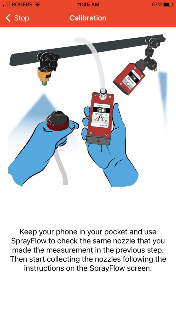
SprayX SprayFlow Turbo: This was the most sophisticated method we used. The kit comes with a digital manometer, a flowmeter and a digital scale. It works though a smartphone app (screenshot below). You first have to set up a virtual sprayer, informing the app how many sections and nozzles will be tested. Then you must calibrate the flow sensor by taking three measurements versus a weighed output to eliminate possible variations caused by the nozzle, pressure, temperature, and the density of the liquid. The app walks the user through each step. This method took the most time to set up (easily 10 minutes). However, once it was set up, each nozzle could be tested in less than 30 seconds apiece. This method was the most accurate and precise, but the price may place it out of reach for the typical user.
Lurmark McKenzie Calibrator: This method is not reported in the box-and-whisker plot because there were significant problems that prevented accurate readings. It was difficult to get a seal over the nozzle and the floater ball would either stick or fluctuate. After several attempts, this method was abandoned.
Conclusion
In order to test if a process, or a thing, is occurring or produced within acceptable limits, we need a detection system with a high enough resolution. In manufacturing (e.g. factory production) this is an essential requirement in quality assurance. Let’s consider a +10% deviation from the nozzle’s ideal flow rate to be our indication that a nozzle needs to be replaced. We need a measurement system with an appropriate scale and one with sufficient precision to ensure we don’t get a false reading. Based on our data, I would suggest all systems reviewed, save the measurement cup, are viable. Even if we elect to use a more stringent rejection threshold of 5%, some systems are more precise than others (i.e. less variability), but all but the cup should still be sufficient.
What’s the penalty for not testing, assuming we’re not talking about significantly deviant nozzles? Let’s say, for example, we are not using a rate controller and we are applying 20 US gpa at 12 mph using 72 nozzles on 20″ centres. Our boom would have to spray 58.2 gpm, which means each nozzle would have to emit 0.81 gpm. If those nozzles sprayed 5% more than intended, we’d be spraying 21 gpa instead of 20 gpa. That means for a 1,200 gallon sprayer, you’d do 57 acres instead of 60. We would have the same result if we dropped from 12 mph to 11.45 mph, which is about 5% slower. Maybe that’s a big deal for your operation, or maybe not. For most, 5% is well within the typical error inherent to spraying. Then again, perhaps it’s more important to know that each nozzle is performing in a manner similar to its neighbours to ensure the highest degree of coverage uniformity.
Ultimately, it is important to ensure you’re as efficient as possible, and that means understanding what your nozzles are doing so you can decide if-and-when it’s time to replace them. Pick whichever method makes it easiest for you to justify testing your nozzles and do it at least once a year when you take your sprayer out of long term storage.
Thanks to all the companies that donated or loaned their calibrators to make this article possible.