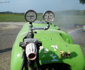
The role of pressure is often underappreciated in spraying. Many airblast operators (still) don’t use rate controllers, so the only way to monitor sprayer pressure is using a single liquid-filled pressure gauge located near the pump… and it may not be trustworthy. An inaccurate pressure gauge may cause you to spray more or less product than you intended. That translates to wasted resources and potentially higher residue levels. Conversely, spraying less than intended may lead to reduced efficacy and the need to re-apply. Many operators use budget pressure gauges on their sprayers and have never tested or replaced them.
Testing pressure gauges
Here are a few clear indications that your pressure gauge should be retired:
- Gauge has an opaque or unreadable face
- Mineral oil leaking or mostly gone
- Needle does not rest on zero pin when sprayer is not under pressure (it has likely spiked)
Sometimes a gauge is not obviously in need of replacement. To test it, you need to apply a known pressure to see if it is reading accurately. One way to do this is using a commercial manometer.
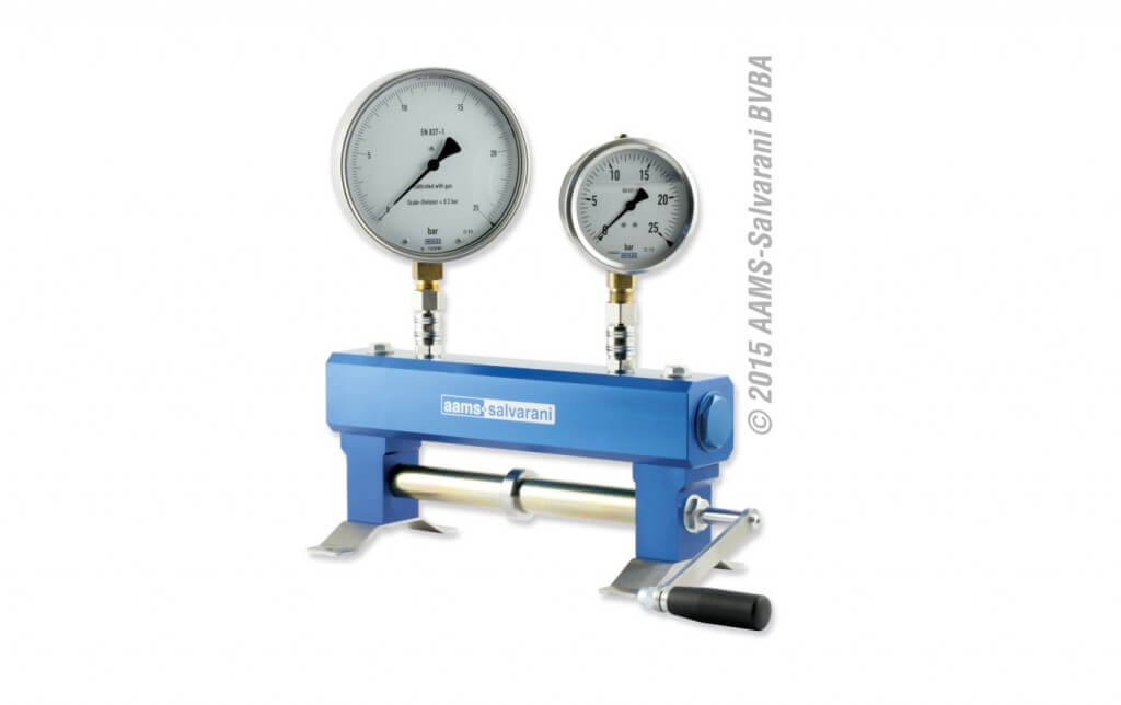
These systems work well, but they can be an expensive proposition if you only use them once in a while. In a past sprayer workshop, one participant had a great suggestion for testing gauges. His idea was to use an air compressor (which most farms have) and some simple plumbing to create a homemade manometer. Be sure to vent the gauges before testing.
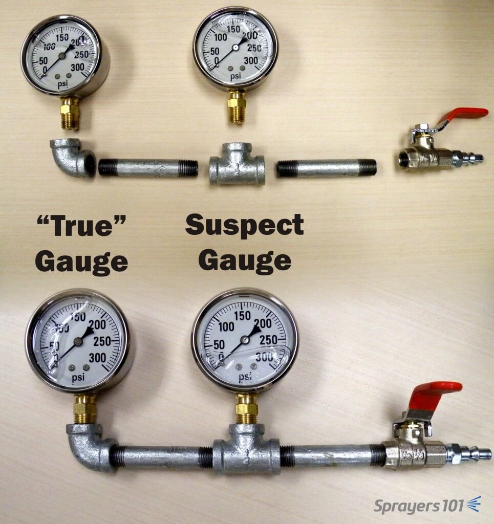
This tool allows you to test your suspect gauge (set in the tee) against an accurate gauge (set in the elbow) for less than $75.00 CAD. Construct your own “Pressure Gauge Tester” using the following parts (valve optional):
| Part | Approx. Price (CAD) |
| ¼” by 3” Galvanized nipples (x 2) | $3.50 |
| ¼” Galvanized 90º elbow | $3.50 |
| ¼” Galvanized Tee | $3.50 |
| ¼” Ball valve (threaded) | $10.00 |
| *Plug Air Connector (A over ¼”) | $4.00 |
| Teflon pipe tape | $3.00 |
| †300 psi liquid-filled gauge | $40.00 |
| *Depending on the quick-connect fitting on your compressor | |
| †The range of the accurate gauge should match your existing gauge. The range of your existing gauge should be twice as much as your typical operating pressure. |
As a public service announcement, be aware that many budget, liquid-filled gauges are inaccurate right off the shelf. A 5% variance is typical. When replacing a worn gauge, or buying the “accurate” test gauge for your homemade manometer, buy a few and save the receipt. Test them in different combinations to ensure they all agree with one another. Return the extras and let the dealer know if you discover an inaccurate gauge. I’m sure they won’t put it back on the shelf for the next person… *ahem*.
Gauges should be rated twice as high as your average operating pressure. For example, if you typically spray at 150 psi, your should have a gauge rated up to 300 psi. That way, you can see small changes in pressure more clearly. Plus, if your needle is pointing straight up, a quick glance confirms the ideal operating pressure.
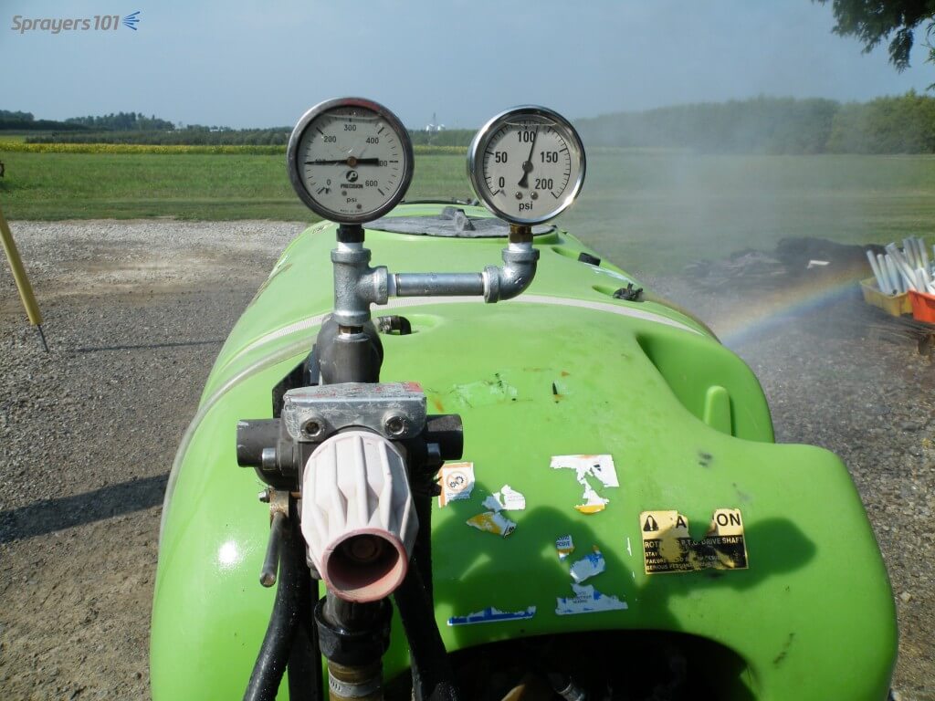
Another way to confirm pressure gauge accuracy is to install a second in-line. They’ll keep one another honest. This may be difficult if the gauge set into a molded plastic tank, or located under the chassis next to the pump where it is not visible from the tractor.
Measuring and Correcting for Pressure Drop
Boom pressure can sometimes be less than the desired operating pressure (a phenomenon known as “pressure drop”) and must be accounted for. Pressure drop is affected by hose diameter, hose fittings, and the distance from the pump. You’ll find it at the far ends of boom sections on field sprayers and it’s an issue that plagues many low-pressure, tower-style sprayers. Dress appropriately because you’re going to get wet performing this diagnostic.
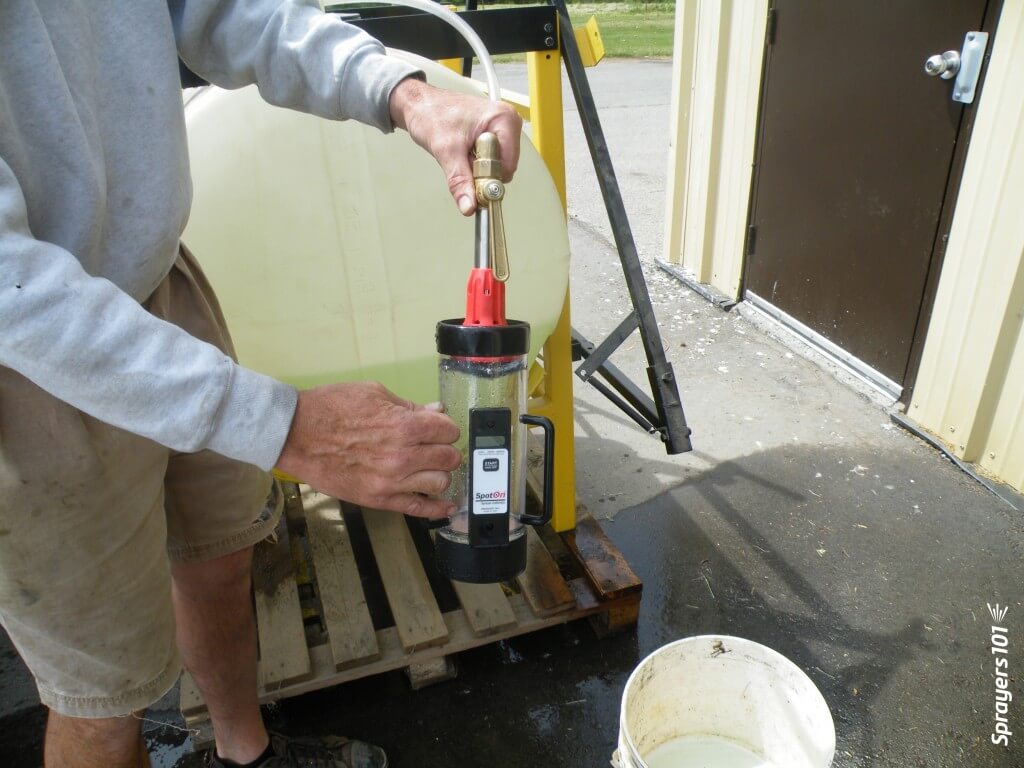
- Fill a clean sprayer about half-full with water.
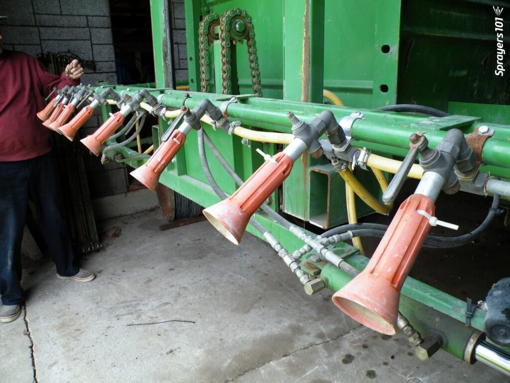
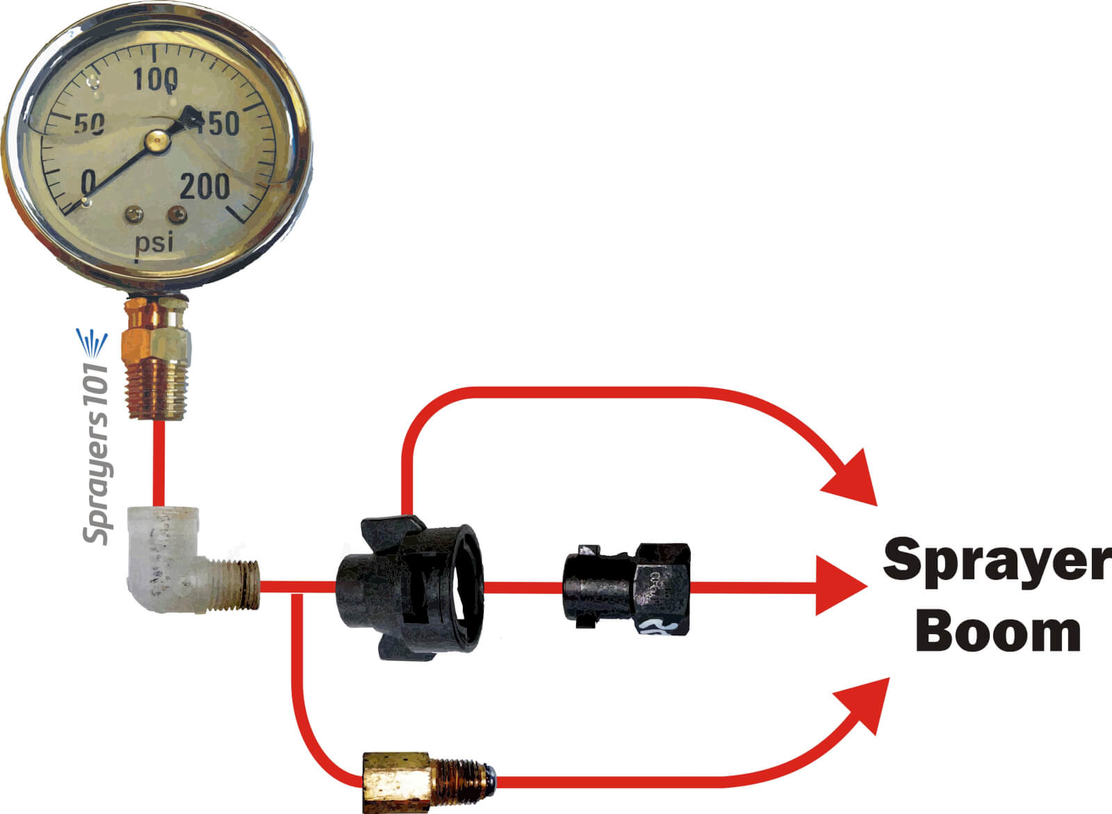
- Install a liquid-filled test gauge in the highest nozzle position of one of the booms. The image below shows how the nozzle cap or entire nozzle body may need to be removed for this step. For Metric fittings, contact your sprayer dealer – they can be hard to find.
- With the tractor parked, bring up the rpms and get the lines to the desired operating pressure.
- Open the boom(s) and measure the pressure at the nozzle farthest from the pump. All nozzles on all booms should be open during this test. That’s why you are wearing PPE.
- For positive displacement pumps, adjust the main pressure regulator until the test gauge reads the desired pressure. For centrifugal pumps, it is possible to make small changes to the pressure, but more important to note any pressure differential for later considerations regarding nozzle output and spray quality.
Switching between multi and single boom operation
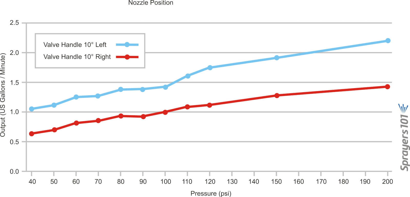
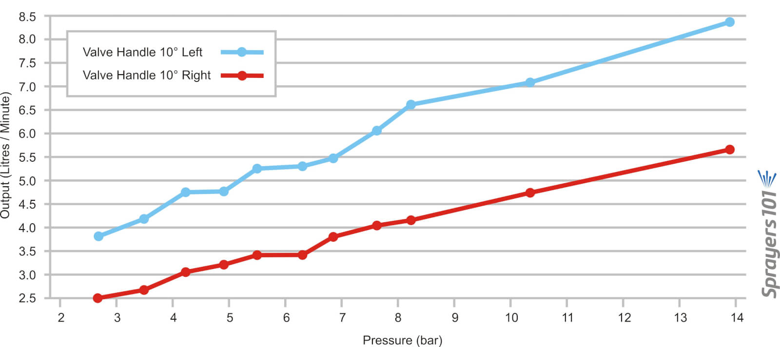
When sprayers that employ a positive-displacement pump are switched to one-sided operation (E.g., border spraying or during turns), the pressure can change considerably. Most units will experience a pressure increase, thereby increasing the boom output. This is typically an indication of a faulty relief valve, which is positioned between the pump and nozzles. It’s actuated by a spring-loaded piston or diaphragm, opening and closing in response to changes in pressure. The operator sets the desired pressure and any additional pressure forces the valve open, diverting excess flow back to the tank via a bypass.
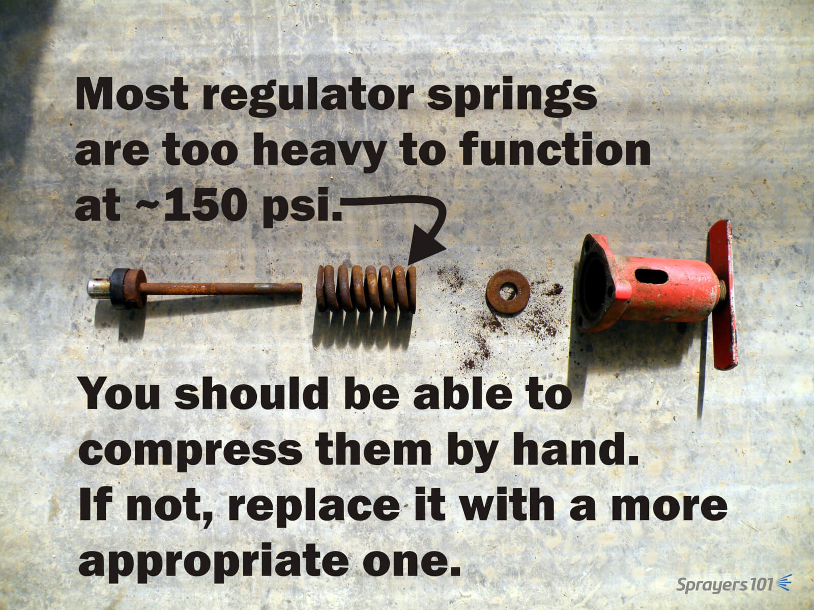
This problem can be greatly reduced by properly sizing the regulator (specifically the spring) to the typical operating pressure. Many sprayers come equipped with regulator springs matched to the maximum pressure range of the pump (often 600 – 900 psi). These springs are unable to respond to changes when operating at lower pressures (E.g., 100-200 psi, which is typical of applications to moderately-sized canopies).
The springs are so stiff that the liquid pressure is unable to act on the spring and the valve essentially acts as a flow control (throttling) valve rather than a pressure control valve. Liquid pressure is difficult to control using a throttling valve; it is unable to compensate if the tractor engine speed drops while driving uphill and sprayer output is subsequently reduced. Further, this phenomenon can cause pressure gauges to spike.
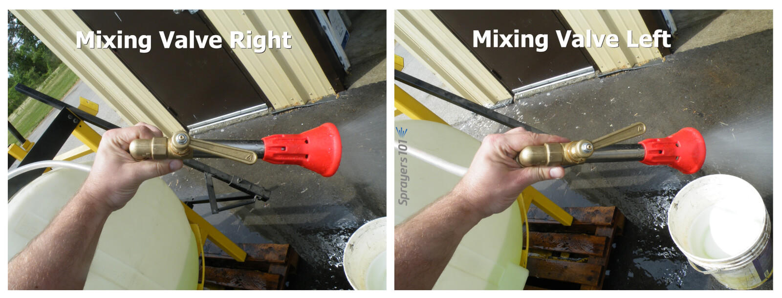
Some sprayer designs attempt to compensate for excess flow during single-boom operation. They employ an additional throttling valve to shunt the volume that would normally would be spraying out through the closed boom. The result is that the pressure should remain constant when a single boom is shut off. If your sprayer has this feature, here’s how you set the valve:
- With PTO at application speed and both booms open, adjust regulator to calibrated operating pressure.
- Close one boom.
- If pressure increases, open throttling valve to achieve calibrated operating pressure. If pressure decreases, close throttling valve to achieve calibrated operating pressure.
- Repeat process for the other boom, and find a compromise position for the valve.
Some operators elect to remove the handle from the throttling valve once it is set so they don’t accidentally bump it later. That’s fine, but further adjustments may be required when transitioning between dilute and concentrated volumes, so don’t lose the handle.
Here’s an oldie-but-a-goodie filmed in New Hampshire in June, 2014. It’s something to keep in mind when you’re getting your sprayer ready for spring service. Thanks to Chazzbo Media and Penn State Extension for making an unscripted and spur-of-the-moment concept into a polished video.