Category: Speciality Sprayers

Main category for all sprayers that are not horizontal booms

Spray Coverage in Field Tomato

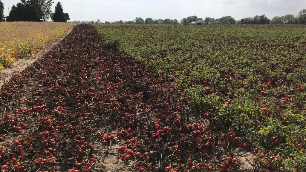
Spraying field tomato is difficult – period.

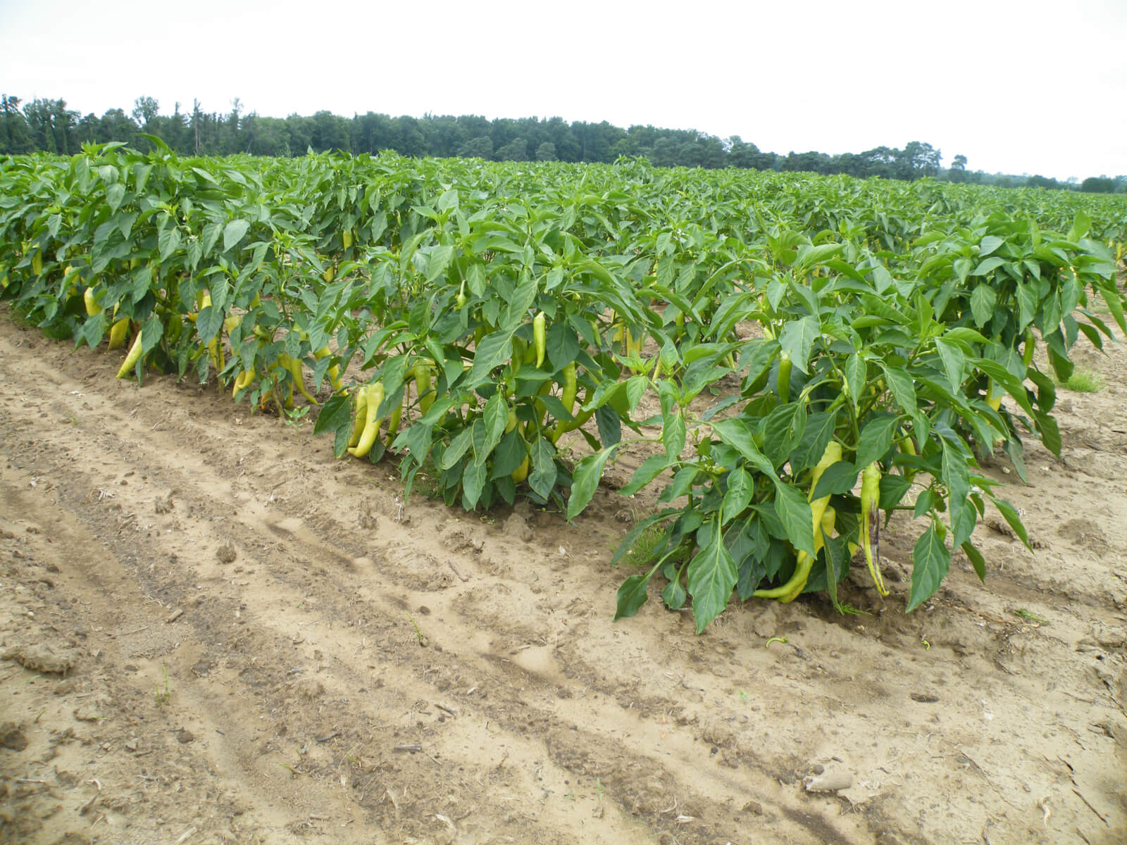
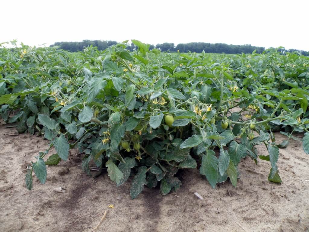
In Ontario, early variety tomato canopies get very dense in July. The inner canopy is relatively still, humid, cool and a perfect environment for diseases such as late blight. It is challenging to deliver fungicides to the inner canopy and this can lead to inadequate disease control. Matters are slightly improved as the fruit grows and pulls the canopy open, and staked tomatoes might allow for the use of directed sprays, such as drop arms in staked peppers. But, there’s no getting around it – from a droplet’s perspective, it’s tough to get through the outer canopy.

DSCF0002 — Imagine you are a spray droplet trying to get inside this canopy.

Study 1 – Qualitative Observations

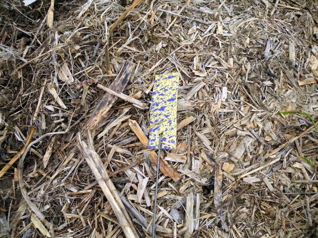
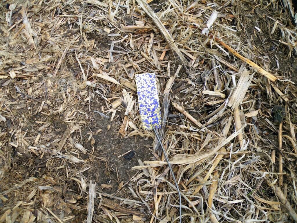
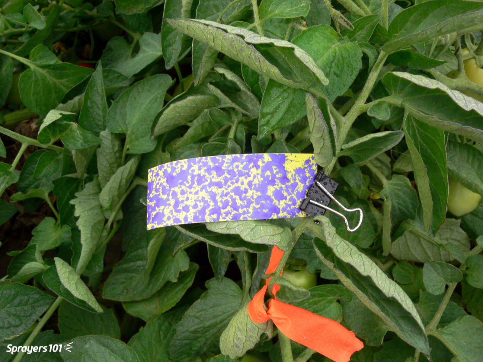
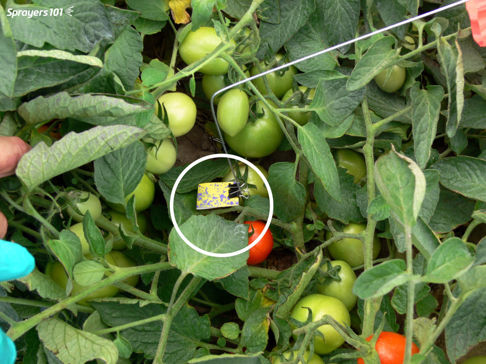
In August, 2011 we worked in a market garden operation in Bolton comparing the spray coverage from four different nozzle configurations. We used the growers typical spray parameters: a travel speed of 4.5 km/h (2.8 mph), an operating pressure of about 4 bar (60 psi), a boom height of 45 cm (18 in) above the ground, and a sprayer output of 550 L/ha (~60 gpa). To monitor spray coverage, water sensitive paper was placed face-up in the middle of the tomato canopy. This diagnostic tool turns from yellow to blue when contacted by spray.

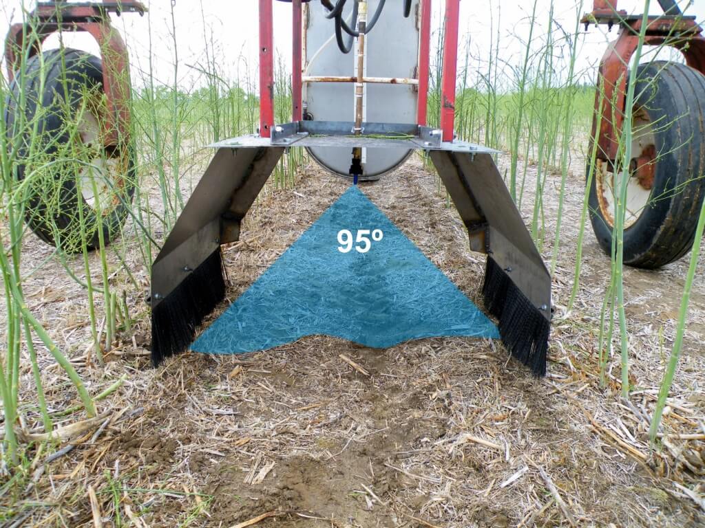
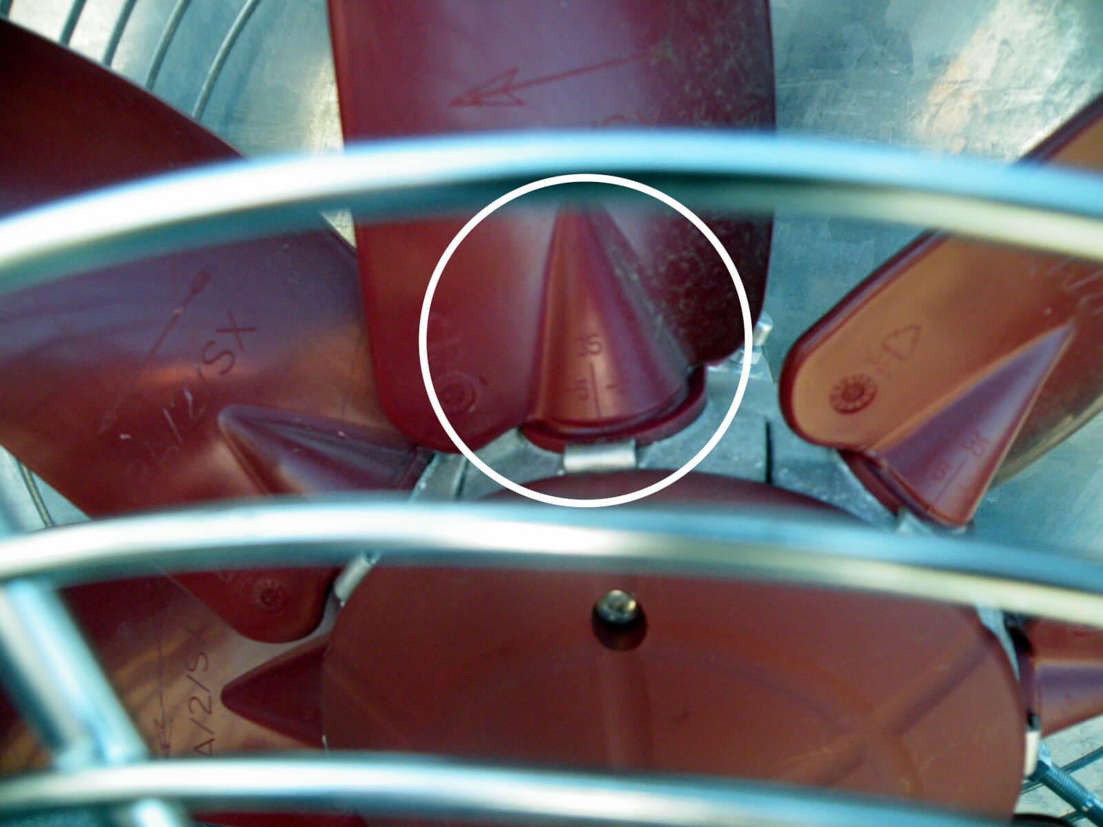
Water-sensitive paper at top of tomato canopy - easy to hit. — Water-sensitive paper at top of tomato canopy – easy to hit.

This particular sprayer was equipped with an air assist sleeve that blew a curtain of air into the canopy at about 100 km/h (65 mph) as indicated by an air speed monitor placed at the air outlet. When properly adjusted, air-assist booms have a number of benefits:

They part the outer canopy giving spray access to the inner canopy.
They rustle leaves to expose all surfaces to spray.
They permit the use of smaller droplets, which are more numerous and adhere to vertical surfaces, by entraining them and reducing drift.
They extend the spray window by permitting the applicator to operate in slightly higher ambient wind speeds.

Boom sprayer with air assist sleeve operating.

We sprayed using the four different nozzle configurations, with and without air assist. Our goal was to make qualitative assessments (Good, Moderate, Poor), and here’s what we observed:

Nozzle Type / Sprayer Output	With Air Assist	Without Air Assist
80 degree flat fans /~550 L/ha (60 g/ac)	Good coverage in upper canopy Poor / Moderate canopy penetration Low drift	Good coverage in upper canopy Poor canopy penetration Moderate drift
80 degree air induction flat fans /~550 L/ha (60 g/ac)	Inconsistent upper canopy coverage Poor canopy penetration “No” drift	Inconsistent upper canopy coverage Poor canopy penetration “No”/Low drift
TwinJet dual 80 degree flat fans /~550 L/ha (60 g/ac)	Good coverage in upper canopy Poor / Moderate canopy penetration Moderate Drift	Good coverage in upper canopy Poor canopy penetration Moderate/High drift
Hollow cones /~750 L/ha (80 g/ac)	Good coverage in upper canopy Moderate canopy penetration Low drift	Good coverage in upper canopy Poor canopy penetration Very High drift

The air induction nozzles performed poorly. Their Coarse/Very Coarse droplets impacted on the outer canopy, created run-off and resulted in very little canopy penetration. Medium droplets produced by twin fans and conventional flat fans were both inconsistent with inner-canopy coverage, but some advantage may have been observed with air assist. The TwinJets contributed to higher drift (likely because they were too high off the canopy) but otherwise produced coverage similar to the conventional flat fans. From these observations, the convention that spray shape (e.g. cone, fan, twin) has little or no impact on broadleaf canopy penetration holds true.

Acceptable spray coverage deep in canopy (harder to hit) using hollow cone nozzles. — Acceptable spray coverage deep in canopy (harder to hit) using hollow cone nozzles and air assist.

After inspecting the papers deep in the canopy, we were surprised that air assist did not obviously improve canopy penetration. It did seem to help, but it wasn’t a slam-dunk. This may be because finer droplets (<50µm) are not easily seen on water sensitive paper. It might also be because we did not calibrate the air speed to the canopy: too little air and spray impacts on the outer canopy, while too much air forces leaves out of the way and spray is blown into the ground. It was obvious that drift was greatly reduced, so logically the spray had to have gone somewhere – we can only assume it entered the canopy.

The best results were achieved with hollow cones and air assist. Theoretically, smaller droplets should improve the potential for coverage by sheer number, but they slow quickly and are easily blown off course. Winds were only about 5 km/h (3 mph) during the trials. Had they been higher, the no-air-assist condition would have resulted in poorer canopy coverage. While we feel the air assist improved inner canopy coverage, we attribute much of the performance to the spray volume of 750 L/ha (80 gpa), which was significantly higher than we used with the other nozzles. When we attempted lower volumes using the hollow cones (not shown) the inner canopy coverage was greatly compromised. Higher volumes are a demonstrated means for improving canopy penetration, so this observation is consistent with what was expected.

The 2011 trial suggested that hollow cone tips used with high volume and air assist, improved canopy coverage and penetration. They are, however, very prone to drift and their use is not recommended without an air assist sleeve to counter the spray drift. Spray volumes over 500 L/ha are highly recommended.

Study 2 – Quantitative Observations

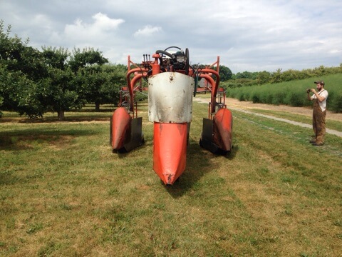
In July, 2016 we ran another study in Chatham-Kent. This operation was concerned about spray drift and recently changed from Hardi hollow cones on 25 cm (10″) centres to TeeJet Turbo TwinJets on 50 cm (20″) centres. They wanted to know if they had improved their coverage. We decided to test four nozzles at similar driving speeds and volumes.

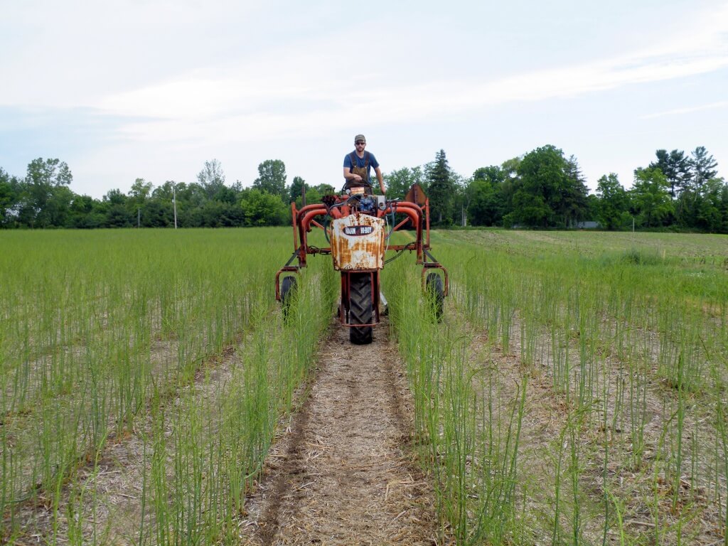
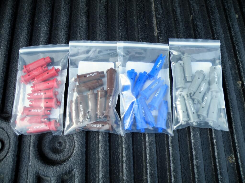
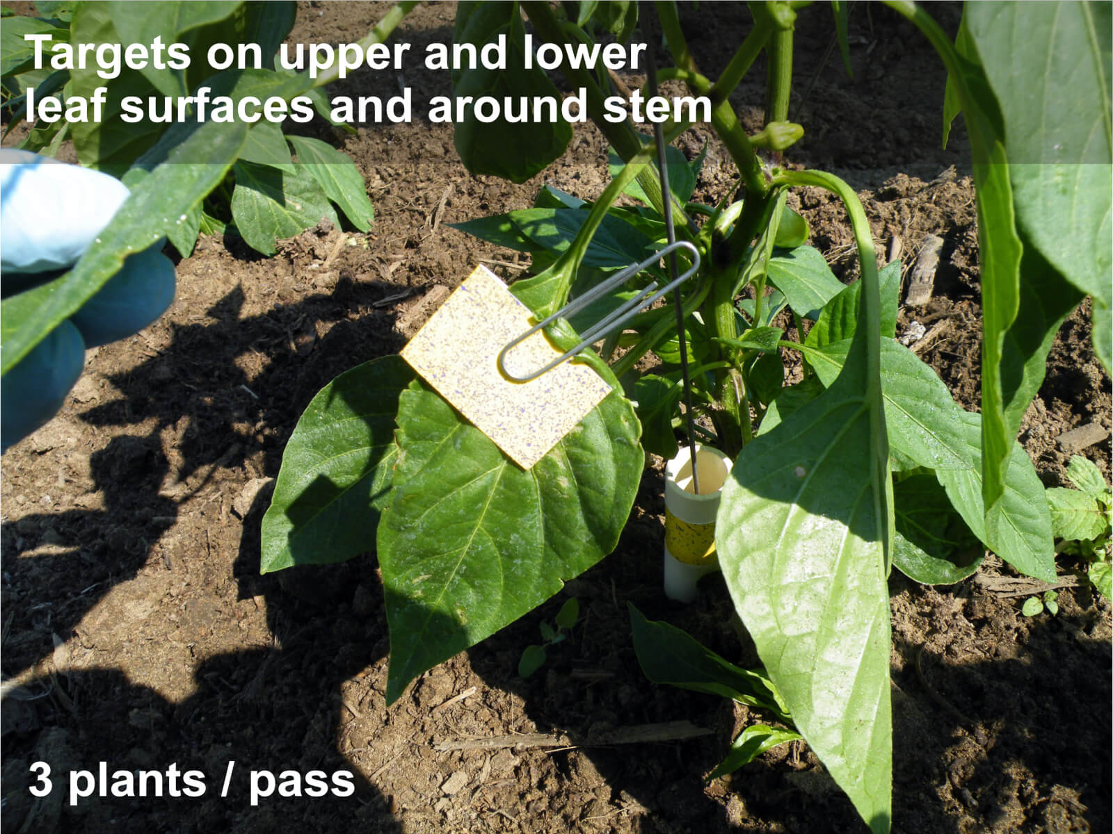
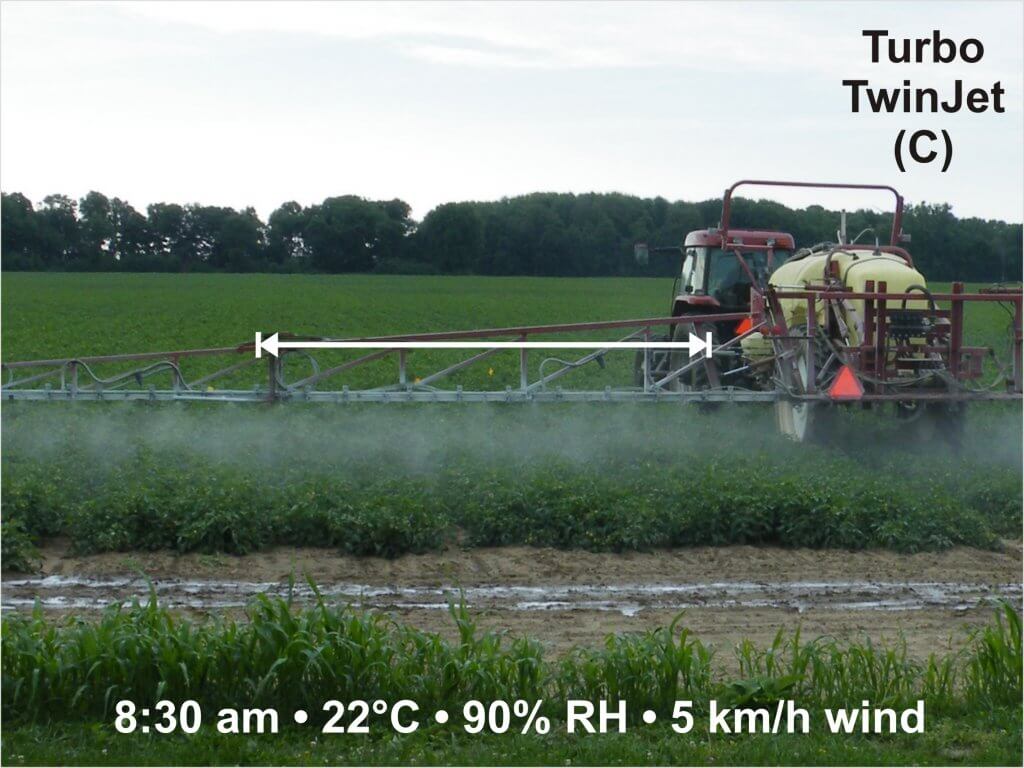
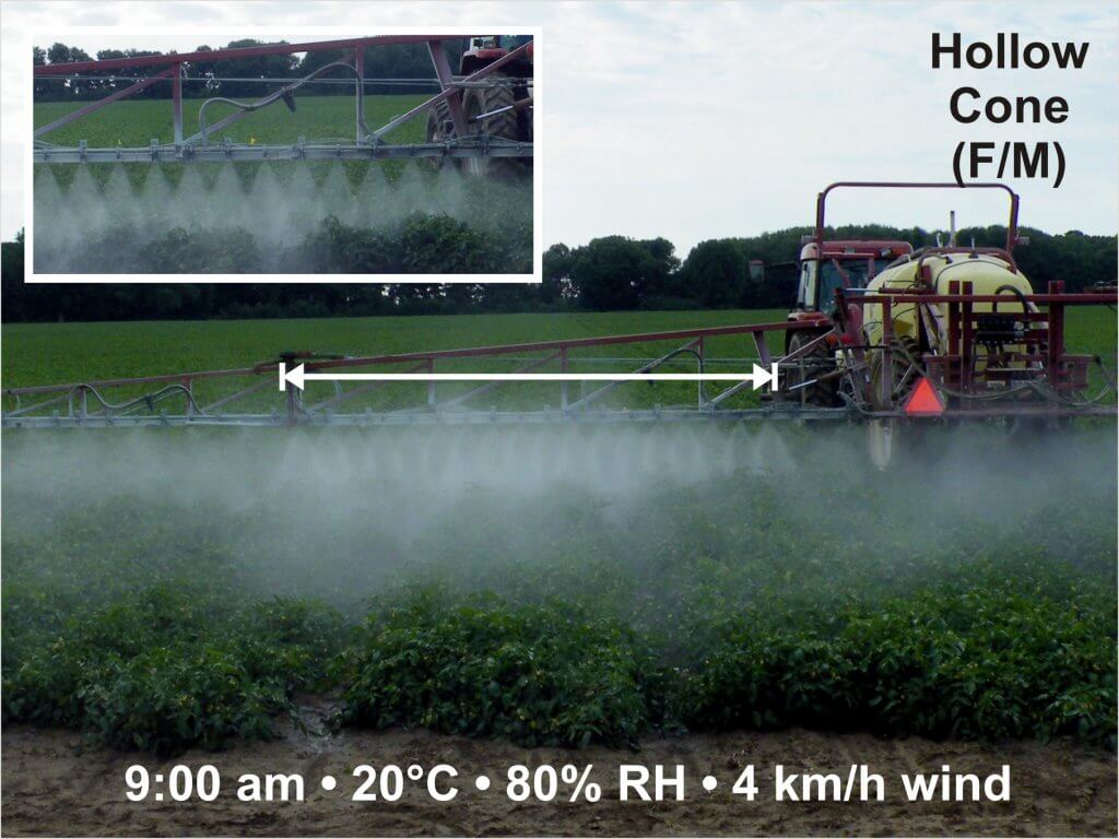
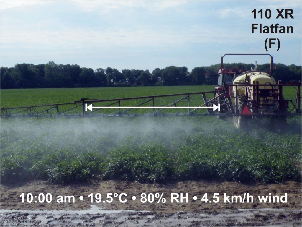
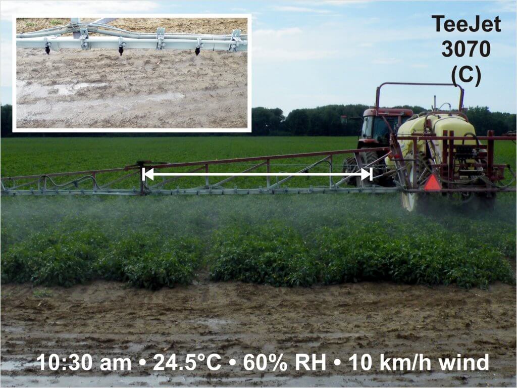
Once again, we used water-sensitive paper. This time we placed two pieces back-to-back (face up and face down) about 1/3 down into the canopy. Then we placed two more in the same orientation about 2/3 down into the canopy. We did this for three plants for each pass. The next four images show the visual drift and weather conditions for each nozzle. Note that only one boom section was nozzled (indicated by a white line) in each condition.

Condition 1 – Turbo TwinJet (Coarse Spray Quality)

Condition 2 – Hollow Cones (10″ centres – Fine/Medium Spray Quality)

Condition 3 – XR 110° FlatFan (Fine Spray Quality)

Condition 4 – TeeJet 3070 (Coarse Spray Quality)

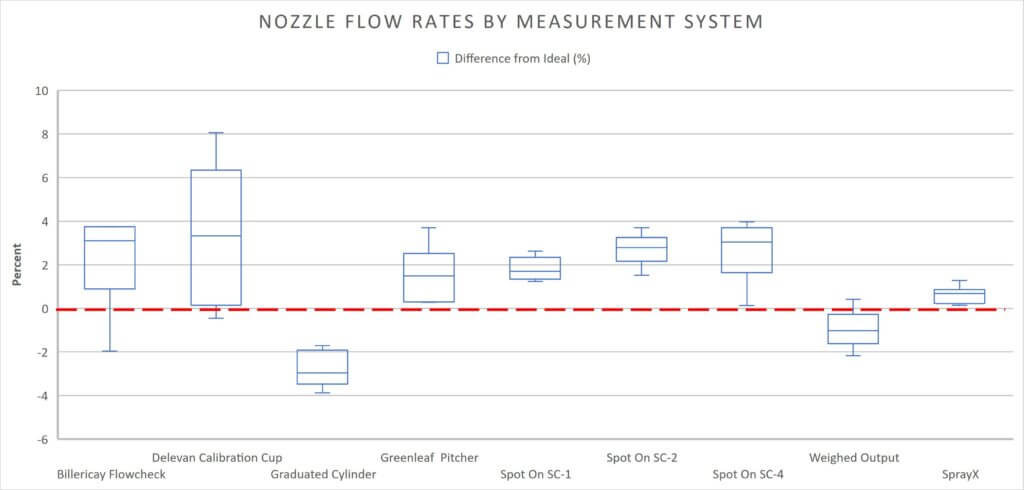
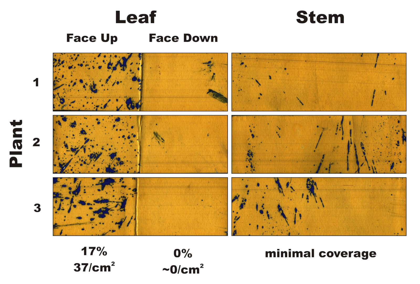
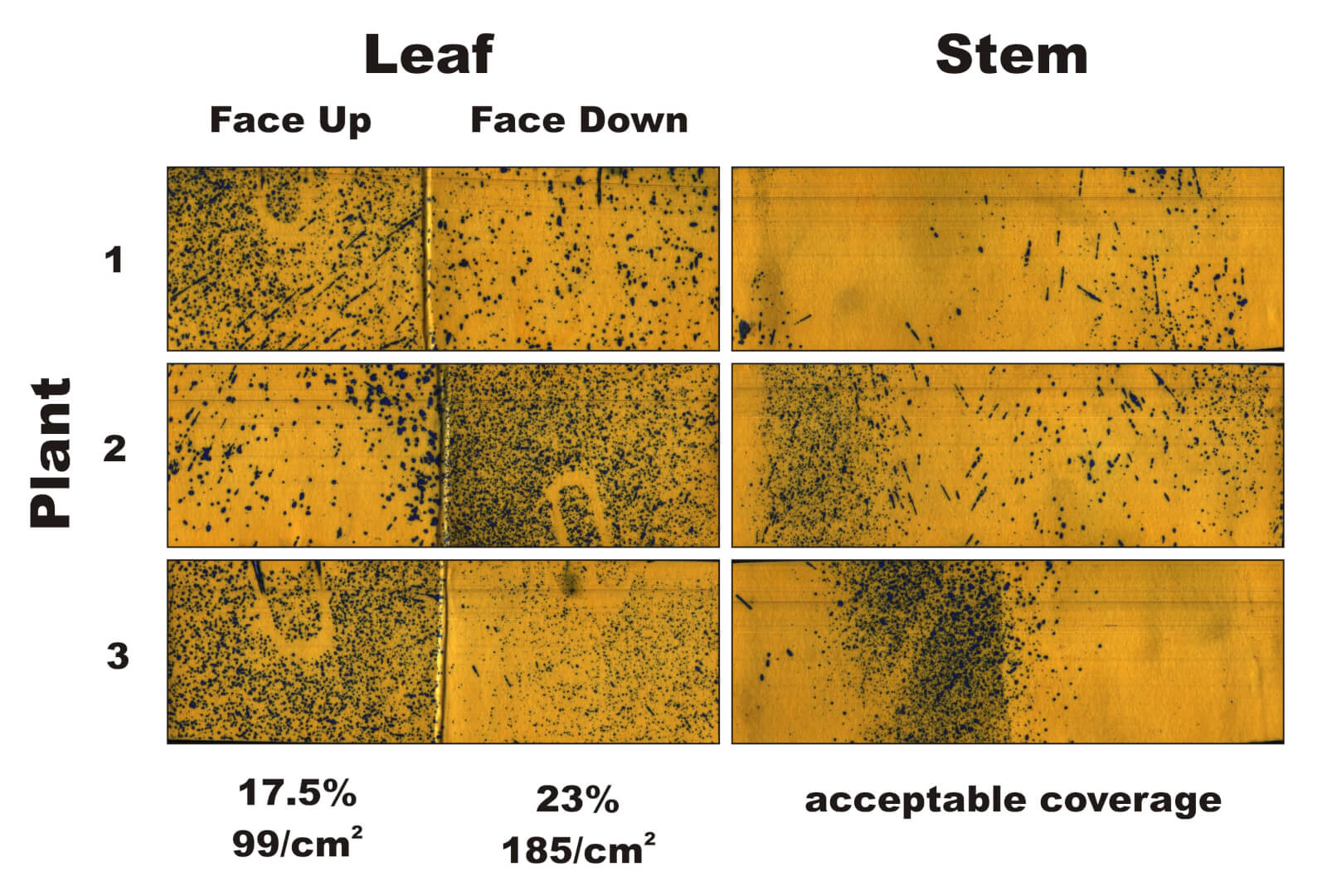
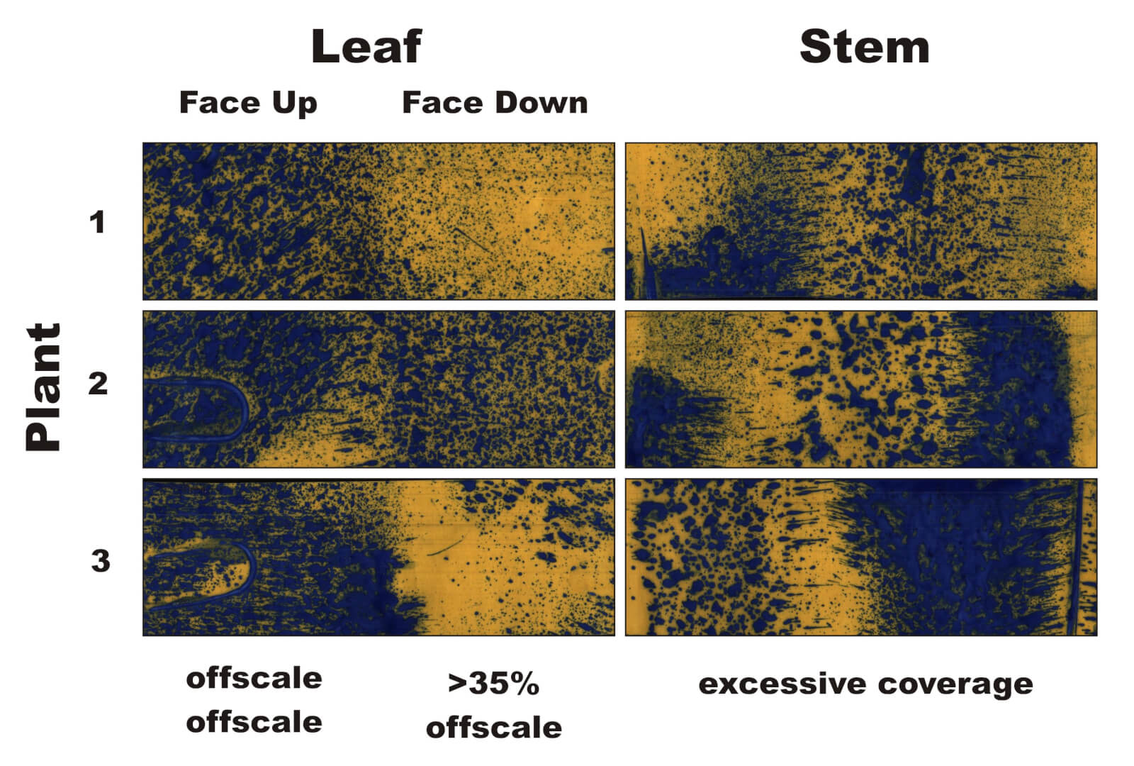
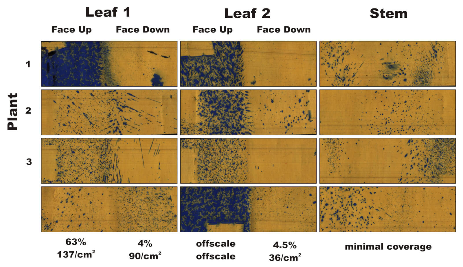
It was very humid, making it difficult to place and retrieve the papers without smearing them. This made it tricky to discern differences in coverage, and the blurring prevented us from quantifying droplet density (i.e. number of drops per unit area). Nevertheless, papers were scanned and the percent coverage was calculated using the DepositScan software developed by the USDA’s Dr. Heping Zhu. The average percent-coverage (± S.E. n=3) is shown in the image below.

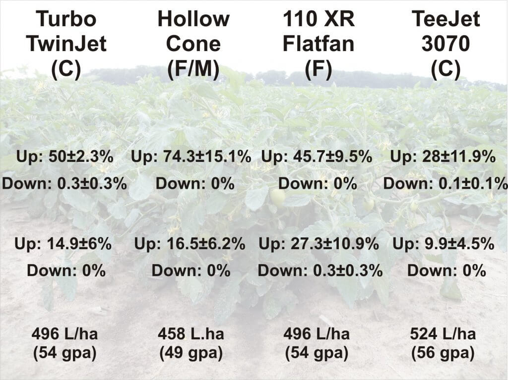
Coverage on the upward-facing papers in the upper portion of the canopy showed excessive coverage for all nozzles but the 3070. Little or no coverage was detected on the downward-facing cards, but without air-assist or a directed application (e.g. drop arms), this was expected. It’s the deeper canopy that’s of particular interest. The only significant difference may lie in the XR flat fan which showed more coverage on the upward facing papers and some (however little) on the downward facing papers.

This came as something of a surprise given that the XR produced a Fine spray quality and there was no air assist to guide spray into the canopy. I believe the high humidity and low winds played a role in this outcome by reducing evaporation and off-target drift. On a drier, windier day, we likely would not have seen this level of inner canopy coverage for either the XR or the hollow cone. By comparison, the Turbo TwinJet with its Coarse spray quality not only reduces off target drift, but would be more resilient in drier and windier weather and may very well have produced the best coverage by comparison.

Take Home

Drawing from both studies:

Properly calibrated air assist will reduce drift and has promise to improve canopy penetration/coverage.
Spray shape (e.g. twin, hollow cone, flat fan) does not seem to play a role in canopy penetration.
Spray quality larger than Coarse may negatively impact canopy penetration in tomato.
Coarse spray quality is perhaps the most versatile option when volume is sufficient (>500 L/ha).
Fine-Medium spray quality is only a viable option in high humidity and light winds. However, air assist is critical to counter drift, and high spray volumes (>500 L/ha) are still required despite the higher droplet count.
Underleaf coverage is exceedingly difficult to achieve, even with finer spray quality and air assist.

This occurred in Ontario (date and location withheld). The sprayer missed the outer edge of the tomato field during a late blight application. An unintentional field check, and amazing to see the results.

August 4, 2022

Methods for Testing Nozzle Flow Rate
Calibration should be a regular practice for every operation that uses a sprayer. Part of that process is confirming that each nozzle is operating within the manufacturer’s specifications. This is a must for researchers that adhere to Good Laboratory Practices and for custom operators that sell their services. But we didn’t just fall off the turnip truck… we know nobody else does it. In fact, we’re surprised when we hear an operator HAS checked their nozzle flow.
And we get it. It can be awkward and time consuming. A field sprayer with 72 nozzle bodies and three nozzles in each position has a whopping 216 nozzles. A tower-style or wrap-around airblast sprayer has fewer nozzles, but the operator needs a ladder to reach them all and they don’t point straight down, so a tube must be used to guide the spray into a collection vessel.
And when pressed, any operator that does not regularly check their nozzles counters by saying “my tank empties in the same place every time, so why check them?” Even if the sprayer does start to go further on a tank, the operator can speed up or adjust the rate controller to drop the pressure a little.
Fair enough. This isn’t a hill we choose to die on.
But we will say that nozzles worn by even a few percent don’t only cause a change in flow rate, but may indicate a deteriorating spray quality and spray geometry. And, when one (or a few) nozzles are worn and others are not, it’s the same as when a single nozzle is plugged – the operator won’t be able to tell from the cab because the rate controller tends to mask the problem. And, if using PWM to apply a simultaneously reduced broadcast rate, perhaps the issue is amplified? All of this impacts coverage uniformity.
We’ll get off our soapbox now.
Over the years we’ve encountered many methods for determining a nozzle’s flow rate. We wanted to try each of them and characterize their accuracy, precision, time required, and ease of use. This is not a ranking where we wanted to find “The Best” method. The best method depends on your situation. If you’re a researcher, then accuracy and precision may trump time and expense. If you’re a custom applicator, then perhaps time is the critical factor. And if it’s your own operation, perhaps expense matters most. It’s up to you.
Method
The following tests were performed on a spray patternator table. A single nozzle was operated by a ShurFlo 2088-594-154 positive displacement pump. Pressure was set using a bypass regulator and an analog pressure gauge, confirmed by a SprayX digital manometer positioned under the nozzle body via a splitter. Room temperature water was used.
“Patty” the spray patternator table. Designed and constructed by Mohawk College, Brantford, Ontario.
Digital manometer on a splitter parallel with the test nozzle.
We tested ten nozzle flow rate measurement systems. There are others out there, but we limited the selection to farmer-oriented systems and not those used in mandatory government inspections.
1. Billericay Flowcheck
2. Delavan Calibration Cup
3. Graduated Cylinder
4. Greenleaf Calibration Pitcher
5. SprayX SprayFlow Turbo
6. SpotOn SC-1
7. SpotOn SC-2
8. SpotOn SC-4
9. Weighed Output
10. Lurmark McKenzie Calibrator
Three samples were taken from a new TeeJet XR8004 at ~40 psi and three samples taken from a new TeeJet AIXR11004 at ~70 psi. An exception was made for the Billericay Flowcheck which specified 43.5 psi (3 bar) for all sampling. All systems were emptied or dried as much as their design permitted between samples.
All data was converted to gallons per minute and the flow measured was compared to the calculated flow for the nozzle and pressure used. For example, if the manometer read 38 psi for the 8004, then the formula 0.4 x (38 psi ÷ 40) ^0.5gives us a calculated flow of 0.39 gpm. If the method reported 0.41 gpm, then it would be off by +5.1%.
Results
Consider the accuracy and the precision of each system when you review the results. Remember that precision means you get the same result with very little variation while accuracy means that on average you get the correct result. And, for context, remember that most recommend changing a nozzle when it is 10% more than the ideal flow rate. We prefer 5%, and if three or more nozzles are off spec, replace them all as a batch because they’re likely all very close. Compared to most spraying costs, a set of nozzles is not worth quibbling about. Some operators just change them annually and don’t bother with testing at all.
Billericay Flowcheck: This is a passive measurement system. You must select the nozzle size on the bottom of the collector and suspend the unit from the nozzle body. It’s designed for a horizontal boom and you’d have trouble using it with any other sprayer. You also have to set the pressure to exactly 43.5 psi (3 bar). While fairly accurate, it spanned about +/-2.5% off ideal. You have to read from the right scale, which in this case was red and rather difficult to read because of the low contrast. It took about two minutes to reach equilibrium for each reading and a lot of liquid is lost during the process.
We attempted to keep the unit plumb so the meniscus and scale aligned correctly. We found it difficult to read the ’04 scale because of low contrast. Pictured is 1.53 lpm.
Delavan Calibration Cup: This small, one-handed plastic cup had a scale printed on the outside. We were limited to a 15 second collection because of how quickly it filled. Some spray was lost to mist and bounce and we used the “Fluid Oz” scale to get the highest resolution from the measurement. It took less than a minute to collect and read from the cup, but had the lowest precision and accuracy.
Graduated Cylinder: There was little or no mist or bounce from escaping spray during collection. Our 1,000 ml graduated cylinder took 30 seconds at 40 psi and 20 seconds at 70 psi to fill making it roughly one minute per reading. A few light taps removed bubbles and once the liquid settled we could read the level. This must be performed on a level surface (in our case we used the digital level app on our iPhone). This was a very precise method, varying by less than 2%, but it wasn’t very accurate. We may have introduced error when reading the meniscus (always read from the centre) or perhaps the plastic distorted over time and affected accuracy. It may be difficult for most people to get a high quality, scientific-grade graduated cylinder.
Greenleaf Calibration Pitcher: The pitcher had multiple scales but once again we used fluid ounces because it had the highest resolution. With the highest capacity, we were able to collect for an entire minute. Despite holding the vessel at different angles and distances, we lost a lot of spray to mist and bounce and the nozzle body was beaded with water at the end of each trial. After tapping the vessel to remove bubbles and reading on a level surface, it took about 1.5 minutes per sample and averaged an average 3% more than the calculated ideal flow rate.
Innoquest Spot On Digital Calibrator: We’ll discuss all three Spot Ons together. The Spot Ons were a game-changer in North America when they first came out. You can read a peer-reviewed article about the SC-1 by Dr. Bob Wolf et al. published in 2015 in the Journal of Pesticide Safety here. The SC-2 is a new version of the SC-1 with added digital features that allow the user to calculate gallons per acre and it indicates tip wear based on the 10% industry standard . The most important improvements were a reduced sensitivity to foam and a thicker foam diffuser to reduce the chance of errors. The SC-4 works exactly like the SC-1, but has a larger capacity intended for high flow rate nozzles (e.g. hollow cones on an airblast sprayer). In each case, the Spot On will report in several units, and must be held steady under the nozzle flow (i.e. not moved during reading). The SC-1 and 2 took less than 12 seconds for each reading and the SC-4 took closer to 30. The SC-1 and SC-2 were relatively precise but read consistently higher than the calculated flow rate. This may be an artefact given that the units only read to 2 decimal places and this may have exaggerated any error. The SC-4 was the least accurate and precise of the three. The Spot Ons were the fastest and easiest to read of the methods used.
Weighed Output: This method is based on the fact that 1 ml of water weighs one gram. Spray was collected for 30 seconds and weighed on a new, $25 CAD digital kitchen scale, which was tared (i.e. the weight of the vessel subtracted from the overall weight). While subject to errors from manual timing, it has the merit of removing the challenge of reading a meniscus and it’s relatively inexpensive. This method was precise and relatively accurate compared to the other methods used. It took about a minute per sample.
SprayX SprayFlow Turbo: This was the most sophisticated method we used. The kit comes with a digital manometer, a flowmeter and a digital scale. It works though a smartphone app (screenshot below). You first have to set up a virtual sprayer, informing the app how many sections and nozzles will be tested. Then you must calibrate the flow sensor by taking three measurements versus a weighed output to eliminate possible variations caused by the nozzle, pressure, temperature, and the density of the liquid. The app walks the user through each step. This method took the most time to set up (easily 10 minutes). However, once it was set up, each nozzle could be tested in less than 30 seconds apiece. This method was the most accurate and precise, but the price may place it out of reach for the typical user.
Screenshot from the SprayX SprayFlow app.
Lurmark McKenzie Calibrator: This method is not reported in the box-and-whisker plot because there were significant problems that prevented accurate readings. It was difficult to get a seal over the nozzle and the floater ball would either stick or fluctuate. After several attempts, this method was abandoned.
Conclusion
In order to test if a process, or a thing, is occurring or produced within acceptable limits, we need a detection system with a high enough resolution. In manufacturing (e.g. factory production) this is an essential requirement in quality assurance. Let’s consider a +10% deviation from the nozzle’s ideal flow rate to be our indication that a nozzle needs to be replaced. We need a measurement system with an appropriate scale and one with sufficient precision to ensure we don’t get a false reading. Based on our data, I would suggest all systems reviewed, save the measurement cup, are viable. Even if we elect to use a more stringent rejection threshold of 5%, some systems are more precise than others (i.e. less variability), but all but the cup should still be sufficient.
What’s the penalty for not testing, assuming we’re not talking about significantly deviant nozzles? Let’s say, for example, we are not using a rate controller and we are applying 20 US gpa at 12 mph using 72 nozzles on 20″ centres. Our boom would have to spray 58.2 gpm, which means each nozzle would have to emit 0.81 gpm. If those nozzles sprayed 5% more than intended, we’d be spraying 21 gpa instead of 20 gpa. That means for a 1,200 gallon sprayer, you’d do 57 acres instead of 60. We would have the same result if we dropped from 12 mph to 11.45 mph, which is about 5% slower. Maybe that’s a big deal for your operation, or maybe not. For most, 5% is well within the typical error inherent to spraying. Then again, perhaps it’s more important to know that each nozzle is performing in a manner similar to its neighbours to ensure the highest degree of coverage uniformity.
Ultimately, it is important to ensure you’re as efficient as possible, and that means understanding what your nozzles are doing so you can decide if-and-when it’s time to replace them. Pick whichever method makes it easiest for you to justify testing your nozzles and do it at least once a year when you take your sprayer out of long term storage.
Thanks to all the companies that donated or loaned their calibrators to make this article possible.
July 5, 2022
Herbicides in Asparagus – A creative solution
In 2016, an asparagus grower in southern Ontario picked up a used De Cloet Hi-Boy originally used to spray tobacco. His vision was to create a three-row herbicide sprayer for asparagus and we were invited to participate. His concept was to design shrouds that would contain the herbicide, but not snag the asparagus or drag heavily on the ground. This article follows the development of the sprayer from concept to testing to final product.
The sprayer itself was a classic three-wheel, self-propelled affair. The asparagus was planted on four foot centres, leaving a three foot alley. While the goal was to hang three shrouds off the boom, we started with one to work out the bugs.
This operation uses 2,4-D to control weeds in the alleys and while a little can hit the asparagus stem up to 12 inches (where the branching starts), we wanted to avoid contact at all costs. That led us to the TeeJet AI 95° flat fan nozzle, which produces a Very Coarse to Extremely Coarse spray quality. A single nozzle could be suspended to span the 3 foot width of the alley.
The first version of the shroud was suspended off the boom from four anchorage points. A certain amount of of play was allowed so the shroud would find plumb (i.e. hang vertically), even when the sprayer boom yawed or pitched over uneven ground.
The shroud was constructed of sheet metal, angled to reduce the potential for contact with the asparagus branches, and terminated in stiff, nylon brush-style mud flaps commonly seen on trucks. These brushes were cut to a few inches in length to span the distance between the side of the shroud and the ground. This would create a “seal” to prevent spray from escaping, maintaining some degree of contact with uneven ground.
We tested the first version by placing water sensitive paper in two positions on the ground, just inside the reach of the brushes. We had to be careful not to run them over with the centre wheel of the sprayer. We also adhered two papers to the angled inner walls to see how much, if any, spray was hitting the inside of the shroud.
Our first pass on June 16th was at 9:00 am, 19.1 ºC (66.4 ºF) with a cross wind of 5 to 7 km/h (3.1 – 4.3 mph). relative humidity was high at 85% and travel speed was slow at 3.2 km/h (2 mph). We started with the .06 AI tip at 50 psi, but we drenched all the targets with excessive coverage because we were travelling so slow. We also found the stiff brushes were creating furrows in the soil, as shown below.
For our second pass, we tried the .04 tip and raised the shroud while dropping the tip to keep it suspended 15 inches over the ground. We were still drenching the targets and noticed the shroud was hitting the asparagus spears, causing physical damage. The damage is shown below – note the dark green on the bent spear.
This led to a decision to flare the side walls more aggressively, bringing them further into the centre of the alley and away from the spears (shown later in the article). This had the added benefit of angling the brushes as well to get a maximum span for weed control in the alley. For the final coverage pass we used the AI .03 tip, which gave more than 45% coverage on the ground, with even distribution, and there was no indication of spray on the papers adhered to the inside of the shroud. This coverage is more than is likely required, and the operator should be able to spray up to 6.5 km/h (4 mph) without compromising coverage.
Since the coverage tests, the grower added additional sheet metal fenders to the the existing fenders, encasing the wheels and creating a smooth transition for the shroud to gently deflect the asparagus. The fenders were needed because the grower found the asparagus was being pushed out by the wheel fender only to bounce back in front of the shroud, which snagged the fern and damaged it. The additional fenders keep the fern spread and prevent it getting caught in front of the shrouds.
The grower was very happy with the sprayer’s performance and planed to build another. Why be satisfied with the status quo when you can tap into your creative side and be innovative? If you don’t think you’re imaginative enough to try upgrading equipment on your farm, here’s a simple test to prove that it’s in you. It’s easy to see the bird in the image below, but with a little concentration you’ll be rewarded with a ski-jumping rabbit.
Thanks to TeeJet for donating the nozzles and water-sensitive paper and to Ray and Brad Vogel of Lingwood Farms for inviting me to participate.
Learn more about spraying asparagus here.
June 6, 2022
Gear up – Throttle down
In 1977, David Shelton and Kenneth Von Bargen (University of Nebraska) published an article called “10-1977 CC279 Gear Up – Throttle Down”. It described the merits of reducing tractor rpm’s for trailed implements that didn’t need 540 rpm to operate. In 2001 (republished in 2009), Robert Grisso (Extension Engineer with Virginia Cooperative Extension) described the same fuel-saving practice. Again, it was noted that many PTO-driven farm implements don’t need full tractor power, so why waste the fuel? He tested shifting to a higher tractor gear and slowing engine speed to maintain the desired ground speed. 700 diesel tractors were tested, and as long as the equipment could operate at a lower PTO speed and the tractor itself didn’t lug (i.e. overload), as much as 40% of the diesel was saved.
How this applies to Airblast
For airblast operators with PTO-driven sprayers and positive-displacement pumps, this has potential for reducing air energy. Gearing up and throttling down (GUTD) sees the operator reducing the PTO speed from 540 rpm to somewhere between 350-375 rpms, which not only saves fuel but more importantly slows the fan speed. This may be an option when air energy from the sprayer, even at higher travel speeds and a low fan gear, still overblows the target canopy.
Some airblast sprayers, like this one, feature fan blades with manually-adjustable pitch to increase or lower air volume and speed. It’s often a pain to try to adjust them, and most operators only try it once.
A good time to try this out is early in the spraying season when (most) canopies are dormant and at their most sparse. For example, when applying dormant sprays in apple orchards, look to see if the wood on the sprayer-side gets wet, but does not creep around the sides. This suggests that the air, and much of it’s droplet payload, are being deflected. When the air speed is slowed, it will become more diffuse and turbulent on target surfaces, and this turbulence helps more droplets deposit in a panoramic fashion within (not past) the target canopy. Look to see if the wood is wet >50% around the circumference of the branches. You’ll get the rest when you spray form the other side.
Limitations
GUTD is not always appropriate. It requires airblast sprayers with PTO-driven positive displacement pumps (e.g. diaphragm). Airblast sprayers with centrifugal pumps would experience a drop in operating pressure and would have to be re-nozzled. Further, the pump must have sufficient surplus capacity to maintain pressure at low rpms.
GUTD is not intended for air-shear sprayers that employ twin-fluid nozzles because dropping air speed below a certain threshold may compromise spray quality; the air needs to be fast enough to create and direct spray droplets
The tractor must have sufficient horsepower (more than 25% in excess of minimally-required capacity) to permit the reduction in engine torque. This is especially important if the operator is on hilly terrain. If the tractor begins to lug (e.g. black smoke, sluggish response, strange sounds) you’ll be in trouble.
Observations
We first experimented with GUTD in 2013. We noticed how much quieter the sprayer was, and the fuel consumption was certainly reduced. One grower-cooperator switched to a GUTD spray strategy mid-way through their dormant oil application in pears. We saw the trees immediately began to drip. Panoramic coverage was improved significantly; once the operator passed down the other side of the target, capillary action and surface tension helped to give near-complete coverage.
However, in one instance, the operator was already applying a low spray volume per hectare using air induction nozzles and their lowest fan gear. By further slowing fan speed using GUTD, coverage at the top of his cherry trees was compromised.
In short, GUTD can work under the right circumstances. If you want to try it, use water-sensitive paper to establish a base-line with your current practice, and then evaluate coverage after you change your sprayer settings.
May 18, 2022
Drop Hoses Improve Coverage in Field Peppers
In early July 2016, a farm supplier contacted us on behalf of a client with a history of disease control issues in his field pepper operation. He wanted us to calibrate their sprayer and diagnose spray coverage to see if there was room for improvement. Improved coverage doesn’t necessarily mean improved efficacy, but generally it’s a reliable indicator. When we arrived at the field the winds were gusting over 15 km/h, which had the potential to create a massive drift issue. We were only spraying water, so it was decided that if we managed decent coverage in those conditions, there would be no need to worry on an acceptable spray day.
Field pepper in Southern Ontario in mid-July
The grower traditionally ran two different settings on his sprayer. They were relatively low volumes for a vegetable operation, but the crop was still small at this stage, so we did not propose raising the volume:
1. TeeJet AITX 11008’s on 50 cm (20″) centres at 11.25 kmh (7 mph) and 3.44 bar (50 psi). That’s 3.35 L/min (0.89 gpm) per nozzle for a total rate of 350 L/ha (37.5 gpa).
2. TeeJet ConeJet TXVK18’s on 50 cm (20″) centres at 7 kmh (4.5 mph) and 3.44 bar (80 psi). That’s 1.6 L/min (0.42 gpm) per nozzle for a total rate of 275 L/ha (29.5 gpa).
To test the coverage with these settings, we folded a piece of water-sensitive paper over a leaf to cover both surfaces, and wrapped one around a hollow tube to mimic a plant stem (see figure). Three plants were papered for each sprayer pass. Papers were collected, digitized and analysed for percent-coverage and droplet density. When diagnosing coverage for a horticultural crop, a distribution of 85 medium deposits/cm² and 10-15% coverage is a reasonable standard for most applications.
Location of water-sensitive papers in situ.
The first condition (the AITX tips) averaged 17% coverage on upper leaf surfaces (37 deposits/cm²). These were coarser droplets at relatively low volume, so it was no surprise that we didn’t achieve 85 deposit/cm² target. When using such large droplets, it is more important to achieve an even distribution and the 10-15% surface coverage (we achieved 17%). There were no deposits on the underside of the leaves (See figure 1), but that was also expected as coarser droplets tend to follow a downward vector that is not conductive to under-leaf coverage.
Figure 1 – Water-sensitive papers from three plants sprayed in Condition 1. Percent coverage and droplet density are calculated for the leaves, and a visual inspection is made of the stems.
The second condition (the ConeJets) provided better coverage. The fine droplets produced covered an average 17.5% coverage with a distribution of 99 deposits/cm² on upper surfaces, and 23% coverage with a distribution of 185 deposits/cm² on lower surfaces. Panoramic stem coverage was improved as well (see figure 2). This is excellent coverage, but the finer droplets were highly prone to drift (see below). With no form of drift control, this set up is undesirable.
Figure 2 – Water-sensitive papers from three plants sprayed in Condition 2. Percent coverage and droplet density are calculated for the leaves, and a visual inspection is made of the stems.
With no form of drift control, the finer droplets produced by hollow cones create unacceptable spray drift, even in moderate wind conditions.
This led us to propose a more directed boom arrangement: We set up a hollow cone over the row (the grower’s original ConeJet) and a drop hose suspended in each alley with two TeeJet XR 8004 flat fans positioned on an angle (i.e. not vertical or horizontal to ground). This gave sufficient height to span the canopy with as little direct waste on the ground as possible. As the crop grows, the nozzles would need to be twisted into a more vertical alignment.
ConeJet TXVK18’s alternating with drop hoses with TeeJet XR 8004’s.
We did not use an air induction fan to avoid the Very Coarse spray quality and we used 80° instead of 110° to ensure the spray did not overshoot or undershoot the plant. Here are the details of the third set up:
3. TeeJet ConeJet TXVK-18’s on 100 cm (40″) centres at 7 kmh (4.5 mph) and 3.44 bar (80 psi). That’s 1.6 L/min (0.42 gpm) per nozzle. Also, two TeeJet XR 8004’s per drop on 100 cm (40″) centres at 7 kmh (4.5 mph) and 3.44 bar (80 psi). That’s ~4.5 L/min (1.2 gpm) per drop hose. Together, set of nozzle for a total rate of 523 L/ha (56 gpa).
This set up raised the volume considerably and aimed spray directly at the sides of the plant. Coverage was excessive and in a few cases exceeded what the diagnostic software could reliably resolve (see figure 3). Since the plants were still small at this stage, it was decided we would let them “grow into the volume” and come back to check coverage once they were at full size.
Figure 3 – Water-sensitive papers from three plants sprayed in Condition 3. Percent coverage and droplet density are calculated for the leaves, and a visual inspection is made of the stems.
When we returned in mid-August the plants had reached full maturity. In this final coverage trial, we added a second water-sensitive paper to each plant to span the height of the crop canopy, which had grown considerably.
The same pepper plants ~5 weeks later had more than doubled in size.
Coverage was reduced compared to how we left things in July, but appeared to be sufficient on key surfaces (see figure 4). The papers showed upper leaf-surface coverage of 63%-to-offscale and deposit distribution of 137 deposits/cm²-to-offscale. Coverage on the lower leaf surfaces was greatly reduced to 4-4.5% and 36-90 deposits/cm². Panoramic stem coverage was present, but minimal. Applying higher volumes would likely have improved matters.
Figure 4 – Water-sensitive papers from three plants sprayed in Condition 3, ~5 weeks later. Percent coverage and deposit density are calculated for the leaves, and a visual inspection is made of the stems.
When asked about the drop hoses, the grower reported “They are a bit of a nuisance because they take extra time to put on, and they get caught in the bush at the back of the field. But if they increase our coverage, then they’re worth the extra effort.”
Final thoughts
Adding drop hoses to a vegetable sprayer may be unconventional, but if fungicide coverage is a concern, and the drops will fit between rows, they might be worth a try. Carefully consider the volumes you use because they should reflect the size of the plant canopy you are trying to protect. Finally, water-sensitive paper provides excellent feedback to help you decide if your field volume, nozzle rates and nozzle positions are providing acceptable coverage.
April 22, 2022