The decision on which application method is best for herbicides boils down to two main factors: (a) target type and (b) mode of action. In general, it’s easier for sprays to stick to broadleaf plants on account of their comparatively larger leaf size and better wettability compared to grassy plants. There are exceptions, of course – at the cotyledon stage, broadleaf plants can be very small and a finer spray with tighter droplet spacing may be needed. Water sensitive paper is a very useful tool to make that assessment. Imagine if a tiny cotyledon could fit between deposits – that could be a miss!
Some weeds are also more difficult to wet, and those may also need a finer spray or a better surfactant for proper leaf contact. An easy test is to apply plain water to the leaf with a spray bottle. If the water beads off or the droplets remain perched on top in discrete spheres, the surface is considered hard to wet. Most grassy weeds are hard to wet, while most broadleaf weeds are easy to wet.
Grassy weeds are an especially difficult target because they have smaller, more vertically oriented leaves, and almost without exception are more difficult to wet than broadleaf species. All these factors call for finer sprays for effective targeting and spray retention.
Broadleaf weeds usually have more horizontally oriented leaves which also happen to be larger. As a result, they can intercept larger droplets quite efficiently.
There are about thirty mode of action (MOA) groups among the herbicides with about ten accounting for the majority in Canadian prairie agriculture. It’s probably an over-simplification to categorize them into just two groups – systemic and contact. But that grouping goes a long way to making an application decision.
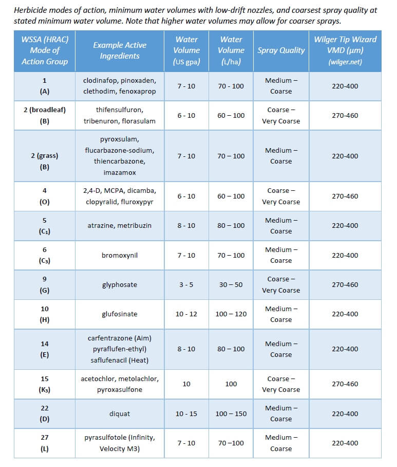
Contact products (MOA Group 5, 6, 10, 14, 22, 27) must form a deposit that provides good coverage. Good coverage is an ambiguous term that basically means that droplets need to be closely spaced and cover a significant proportion of the surface area because their physiological effects occur under the droplet, and don’t spread far from there. One way to generate more droplets is to reduce droplet diameter, another is to add more water. A reasonable combination of both is ideal because simply making droplets smaller creates issues with evaporation and drift.
Systemic products (MOA Group 1, 2, 4, 9) will translocate within the plant to their site of action after uptake. As a result, coverage is less important as long as sufficient dose is presented to the plant. In practice, this means coarser sprays and/or less water may be acceptable.
When two factors are combined, either in a tank mix or a weed spectrum, the more limiting factor rules. Application of a tank mix or product that is active on both broadleaf and grass plants will be governed by the limitation placed on grass targets. A tank mix comprised of both systemic and contact products is governed by the limitations placed on contact products.
A factor we should also consider is soil activity and the presence of residue. Studies have shown that soil-active products are relatively insensitive to droplet size. But if they have to travel through a layer of trash to get to the soil surface, more application volume is the best tool.
Below are some recommended spray qualities and water volumes for use in Canada. The spray qualities listed in the table can be matched to a specific nozzle by referring to nozzle manufacturer catalogues, websites, or apps. Note that Wilger also offers traditional VMD measurements on their site, allowing users to be a bit more specific if necessary.
If you read this site, you know we’re fans of recirculating booms. We love them for three reasons:
They save money and waste by recovering spray back to the tank during priming and rinsing
They make boom cleaning easier by eliminating boom-ends
Most require individual nozzle shutoff, which makes for better sectional control
If you’re new to the concept of recirculating booms, read more here.
Until recently, these booms were only available on sprayers imported from outside North America (Horsch, Amazone, Agrifac to mention three), or via France’s Pommier booms that have been available as retrofits for many years. In 2018, Agco introduced their Liquid Logic system on the Rogator line, becoming the first North American manufacturer to offer a recirculating boom at the factory. Pattison Liquid also offers Recirculating booms as standard equipment on their Connect Sniper pull-type sprayer.
In the meantime, three boom retrofit kits and one sectional conversion kit have become available.
Arag Australia‘s BRS (Boom Recirculation System)
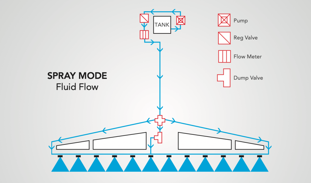
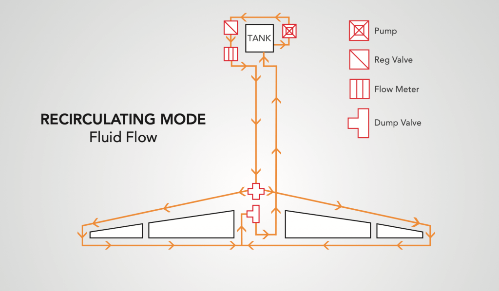
The first was developed by Arag Australia, and is available there via Nozzles Online, and in Canada through Nozzle Ninja. Designed for John Deere R-Series and Case Patriot sprayers, the kit uses the existing line that feeds liquid to the outermost section and simply extend that line to the end where it enters the boom via two installed elbows. The liquid returns to the centre via the installed boom sections which are connected together by removing the boom end cap (or “aspirator” for John Deere) and replacing the gap with a section of hose. Back at the centre rack, the liquid from both booms meet in the middle. At this point, a three-way valve gives the choice to return the spray to the tank, or to receive pressure from the pump. There is also a manual valve that allows the return to be dumped for safe disposal.
Arag Boom Recirculation System (Spray Mode)Arag Boom Recirculation System (Recirculation Mode)
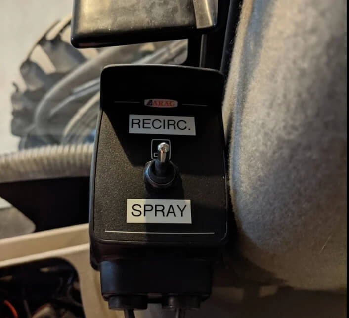
The system does not tie into the sprayer’s electronics. instead, it adds a switch in the cab that the operator uses to switch from spray mode to recirculation mode. The switch is not activated at the end of each swath, but instead to prime or flush the boom.
A switch is added so the user chooses recirculation or spray mode. The boom would recirculate to prime or flush, and remain in spray mode during the spray operation.
Raven
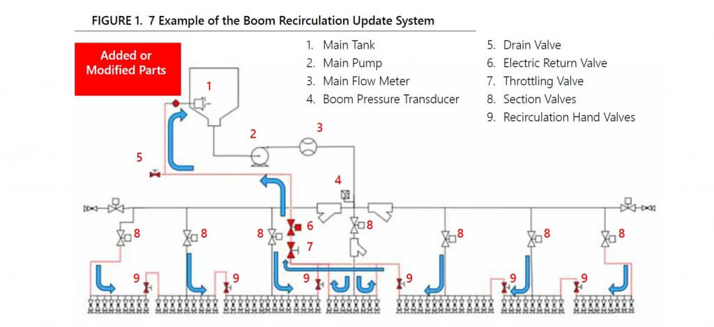
Raven offers a recirculation kit for 3000, 4000, and 5000 series Case Patriot sprayers with Aim Command HD and an ISOBUS terminal. The approach is slightly different, as they retain the pressure feed through individual sections but also tie the sections together so the spray is returned to the tank. By including a shutoff valve between each section, the system retains the option to use conventional sectional control for high flow situations, or to isolate a section should a leak occur. The system can be configured and controlled from the sprayer monitor, either a Viper 4+, CR7, or CR12.
Raven Boom Recircualtion System schematic (from Raven manual). Note the retention of section valves and the addition of manual valves between sections.
John Deere
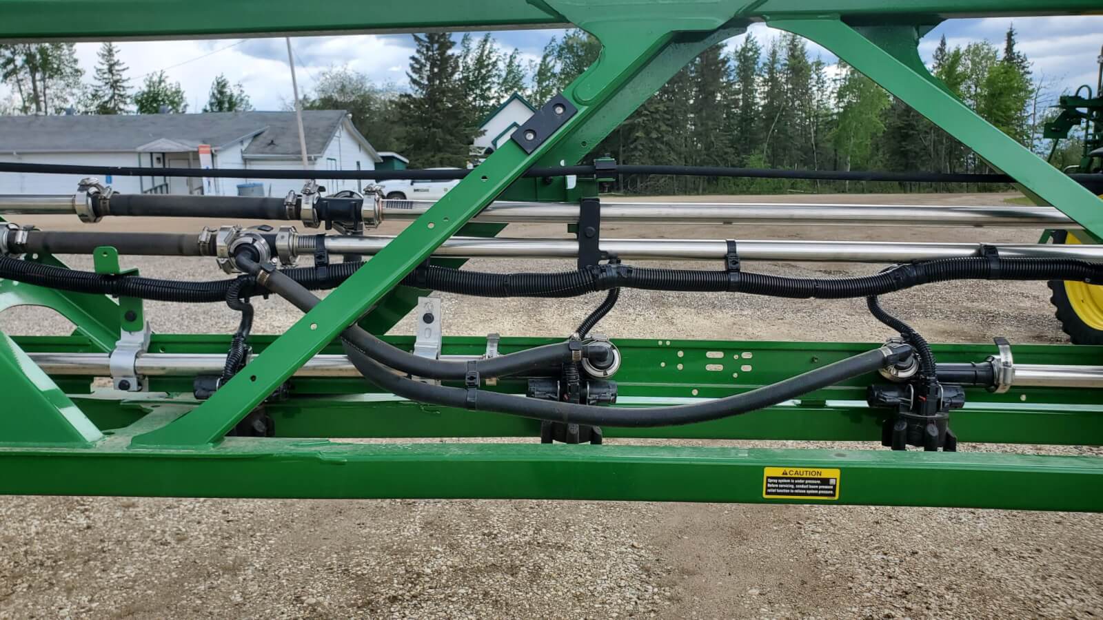
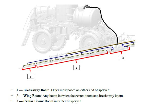
On March 2, 2021, John Deere announced a 2022 factory option called Pressure Recirculation and Product Reclaim. The system keeps several existing sections and adds two steel lines the flull length of each boom wing. One is for supply, the other return. As these lines approach a section, the supply is fed to one end of the section and the return is connected to the other end. On a 120′ boom, there are five recirculating sections, two on each wing and the centre.
This approach adds one more line than the other designs, and this line will hold materials that ultimately need to be cleaned, flushed, and possibly dumped or sprayed out for cleanout. A possible reason for the extra line is the ability to deliver 220 gpm to the boom, an advertised feature of John Deere high flow booms that may come in handy for topdressing liquid fertilizer. These levels of volume are not needed for pesticides.
John Deere Boom Recirculation and Reclaim. Top two lines are supply and return and extend the length of each boom wing. These connect to the existing sections on each wing, creating several smaller recirculating sections.
Latitude Ag
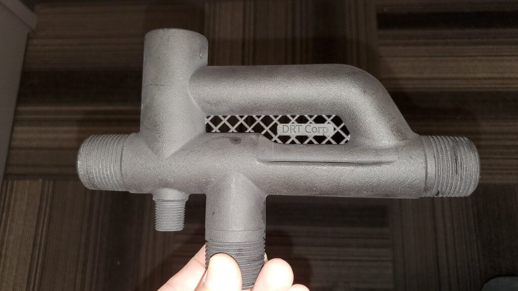
This Wisconsin company has developed an innovative product that converts any existing plumbed section that contains boom ends into a recirculating section. It does this by incorporating a boom recirculation valve” (the “Merlin IC System“) into the original section feed line. Boom end caps are removed and replaced with sweeps and hoses that return flow to these boom valves. The flow from the boom ends is incorporated back into the sectional feed thanks to a venturi design in the recirculation valve.
A prototype of the Merlin IC System valve made by Latitude Ag
Advantages of this design include simplicity. No moving parts are required, the valve simply recirculates the flow from the boom ends automatically whenever that section operates. Existing sectional control, whether it’s by plumbed section or individual nozzle bodies, is unaffected. Flushing the boom with water is done with normal spraying. It takes some extra time to incorporate and dilute the contents of the boom end return lines but results in a clean boom and no section end residue. We’ve seen the results of testing and agree that it works.
This product does not allow boom priming without spraying. However, a key advantage is that it can be used with direct injection since no product is returned to the tank. Latitude Ag says it will provide the necessary flow sensor and software to make this possible. As of 2025, this system may no longer be commercially available.
Precision Planting ReClaim
ReClaim is capable of operating on a sprayer with or without individual nozzle shutoff. For conventional nozzle bodies containing the original spring-loaded diaphragm check valves, the concept is to drop the liquid pressure below the cracking point of the check valves so flow continues through the sections and back to the tank without engaging the nozzles.
Recirculation fittings are added to the end of each boom section. These feed into 3/4″ lines are installed on section ends, which in turn feed increasing diameter collector lines that eventually return all flow to the tank. Flow reaches the sections as before. When recirculation is turned on, flow exits the boom section through the new fittings and returns through 3/4″ lines to the centre of each section, where it enters 1” lines that take the flow to the center of each boom wing. There the flow in the 1” lines is combined moves to the center of the sprayer on 1.5” lines where it meets the flow from the other wing. From there, the flow returns to the tank through an electronic ball valve and 2” line. This system ensures no back-pressure and balanced flow from each section.
For some sprayer rate control systems such as John Deere, the pump won’t operate below about 20 psi despite operator settings. This means the priming or flushing procedure would trigger nozzles to spray if the bodies were fitted with spring-loaded diaphragm check valves. A pressure reduction kit (a second restrictor valve) is required to reduce the pressure sufficiently for ReClaim to work in these instances. More here.
ReClaim operates independently of any electronic control systems, relying on a toggle switch to initiate recirculation. When flow back to the tank is detected, a light indicates that recirculation is working, and the operator waits approximately 60 sections for a 120’ boom to circulate all volume back to the tank. Download the operator’s guide, here.
This system requires a lot of additional lines. A 120’ boom would require 120’ of additional 1” line and 60’ of 1.5” line. The manufacturer states that ReClaim adds about 14 gallons of volume that would need to be displaced back to the tank, adding to the standing volume. This volume can be circulated using solution from the main solution tank, or displaced back to the tank using flow from an existing clean water tank, or displaced using compressed air via an optional pneumatic port. It is not clear how spray mix in the ReClaim system can be removed from lines without returning it to the tank and draining it from there. Users should consider the additional surface area and volume that will have to be addressed during cleanout.
Do It Yourself
If none of the available options work for your sprayer, consider building your own system. Sprayer plumbing parts are available from the major manufacturers Banjo, Hypro, TeeJet, and Wilger. Wilger, in particular, has developed a nice suite of parts well suited to recirculating booms, including flanged sweeps and thin gauge steel booms, punched for nozzle bodies or unpunched to move product. See their support for DIY projects on this dedicated page: Wilger Retrofit.
Take Home
All these recirculation options improve the status quo of plumbed boom sections with boom ends. They should be considered essential equipment on sprayers.
This work was performed with Mike Cowbrough, OMAFA Field Crop Weed Specialist.
In the early summer months, many field and specialty crop operations collect rainwater (or possibly pump water from holding ponds) into storage tanks for use as a carrier in spray applications. These tanks may be stationary, or they may be part of a nurse or tender truck that delivers both water and chemistry to the field as a means of improving operational efficiency.
In the case of translucent poly tanks, which are commonly used because of their light weight, custom shape, and low price point, light exposure will grow algae. Algal populations multiply exponentially and will clog spray filters and negatively affect filling. In response, growers use home-grown algicides such as copper sulfate, lengths of copper pipe, household bleach, chlorine, bromine, etc. They do so with little or no guidance and therefore little or no consistency. Beyond the obvious questions surrounding efficacy, it is unknown whether these adjuncts create physical or chemical incompatibilities in the tank mix. If so, there is the potential for reduced efficacy and/or crop damage.
We tested popular methods for algae control by inoculating a series of 10 L translucent plastic jugs with an algal population sourced from a southern Ontario holding pond. The population was left to acclimate and generally establish itself (aka colonize) before we introduced some form of control. Each jug was then gently stirred and emptied through a sieve for qualitative assessment.
In a parallel experiment, we introduced the same algicides to fill water and conducted spray trials. 10 L volumes were mixed with a field rate of glyphosate and sprayed on RR soybeans. Weed control was assessed and soybean yield measured for each treatment.
Algicide Efficacy Experiment
In each treatment, tap water was mixed with a micronutrient growth media (from the Canadian Phycological Culture Centre at the University of Waterloo). This was an unsterilized 10% WC(ed) solution intended to provide micronutrients for algal growth while minimizing fungal and bacterial growth.
The source algae were collected from the bottom of a holding pond from a farm in Guelph, Ontario. Algae were homogenized and equal parts added to each jug. The jugs were former 10 L pesticide containers thoroughly rinsed and sprayed with Five Star’s “Star San” non-rinse sterilizer. Tank solutions were gently bubbled (one bubble every 10-15 seconds) with air from an aquarium pump. Air was balanced using a manifold and introduced via diffusion stones at the bottom of each jug.
Algae sourced from a farm’s holding pond near Guelph, Ontario. Algae was homogenized before inoculating treatment jugs with equal parts.
Treatments
Each treatment was tap water plus growth media inoculated with algae and exposed to a natural diurnal/nocturnal cycle unless otherwise indicated.
Container was spray-painted black to exclude light
Ammonia
“Scotch Bright” copper-coated scour pad. (copper is often introduced as copper sulfate at 1 cup / 1,000 US gal. or a short length of copper pipe)
Bromine (sourced from a local pool supply store)
Treatment Number
Treatment Name
Rate (/US Gal.)
Rate (% v/v)
Rate (/10 L final volume)
1
Control (no algicide)
2
Shaded
3
*Household bleach
1/4 tsp
0.00033
3.3 mL
4
Black container
5
*Ammonia solution
1/4 tsp
0.00033
3.3 mL
6
Copper-coated scour pad
7
Bromine
1/32 ml
0.000004
0.04 g
Table 1. *Bleach and ammonia should never be added together as they produce toxic chloramine gas.
Method
On July 12, jugs were loaded with water and growth media and inoculated with algae. They were bubbled gently for one week to establish a stable algal colony. On July 19, algicides were added, or transferred to shade or black-out conditions. On August 31 (approximately six weeks later), jug contents were gently stirred and filtered through white cloth for qualitative assessment.
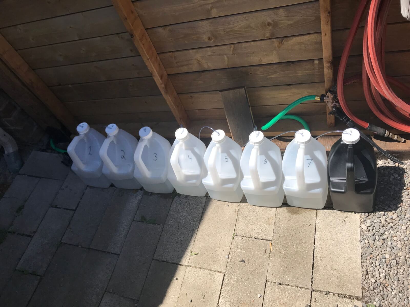
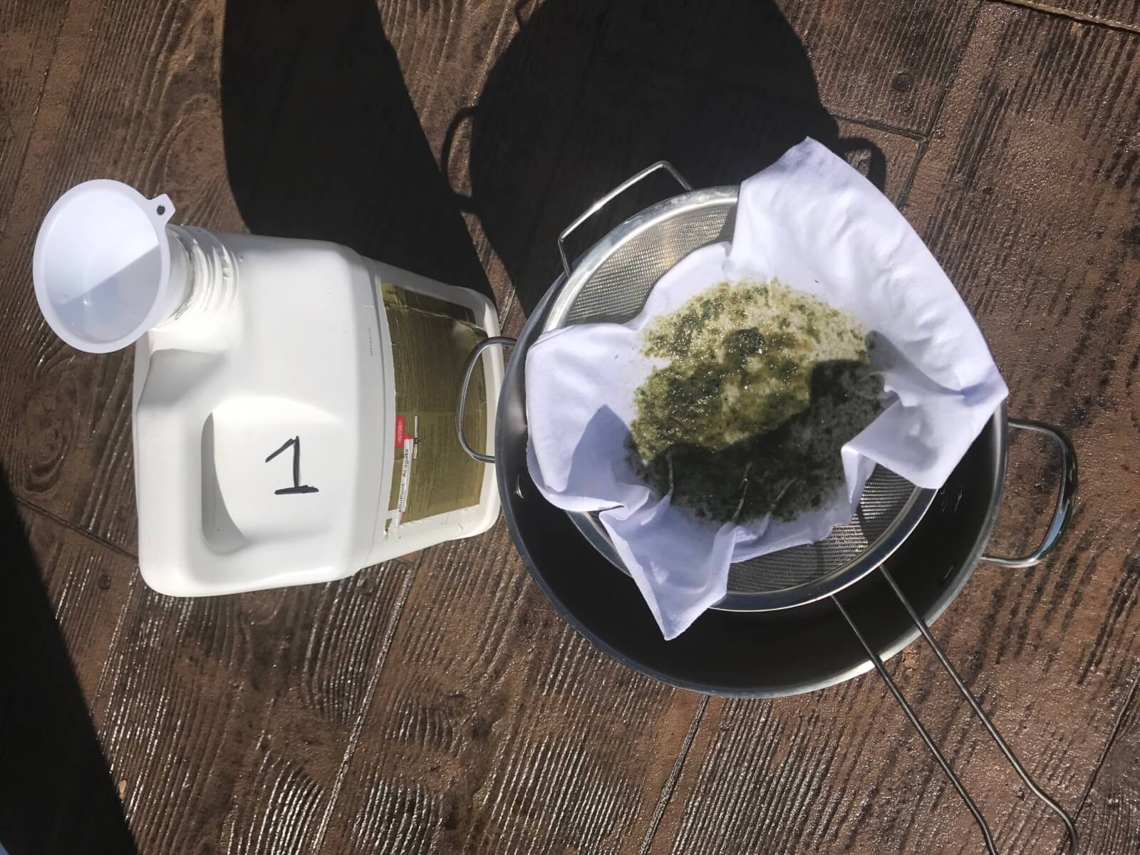
Building up algal population for each jug. Note air lines through lids for slow, intermittent bubbling. Algae was not moved to black container or to the shade until after the first week of acclimation.Almost six weeks after algicide was added, jug contents were gently stirred and poured through white cloth to collect algae and establish how easily the liquid passed through.
Observations
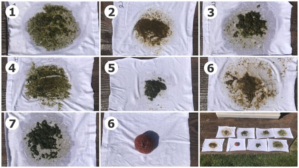
The results of all seven treatments, plus photos of the copper-coated scour pad.
(1) Control. Liquid poured slowly through cloth. Algae was still alive and healthy. It formed some clumps but was not as thick as other treatments.
(2) Shaded. Liquid poured fast and easily through cloth. Was particulate in texture rather than clumpy or gelatinous. Very little mass and entirely brown, suggesting it was dead.
(3) Household bleach. Liquid poured easily through cloth until the clump of algae sitting at the bottom of the jug came out (i.e., most algae were not suspended). Thick mat of healthy-looking algae (note profile photo #3 below). Much greener and thicker than the control (1).
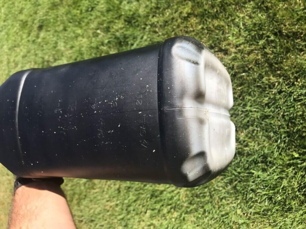
(4) Black container. Liquid poured fast and easily through cloth. Algae retained a little green coloration (more than the shaded condition (2)) but was particulate and not as healthy as the control (1). We intended for this treatment to exclude all light, but it was still able to enter at the bottom where the jug wasn’t completely painted. This may have kept the algae alive.
In an oversight, the jug was not completely painted. This left a source of light at the bottom edge that may have helped sustain algae.
(5) Ammonia. Very difficult to pour liquid through the cloth (note profile photo #5 below). The only condition where a mat of algae was floating at the top of the jug rather than settled at the bottom. It was healthy, green and thick.
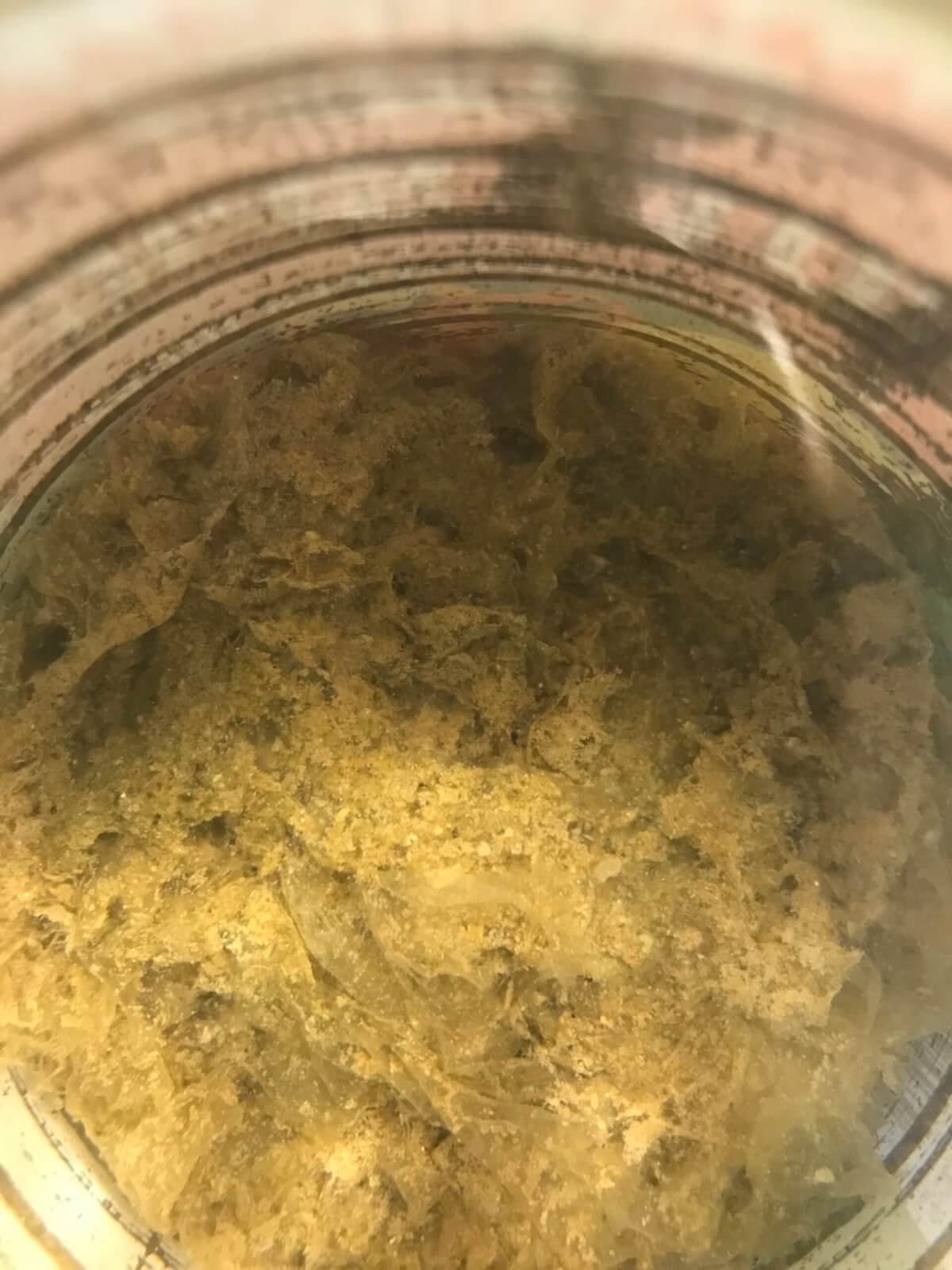
(6) Copper. The most gelatinous of all conditions, the liquid took the longest to pass through the cloth filter. While the algae seemed brown and dead, the gel would be very problematic during sprayer filling and spraying. Note that the copper scouring pad (shown unrinsed) has nothing growing on it.
(7) Bromine. Like the household bleach condition, liquid poured easily until the healthy mat of algae at the bottom of the jug came out (i.e., most algae were not suspended). Note profile photo #7 below.
Profile shots of treatment 3 (Bleach), 5 (Ammonia), and 7 (Bromine).
Spray Efficacy Experiment
Ideally, adjuncts added to carrier water are inert. That means they don’t reduce a herbicide’s effectiveness on susceptible weeds or increase crop injury. For example, hypochlorite (found in bleach and in chlorinated water) reduces the biological effectiveness of low concentrations of isoxaflutole (the active ingredient in herbicides such as Converge and Corvus). However, when added to higher, agriculturally-relevant concentrations, the reduction in efficacy wasn’t considered significant (Lin et al., 2003). Conversely, bromide has been added to certain herbicides to improve performance (Jeschke, 2009).
There’s precious little information about synergistic or antagonistic effects from adding bleach, ammonia, copper or bromine to herbicide carrier water. To learn more, we added each of these adjuncts to the standard rate of glyphosate (900 gae/ha – 0.67 L/ac). Using a CO2-pressurized plot sprayer, the solution was applied to <10 cm tall weeds at 150 L/ha (15 g/ac) in glyphosate tolerant soybean at the 2nd trifoliate stage of growth (Elora Research Station, Ontario).
Visual crop injury was evaluated at 7 and 14 days after application. Weed efficacy was evaluated at 14 and 28 days after application. Soybeans yields were collected using a Wintersteiger plot combine and adjusted to a moisture content of 14%.
Weed Control
All treatments provided excellent control (>90%) of the weeds emerged at the time of application. Table 2 (below) presents the % visual control 28 days after application.
Carrier Treatment (glyphosate 540 g/L at 900 gae/ha or 0.67 L/ac)
Lamb’s-quarter
Green pigweed
Witch grass
Green foxtail
1) Control
0
0
0
0
2) Shaded
100
100
100
100
3) Household bleach
100
100
100
100
3a) Household bleach – added prior to mixing
95
97
100
100
4) Black container
100
100
100
100
5) Ammonia
100
100
100
100
6) Copper-coated scour pad
100
100
100
100
7) Bromine
100
100
100
100
Table 2. Visual control of lamb’s-quarter, green pigweed, witch grass and green pigweed at 28 days after the application of glyphosate 540 g/L at 900 gae/ha mixed with various carrier treatments intended to prevent algae growth. Treatment numbers correspond with the soybean injury and yield image below.
Soybean Injury and Yield
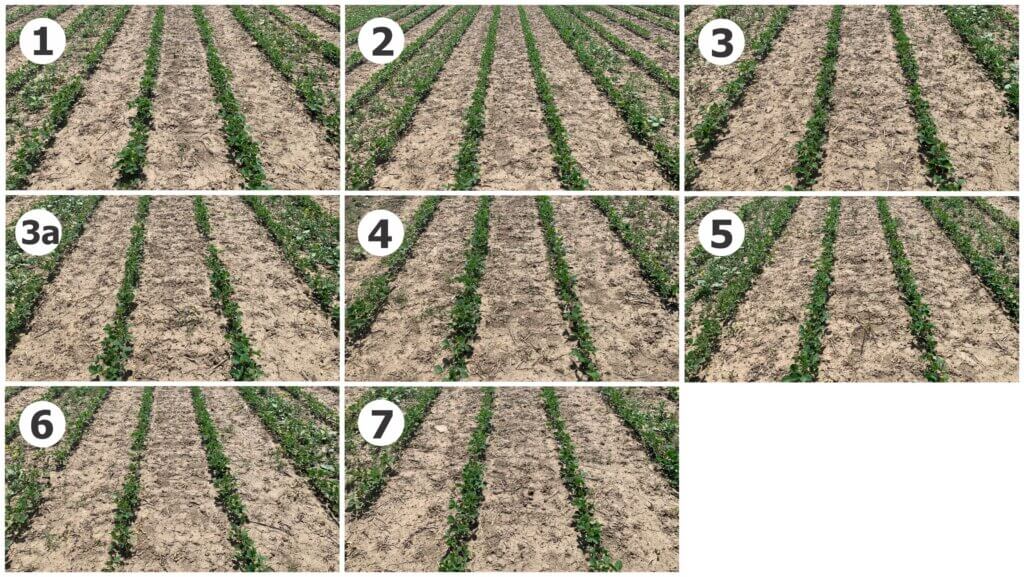
There was no noticeable crop injury from any treatment (figure below) and yields were not significantly different from the control treatment (Table 3). However, when bleach was added prior to mixing, we did observe a trend in reduced soybean yield. We’re unable to explain this observation, but suggest it may be an unrelated issue (such as field variability). There were no obvious signs of crop injury, and the treatment provided excellent weed control.
Photographs of each plot 14 days after application. The number/letter in each inset image corresponds to treatments in Tables 2 and 3.
Carrier Treatment (glyphosate 540 g/L at 900 gae/ha or 0.67 L/ac)
Crop Injury (%)*
Avg. Yield (bu/ac)
Significance**
4) Black container
0
40.0
A
7) Bromine
0
39.6
A
2) Shaded
0
38.1
AB
3) Household bleach
0
37.6
AB
1) Control
0
37
ABC
5) Ammonia
0
36.9
ABC
6) Copper-coated scour pad
0
36.1
BC
3a) Household bleach – added prior to mixing
0
34.0
C
Table 3. Visual control of lamb’s-quarter, green pigweed, witch grass and green pigweed at 28 days after the application of glyphosate 540 g/L at 900 gae/ha mixed with various carrier treatments to prevent algae growth. *7 days after application. **Duncan’s multiple range test. Soybean yields that don’t share a letter in common are significantly different.
Discussion
We elected to use an extreme situation where a single application of algicide was applied to an established, healthy colony. It’s possible that regular applications of algicide in a volume of water with little or no algae could maintain that condition.
A treatment was considered effective if it slowed or halted algal growth, especially if it also degraded algal populations, causing them to become brown, thin, and/or particulate. Once in the spray tank, the shear forces created by circulation should disperse any dead or degraded algal masses, making it easier to pass them through filters and nozzles.
The shade treatment appeared to kill algae as well as cause degradation. Second place went to the black-out treatment, where some light was unfortunately allowed in. This would have continued to fuel photosynthesis in the unpainted portion at the bottom of the jug. Conversely, the black exterior likely raised temperatures above >20 °C, which depresses most algal growth and may have contributed to the degradation.
Copper appeared to kill the algae but also created a gel that would pose problems to filters. Unlikely to be bacterial, as copper is known to suppress bacterial growth, it could have been caused by diatoms; certain invasive species are known to form brown jelly-like material endearingly referred to as “brown snot” or “rock snot”. Alternately, and according to work by J. Rodrigues and R. Lagoa, alginate polysaccharide can form viscous aqueous dispersions (such as gels) in the presence of divalent cations (such as copper).
No treatment appeared to reduce herbicide efficacy or affect crop health. However, unexpectedly, the household bleach added prior to mixing may have reduced soybean yield. Given the limited number of replications and the single plot location, we suspect this was a field effect, unrelated to the treatment.
Take Home
Based on these results, a combination of shade and light-excluding materials (e.g. black paint) would be the ideal approach to algae control. It’s cheap, effective, and doesn’t require periodic management. Buying black tanks is a good choice, or you can paint them. What you should paint them with is a matter of debate and there’s a very good Twitter thread on the subject if you’re interested.
An Aside: Algae in Ponds and Dugouts
We didn’t test this, but the question has come up and the best we can do is share some long-standing farmer wisdom. Some have used Aquashade dye to absorb the photosynthetic wavelengths and reduce algae buildup. Reputedly it is moderately successful. Another option is adding aluminum sulfate to the pond, and with a lot of agitation it should clarify in about 48 hours. Still others have added a few square barley straw bales to the water and found it to work surprisingly well (possibly an allelopathic response). Tie a rope to them and float them in the pond.
Citations
Jeschke, Peter. 2009. The unique role of halogen substituents in the design of modern agrochemicals. Pest Manag Sci, 2010; 66: 10–27
Lin, C.H., Lerch, R.N., Garrett, H.E. and M.F. George. 2003. Degradation of Isoxaflutole (Balance) Herbicide by Hypochlorite in Tap Water. J. Agric. Food Chem. 2003, 51, 8011-8014
An “Alternate Row Middle (ARM)” traffic pattern is where the sprayer passes down every second row. The intent is to improve work rate by cutting the driving time in half. The operator hopes to provide suitable coverage on both the sprayer-facing half of the canopy, and that half of the canopy facing the next alley. In our experience, this depends on sprayer design, and only works in very small/young plantings (or only for the first few applications of the season). Even then, the side facing the sprayer tends to get saturated in an effort to ensure a threshold dose reaches the far side. We’ve already captured the pros and cons of ARM in this article, and (spoiler alert) unless you’re using a wrap-around style design, it’s generally not the best approach for protecting an orchard, bush, cane or vine crop.
So why on Earth would we be testing it here?
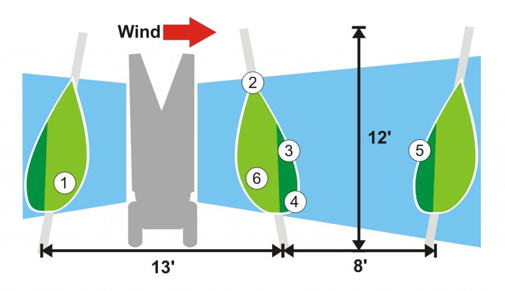
We were contacted by an orchardist who planted a test block of Gala (est. spring, 2017) in an unusual way. He called it “V-Trellis Vertical Axis Cross”. Basically, he created an orchard architecture that only allowed equipment (e.g. platforms, sprayers) to pass down every second row. He figured it would save 35% of his labour costs. In the photo and illustration below, you can see the posts lean over the drivable alleys, creating a “V” shape.
So, given that he couldn’t fit a sprayer down every row, we had no choice but to try to optimize sprayer settings for ARM applications. Note the six numbers in circles in the above illustration. They indicate where we would eventually place water-sensitive papers to diagnose spray coverage.
Here are the settings the orchardist was using before we made any adjustments:
Turbomist sprayer with 11 foot high tower
Bottom-most nozzle was on and every second nozzle position skipped for a total of 5 nozzles active per side
Nozzles were TeeJet ceramic disc-core. Top to bottom: D3-DC45, D3-DC45, D3-DC45, D3-DC45, D3-DC25
7 km/h (4.35 mph) travel speed per a speedometer app on a smartphone
Tractor engine speed was 2,150 rpm (PTO was ~ 540 rpm)
Fan set in low gear
Pressure was 190 psi
Ambient wind gusting to 8 km/h, temperature of 30°C, RH ~65%.
And here is a video of what the sprayer was doing before we changed any settings. This is a single upwind pass, and as you can see, the spray blew through at least five downwind rows. Obviously, this was far too much air and spray volume.
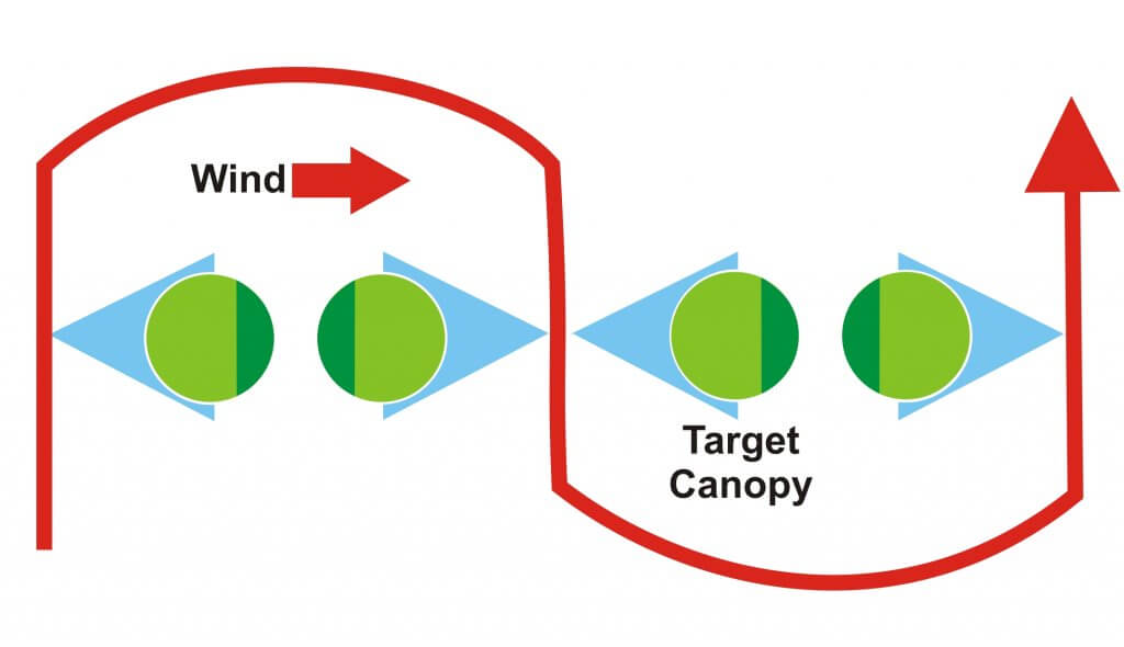
When we diagnose coverage in an every-row situation, we drive the alleys on each side of the target row (i.e. two passes). But, when diagnosing ARM spraying, we want to account for every drop of cumulative coverage from spraying upwind rows. So, we have to do three passes, as shown in the illustration below. In this top-down diagram, the sprayer travels the red line.
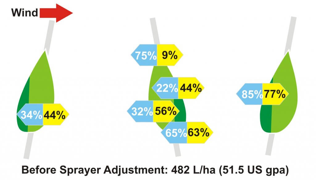
In order to establish a baseline, we diagnosed coverage for the original settings using water-sensitive papers in the six positions indicated above. We folded them in half, so a sensitive side faced each alley. We sprayed water and later digitized the cards to determine the percent coverage on the papers. Remember, if 80% of the cards receive at least 10-15% surface coverage and a deposit density of 85 drops per cm2, it’s typically sufficient.
Here are our results, with percent area-covered indicated in each position, as well as a representative scan of one of the papers. There’s no need to provide deposit density, which after about 30% surface coverage cannot be reliably determined.
So, if the video doesn’t convince, then the papers certainly do: This was way too much air and spray mix.
Next, we performed a series of air adjustments using ribbons (detailed here and here) which led us to reduce engine speed from 2,150 rpm to 1,300 using the Gear-Up, Throttle-Down method. Then we used the OrchardMax calculator to establish an ideal spray volume and guide us to which nozzle rates we should use:
Bottom-most nozzle was on and every second nozzle position skipped for a total of 5 nozzles active per side
Top nozzle was TeeJet AITX8002, followed by TeeJet TXR80015, TXR80036, TXR80015, TXR80015
7 km/h (4.35 mph) travel speed per a speedometer app on a smartphone
Tractor engine speed was 1,300 rpm (PTO was ~ 300 rpm)
Fan set in low gear
Pressure was 100 psi
Ambient wind gusting to 4 km/h, temperature of 26.5°C, RH ~70%.
The following video shows the coverage from a single pass (to be clear, no extra upwind pass). We eventually did three passes to capture the cumulative coverage, just like with the first sprayer settings. This video simply serves to show how in ARM applications, the sprayer-facing side always looks much better than the side facing away. Also note how much quieter the sprayer is, as well as the reduced blow-through.
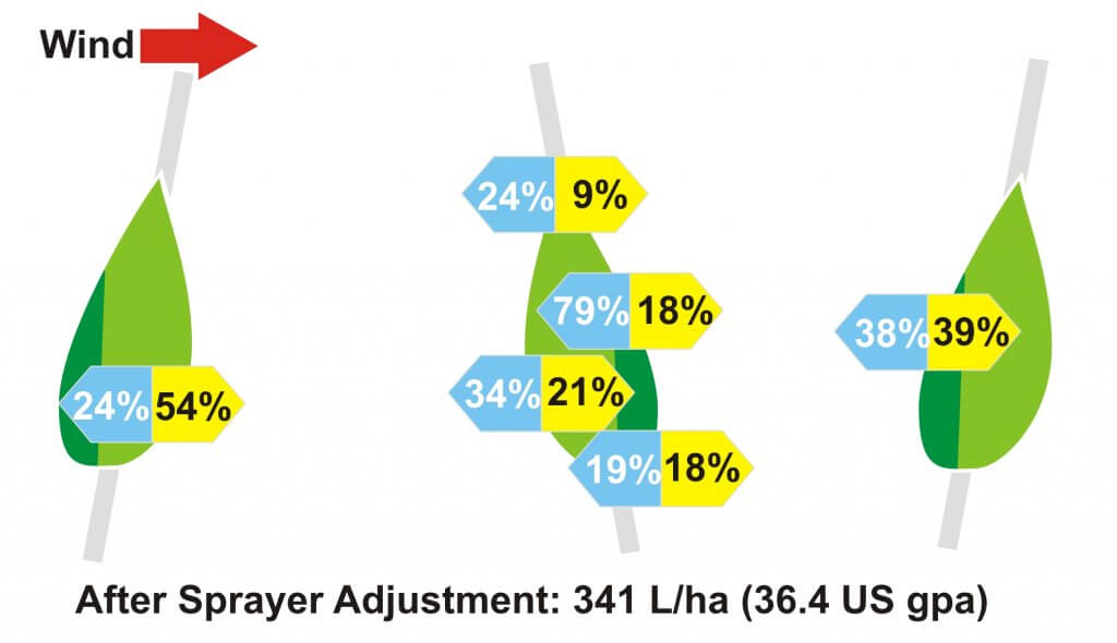
And here is the resultant, cumulative coverage from three passes. Once again, deposit density isn’t required as it exceeded our threshold in each position.
In the end analysis, we saved the grower ~30% of their spray mix, greatly reduced noise and spray drift, and still achieved suitable coverage in the target canopy. So, does this mean ARM applications are redeemed? We refer you, kind reader, to our introduction where we said ARM can work in young plantings and early season applications.
Note that the upwind side of the canopy received less coverage than the downwind side. As this new planting grows and fills, it’s going to be increasingly difficult to achieve sufficient coverage. Changes to the sprayer settings may be able to account for the imbalance, but they will also make the applications less efficient (i.e. more spray mix, more drift and coverage will still not be uniform). It remains to be seen if the spray inefficiency inherent to this orchard architecture is worth the estimated 35% savings in labour costs.
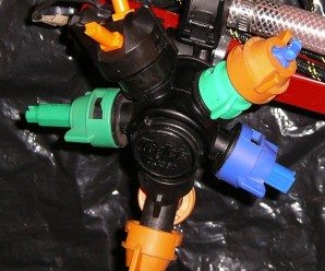
When operators winterize their sprayers, they should remove all the tips and store them separately. Many store them in large pails with lids. Calibrating the sprayer just prior to winterizing will indicate if the nozzles should be stored, or replaced. Let’s assume each tip flow rate is within 5% of the average output and no more than 5% more than the manufacturer’s pressure tables. Yes, industry standard is 10%, but I always wonder how the spray quality suffers with that much wear. Nozzles are, comparatively, a cheap replacement and it’s not worth skimping. Learn more how to check nozzle flow rate, here.
Just like any other part of the sprayer that comes in contact with spray liquid, nozzles (and strainers) should be cleaned regularly. And, just like any other part of the plumbing, the best way to do that is to dilute any residues via a series of rinses. For a more rigorous cleaning, one of the intermediate rinses should include a detergent, and soaking during this step is an excellent practice.
The orifice of any nozzle is delicate, either machined or molded to exacting standards. Even small changes to the orifice shape results in distorted spray (e.g. spray comes out at undesirable angles), a change to the rate (typically more volume per minute) and a change in the spray quality (typically larger median droplet size). If foreign objects or residues remain in the tips, the subsequent spray job may be less accurate and even damage the tips.
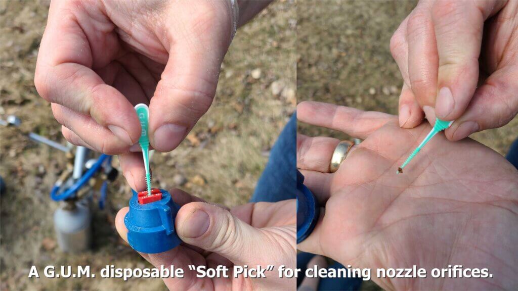
In the case of air induction nozzles, which are essentially the standard on most boom sprayers, debris and weed seeds can plug the air-intake ports. When that happens, the nozzle will not function as intended. So, while the occasional soaking of nozzles does a great deal of good, they may also have to be scrubbed. Don’t use picks or reamers! There are nozzle cleaning tools out there, but they’re basically toothbrushes so save your old ones (and mark them clearly). Soft bristles are the way to go for removing stubborn residues and cleaning any tip orifices, but we found a nifty new way:
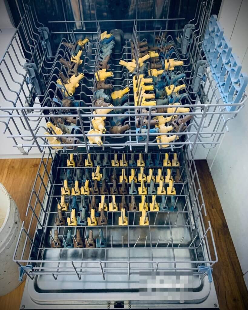
Occasionally we receive photos like the one below and we’re asked what we think. Well, just the same way we don’t recommend cleaning your sprayer overalls in the family clothes washer, we also don’t recommend the use of dishwashers for nozzles.
Not a great idea. Certainly not if you intend to ever use this dishwasher for anything else. And where does the rinsate go?
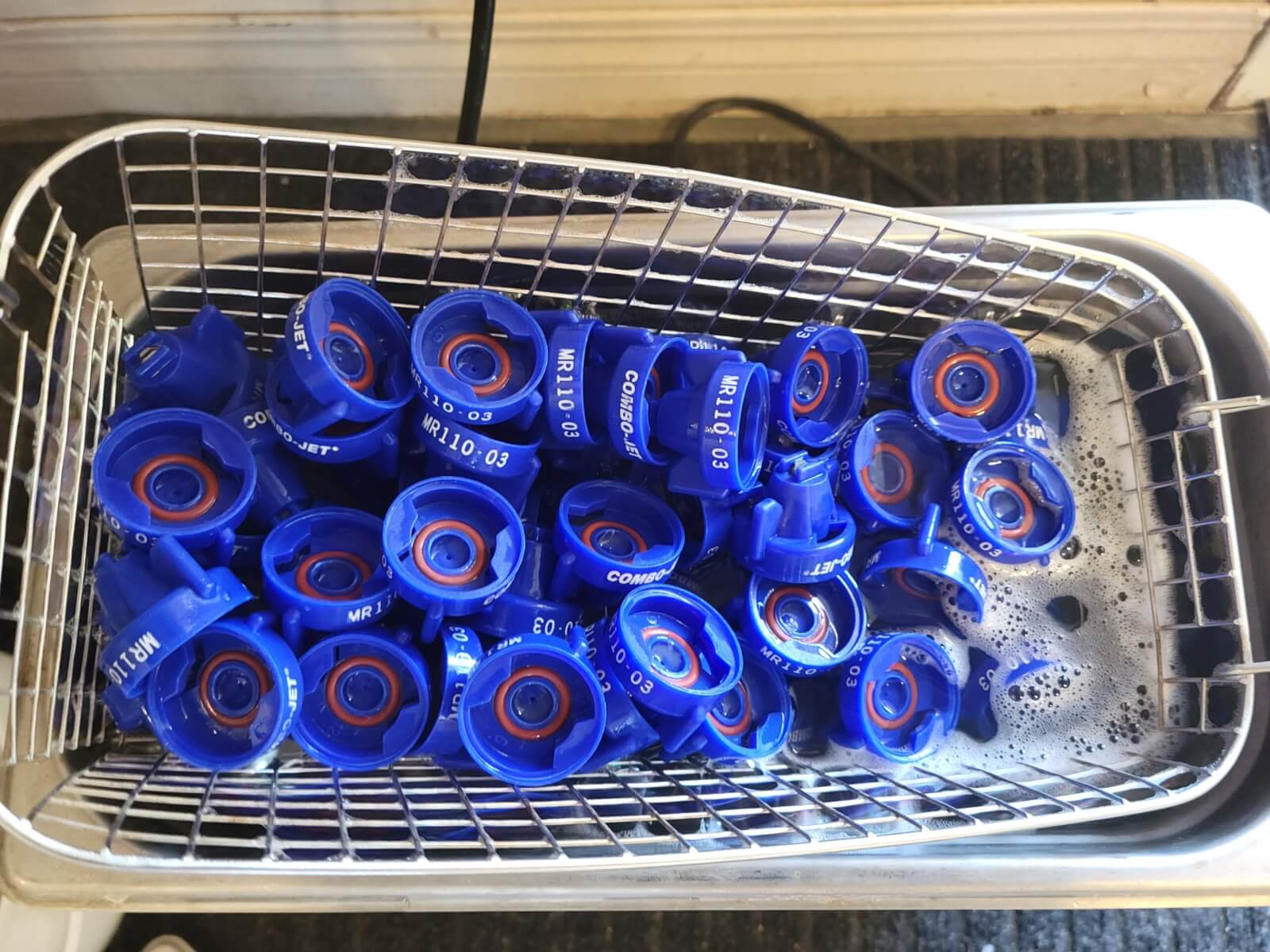
In an interesting experiment, Lucas Olenick of Wilger tried cleaning tips in a heated ultrasonic cleaner. We haven’t tested this and we don’t know what heat and vibration might do to poly and ceramic components, but surely it’s no more aggressive than hot, soapy water and a bristle brush. Lucas tried several durations with and without detergent and arrived at this recipe:
“For tough, non-water-soluble pesticides, around 8+ hours in a heated ultra-sonic cleaner with (Dawn) dish soap to come out like brand new. Other solvents may speed this up, but I’d generally suggest against heating solvents at any concentration. For water-soluble pesticides, expect to be within the 3-6+ hours for the first time to be confident enough in not having to flow-test each of the nozzles. With any pesticides, ensure proper care in handling contaminated nozzles and rinsate after cleaning nozzles.”
The mad genius of Lucas Olenick (@WilgerParts) who used dish detergent and a heated sonic cleaner to unplug tips. Be sure to dispose of rinsate safely. Photo credit: Lucas Olenick.
Don’t have a heated sonic cleaner? No problem. Here’s a step by step:
Wearing gloves, remove all nozzles, strainers, rubber gaskets and tips from the sprayer.
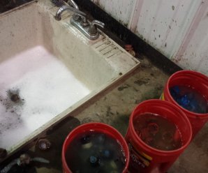
Put them in a large plastic pail and cover them in warm water. Leave them to soak.
Drain the pail, but be aware that the rinsate will have pesticide residue.
Fill a second pail with a solution of the same commercial detergent used to clean the sprayer.
With a toothbrush, scrub the caps, gaskets, strainers and nozzles to remove any residue. Some nozzles can be pulled apart to expose the mixing chamber and facilitate cleaning.
Once scrubbed, leave all the parts to soak in the detergent solution.
Drain the solution, which will contain trace amounts of pesticide, rinse the parts with water and reassemble the nozzles.
While you’re at it, drop those filters and scrub them alongside the tips. This may seem extreme, but of all the technology on a sprayer, the nozzle has the biggest impact on the effectiveness and efficiency of the spray job. Take the opportunity over the winter months to clean and inspect the tips for damage so the sprayer is ready for calibration in the spring.
Soak, scrub, rinse and store nozzles and nozzle strainers. You may replace them once the sprayer is clean, but I prefer to store then separately. Photo credit: Jason Boersma (@RVFBoys), Ridge Valley Farms, Ontario.
Thanks to Jason Boersma (@RVFBoys), Ridge Valley Farms, Ontario, who sparked this article with his tweet: “Great job for a cold winter day, soak & clean all your tips to be ready for spring also saves on down time!”