Category: Spray Basics

  • Calibration – “The Fundamental Relationship”

    Calibration – “The Fundamental Relationship”

    The Fundamental Relationship, a concept by Professor D. Ken Giles (Emeritus), UC Davis Biological and Agricultural Engineering Department, is a way of talking about calibration without numbers and formulas. It is valuable for teaching concepts important to calibration. Since it is a relationship, it describes the variables needed and how they relate to each other.

    The Fundamental Relationship:

    Application Rate (gallons/acre) = Flow rate (gallons/minute) ÷ Land rate (acres/minute)

    We see here that land rate is inversely proportional to application rate. Thus, when land rate (either speed or swath width or both) are increased (and no other factors change), application rate is decreased. Likewise, flow rate is directly proportional to application rate. Thus, when flow rate is increased (and no other factors change), application rate is also increased. When flow rate is decreased (and no other factors change), application rate is also decreased.

    The Fundamental Relationship is also a good way to do the math of calibration because nothing needs to be memorized. As long as the units are checked, you can’t go wrong. The Fundamental Relationship works for any sprayer calibration, as long as the units are tracked correctly and the flow rate correlates to the land rate, i.e., the land rate used is the swath that the nozzles (flow rate) are covering.

    So, if the flow rate (GPM) used in the formula is for ½ of an airblast set up, the swath width in the land rate calculation would be ½ of the row width. If, for example, it is for a weed sprayer with 2 nozzles, the swath width would be the width the 2 nozzles are covering. Remember to think about this as what area is being covered by the spray:

    • Flow rate units are straight forward: gallons/minute.
    • Land rate can be a bit tricky because no one thinks in terms of acres covered per minute.
    • Land rate is tractor speed × swath width covered by the nozzles used to calculate flow rate.

    Land rate in the above needs to be calculated in the units “ac/min”. Since there are 43,560 ft2 in an acre, the easiest way to calculate is to use the swath width in feet, and the speed in ft/min. Multiplied, this then will give you land rate in ft2/min, which can then be converted to ac/min.

    Using MPH as Speed

    When you measure speed in the field, those who have a speedometer on their tractor will tell you their speed in MPH. To go from a land rate with speed as MPH to ac/min, the following unit conversion is used when multiplying the speed in MPH times the swath width in feet:

    1 mile/5,280 feet × 43,560 ft2/1 acre × 60 minutes/1 hour = 495
    Land rate (ac/min) = (Speed (mph) × swath width (ft)) ÷ 495

    Note: speed should always be measured and verified. Speedometers are notoriously incorrect!

    Calculating nozzle flow rate (GPM):

    You can also use the Fundamental Relationship to calculate the flow rate needed for a desired spray volume (application rate) when you have a set land rate (speed and swath width). This is necessary to help you choose your nozzles. Tractor speed is first determined by checking the coverage-using water sensitive paper or another coverage indicator like kaolin clay, and the fan (using ribbons in the canopy), to go as fast as safely possible while still getting adequate coverage. Swath width for any given field is set. What is left then is to calculate the GPM needed to achieve that application rate at that speed and swath width. This will allow you to select your nozzles based on individual nozzle GPM for a certain pressure.

    The Fundamental Relationship becomes:

    Flow rate (gallons/min) = Application rate (gallons/acre) × Land rate (acres/min)

    This is the flow rate for the ENTIRE sprayer (both sides, correlating to the swath width):

    GPM = GPA × Land rate

    OR if using MPH for speed:

    GPM = GPA × [(Miles/Hour × swath width (ft)) ÷ 495]

    To get the required GPM for one side of the sprayer, you multiply by ½:

    GPM (one side of sprayer) = GPA × [(Miles/Hour × swath width (ft)) ÷ 495] × 1/2

    GPM (one side of sprayer) = GPA × [(Miles/Hour × swath width (ft)) ÷ 495]

    I’ve seen some folks round up the 990 to 1,000, which makes the above formula easier to remember.

    Why I think the “495 formula” is bad for calibration

    In my experience of teaching calibration math, folks often want to fall back on the formula they have used instead of trying the Fundamental Relationship. The problem I have with the “495 or 990” formulae, is that with using ground speed in MPH, often the step of measuring speed, a critical step for optimizing spray coverage, is eliminated.

    Ground speed is assumed, the speedometer is assumed to be correct, and the entire step of measuring and setting speed is omitted-big mistake! Setting speed using flagging tape in the canopy and looking at the “Fan : Speed : Canopy” interaction is probably the most important step of calibration and optimizing coverage. So, if you must use the “495 formula”, please actually measure your ground speed!

    Measuring speed manually

    Typically, at least 100 feet are marked off to measure actual speed with a stopwatch. If you measure actual tractor travel time for a 100 foot length, you will likely find most common spraying speeds are timed in seconds. These can be converted to minutes, and then used in the formula for speed as ft/min which is then multiplied by the swath (or row) width in feet to obtain ft2/min, which can then be converted to ac/min.

    For example, at 3 MPH, you are travelling:

    3 mph × 5,280 ft/1 mile × 1 hour/60 minutes = 264 ft/min

    If swath width is 6 feet, the land rate (or area the nozzles are covering) is calculated as:

    264 ft/min × 6 ft = 1,584 ft2/min

    In acres covered per minute, we divide by 43,560 ft2/ac to obtain a land rate of 0.036 ac/min. To travel 100 feet at this speed, it takes 0.37 minutes or 22.7 seconds. So, it is not uncommon to time 100-foot tractor runs in 21-23 seconds (which is why you need a good stopwatch). These runs are best done on the type of terrain to be sprayed; and it’s always good to take several times and average.

    Remember that the speed is written as distance travelled/time. Sometimes when measuring speed, I’ve noticed that it will be written as time/distance travelled, which gives the wrong number. Track units!

  • How to Size a Nozzle for Pulse Width Modulation (PWM)

    How to Size a Nozzle for Pulse Width Modulation (PWM)

    PWM is gaining popularity, and there is an ever-increasing number of first-time users that need to make nozzle selections for their system. We’ve written about it here, here, and here.

    Recall the PWM replaces spray pressure with Duty Cycle (DC) of a pulsing solenoid as the primary means of controlling nozzle flow. The solenoid shuts off the flow to the nozzle intermittently, between 10 and 100 times per second depending on the system. The Duty Cycle is defined as the proportion of time that the solenoid is open, and for low-frequency systems, DC is more or less linearly related to flow rate.

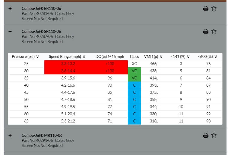
    The first rule of PWM nozzle selection is to understand that under average travel speeds, we’d like to see the duty cycle of the system at between 60 and 80%. This means that the nozzle solenoid is open about 2/3 of the time. This value also describes the flow rate as a proportion of the full capacity that nozzle.

    The reason for this 2/3 duty cycle rule is to enable four key features of PWM:

    1. It’s ideal for turn compensation, allowing the outer nozzles to increase their flow 20 to 40%, and the inner nozzles to decrease flow about three-fold, in accordance with boom speed.
    2. It allows speed flexibility, providing some additional speed, but more importantly, reduced speeds should conditions require it, without a change in spray pressure.
    3. It compensates for pressure changes so that spray quality can be adjusted without requiring a speed change. Less pressure reduces nozzle flow, and increasing DC recoups accordingly.
    4. It allows for customized higher flows of certain nozzles, perhaps behind wheels, to address reduced deposition in their aerodynamic wake (available on some PWM systems).

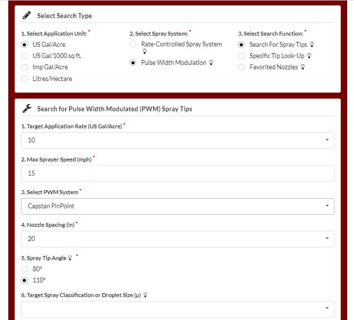
    The best tool for selecting the right nozzle size is Wilger’s Tip Wizard. This site asks for your desired average speed ( although it calls this “Max Sprayer Speed”), and reports the expected DC for a host of nozzle size solutions and pressures. It also reports maximum and minimum travel speeds and other useful information such as spray quality.

    Fig 1: The Tip Wizard is a useful tool for sizing nozzles on any PWM system. Sizing information applies to any nozzle. Spray quality information is for Wilger ComboJet nozzles only.

    Although intended for Wilger nozzles, the site’s sizing feature works for any nozzle brand. It asks the user which PWM system they have for the purpose of calculating the documented pressure drop across the solenoid.

    Fig 2: Tip Wizard results for the Wilger SR11006 tip at 10 gpa and 15 mph. Look for a solution that provides 60 to 80% Duty Cycle (DC).

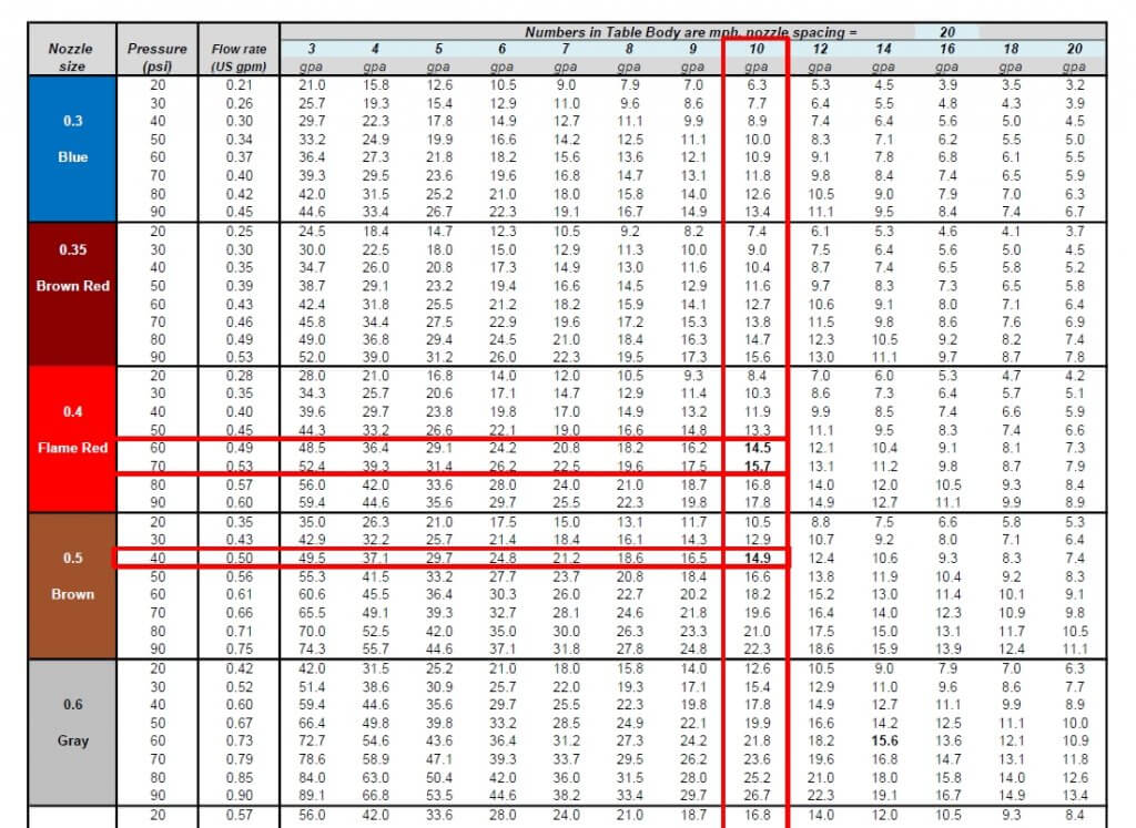
    If you don’t have access to the site, a basic calibration chart can still work with a simple trick. Recall that we use the top row to identify the desired water volume, and the table’s interior values are speeds, as described here.

    Below are two solutions for someone wanting to apply 10 gpa at 15 mph without PWM. The correct choice depends on the required pressure to produce the needed spray quality.

    Fig 3: A conventional calibration chart, solving a 10 gpa application for 15 mph.

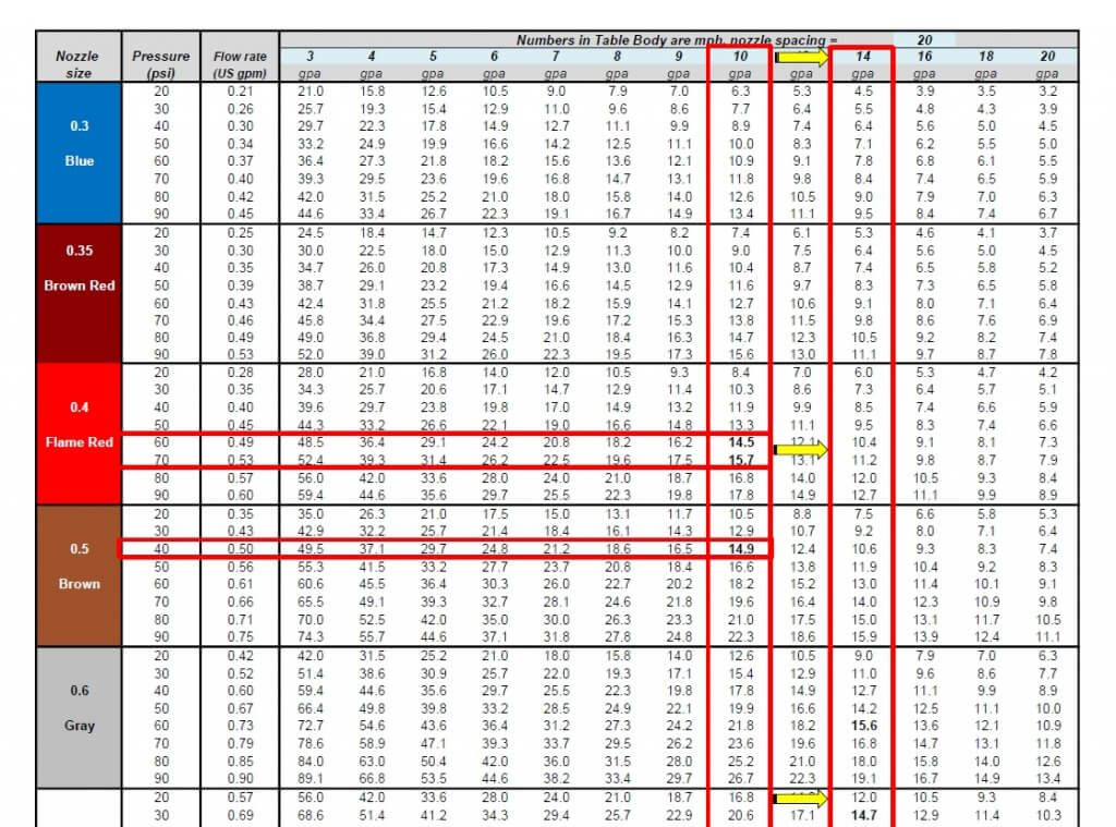
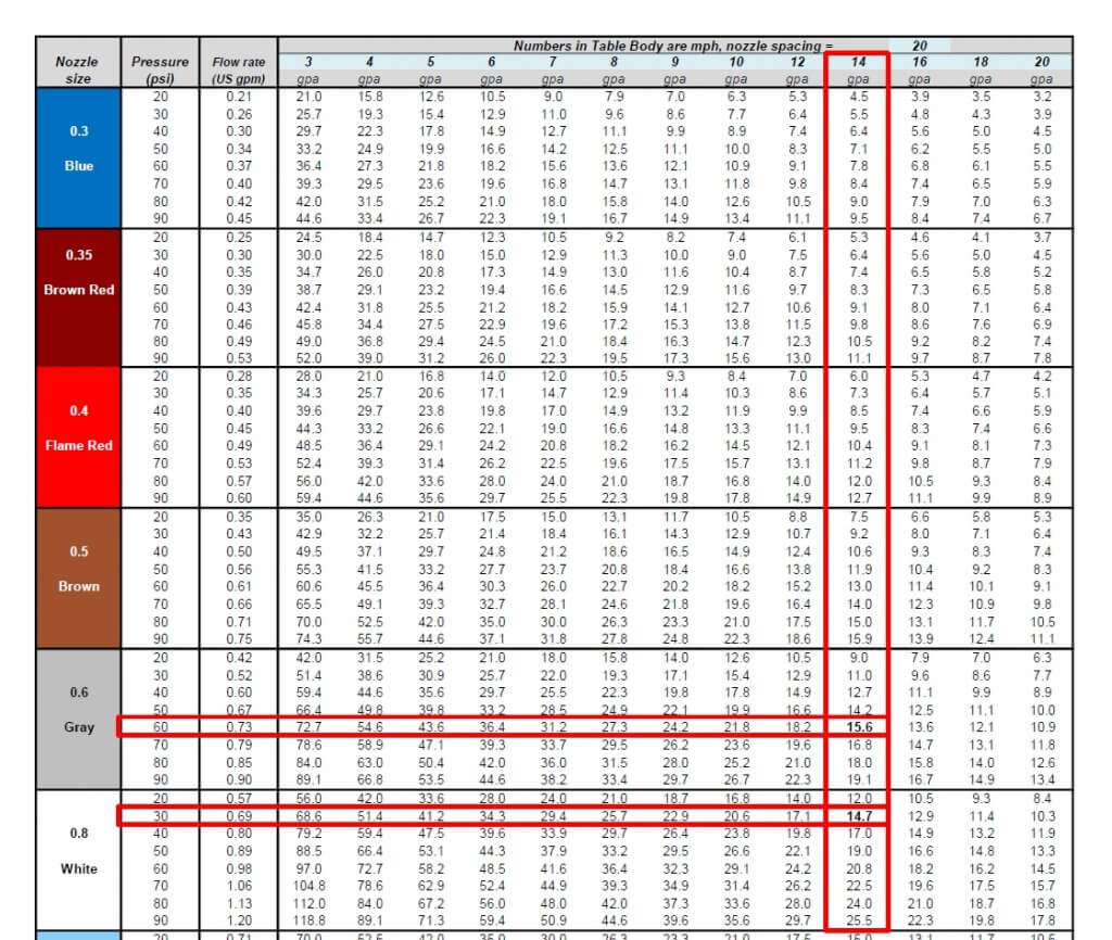
    If you want to apply the same 10 US gpa using PWM, simply solve for a larger volume that offers the right DC. For example, choosing 13 gpa will over-apply by 3 gpa, or 30%. The PWM system adjusts by running at 100-30=70% DC. If the chart doesn’t offer 13 gpa, go nearby, to 14 gpa, as we did below:

    Fig 4: By pretending to require 14 gpa instead of the actual 10 gpa, the conventional calibration chart is tricked into solving for a nozzle size that will work with PWM at 60% Duty Cycle.

    Now solve for the same target speed, 15 mph. The solution will run at 60% DC. Again, there is more than one choice, and that will depend on the spray pressure needed.

    Fig 5: Two possible solutions for achieving 10 gpa at 10 mph. An 06 nozzle at intermediate pressure or an 08 nozzle at low pressure.

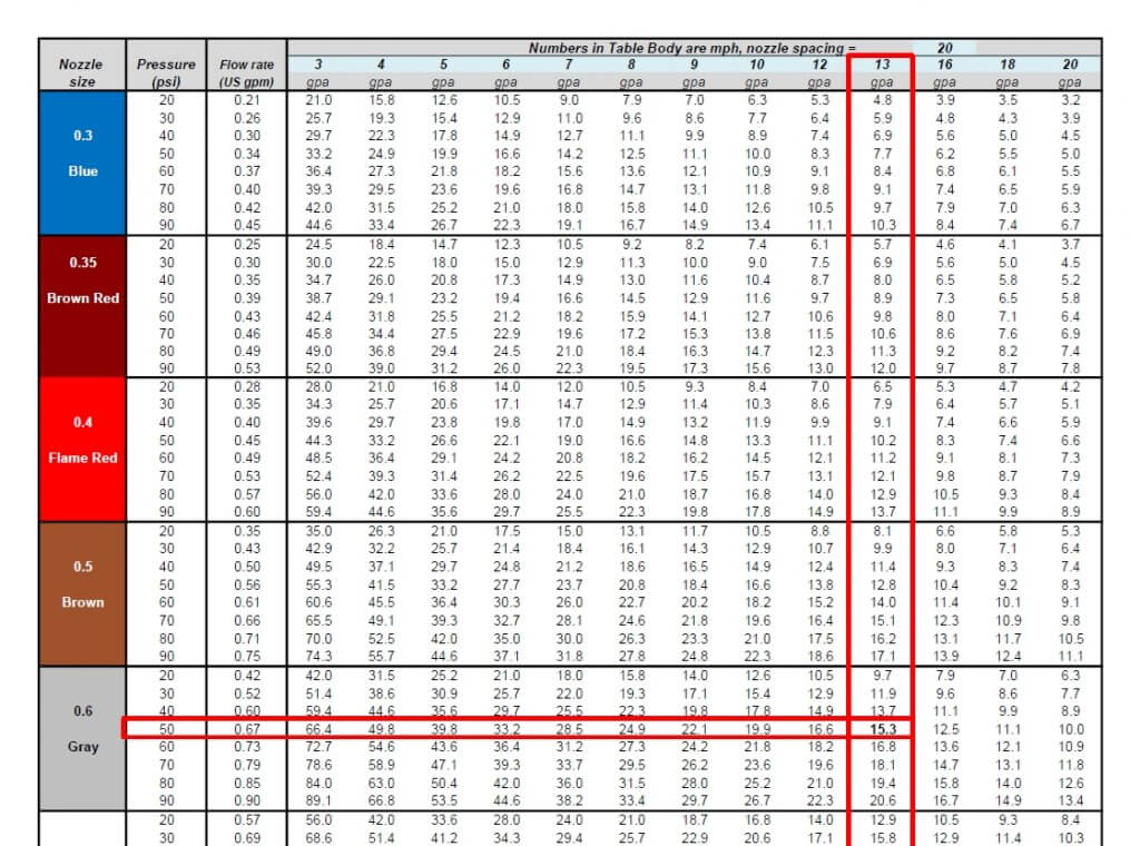
    We’ve developed a template, in US or metric units, that can be customized for any water volume. Here is the same chart with 13 gpa added:

    Fig 6: A conventional calibration chart with the 13 mph speed added.

    The best solution for 10 gpa at 15 mph is the 06 size nozzle at 50 psi. This is not engraved in stone. One of the nice things about PWM is that it has inherent flexibility. Make the nozzle pressure a priority to get the correct spray quality. It really doesn’t matter whether the resulting DC is 65 or 80%, the system will still work well. Simply avoid extremes that take you below 50% or above 90%, they will limit the system’s capabilities.

    The worksheet can be downloaded below:

    It can handle any water volume or nozzle spacing by filling in the blue cells. Two additional worksheets in the file automate the process, simply enter the desired application volume, travel speed, and nozzle spacing (yellow cells), and the solution that offers the optimal duty cycle range will be highlighted in light green.

  • Exploding Sprayer Myths (ep.13): Reading Nozzles and Nozzle Tables

    Exploding Sprayer Myths (ep.13): Reading Nozzles and Nozzle Tables

    After a long hiatus, it’s lucky episode 13!

    In this installment, Dr. Tom Wolf, intrepid reporter, braves the unforgiving wilds of Saskatoon as he investigates claims of mysterious devices popping up all over the city. Colloquially referred to as “nozzles” these items are imprinted with obscure codes that scientists are struggling to decipher. Be the first to learn how to read a nozzle and nozzle table in our newest installment.

    Want to know more about selecting nozzles? Check out this article and this one.

    Special thanks to the @RealAgriculture team and the Western Grains Research Foundation.

  • Dealing with Pesticide Shortages in 2022

    Dealing with Pesticide Shortages in 2022

    We’ve had dire warnings about possible pesticide shortages and price hikes for 2022. Price hikes are one thing. But if the products we need simply won’t be available, we have a tougher challenge.  It’s time to plan pesticide conservation.

    But first, what’s behind the product shortage?

    Emily Unglesby of dtnpf.com provided an excellent overview of the issue here and here. She said the reasons for the shortage are many-fold and came together in a perfect storm. Starting about 2017 or so, pesticide manufacturers tried to reduce the overall inventory of products to improve logistical efficiencies.  That effort was rewarded in 2019 when a wet spring in the US dramatically reduced seeded area to a low of 165 M acres. The resulting lower demand again provided incentives to reduce inventories. At the same time, US trade sanctions against China in the form of tariffs impacted production and shipment of many active ingredients to US markets. When Covid-19 happened, it affected both production and shipping of many goods, including pesticides. Container shipment costs increased sharply, and the ability to move them to and from ports was hampered. This then coincided with record seeded area in the US of 180 M acres in 2021, creating higher than usual demand. By that time, very little buffer remained in the system. The growth of Enlist E3 and Xtend Flex has placed additional pressure on glufosinate.

    Then two further events occurred. Hurricane Ida forced a shutdown of Bayer’s Louisiana glyphosate plant. And China, in late 2021, legislated a temporary 90% reduction of yellow phosphorus production in Yunnan Province in anticipation of the 2022 Olympic Winter Games. With phosphorus as a fundamental ingredient in glyphosate, glufosinate, and some fertilizers, this loss of production places significant strain on many products. The usual habit of returning unused pesticides to the retailer also became less common amidst shortage news, adding difficulty to planning inventories and demand.

    Shortages of popular herbicides like glyphosate, glufosinate, and clethodim will put demand on alternatives. Spreading out risk by implementing pre-emergent products where possible will pay dividends. But the ability to ramp up production of minor products is just as dependent on the supply chain, and these alternatives may therefore not offer reprieve if ordering is left to the bitter end. Planning ahead and staying in touch with retailers about your plans and your own inventory will assist the entire system in managing production and redistributing existing stocks.

    Safe to say products will be more expensive, and possibly impossible to obtain. Here are some things to consider to minimize the impact.

    1.Grow crops that require less pesticides. Crops which have good genetic resistance to insects and disease will be more likely to cope without a protective spray. Some crops are inherently competitive early on and give less time and space for weeds to become established. Remember that the relative time of emergence is important for crop yield loss from weeds. If crops emerge before weeds, they have the upper hand and will maintain higher yield potential. Crops that can be seeded early will prevent weeds from occupying that niche.

    A competitive crop is the best herbicide.

    2. The most powerful herbicide is a competitive crop. Use agronomic tools that favour good seedling establishment. The usual advice of seeding into a warm, firm, moist seedbed, should we be fortunate enough for the weather to cooperate, applies here. There is value in higher seeding rates to help outcompete weeds. Use fertilizer placement that favours crops, not weeds, such as side banding.

    3. Sample the spray water source and have it professionally tested. After a record drought in western North America, aquifers are low and surface waters have receded. Water quality will probably not be the same it has historically been. Use water conditioners to reduce effect of hard cations and bicarbonates. Ammonium Sulphate (21-0-0-24) at 1% w/v is a general treatment, harder water may require up to 3%.

    Conduct a water test in 2022 and condition spray water if necessary.

    4. Do not use untested mixes of pesticides with specialty foliar fertilizers. These may impact herbicide performance, or worse, result in an incompatible mix.

    5. Use the lowest label rate of product that is relevant for the pest you’re trying to control. Many products have a range of rates depending on the weed species and stage. Scout your fields and take advantage of the lower rate option if you can.

    Invest in logistics and be prepared to respond to a good spray day to get the timing right.

    6. Spray herbicides early. It’s been shown that crop plants can sense the presence of weeds before they compete for resources, causing a physiological adjustment that results in irreversible yield loss. The shorter the time that weeds and crops co-exist, the better. Also, smaller weeds are easier to control. Weeds that escape this early application will need to compete with an established crop and won’t thrive or impact yield as much.

    Smaller weeds are easier to control and may allow a lower label rate.

    7. It’s not advisable to reduce product rates from the one recommended on the label. Although label rates contain a margin for poor conditions, the risk of selecting for polygenic resistance exists. Polygenic resistance occurs when some weeds happen to be slightly more tolerant to the herbicide than the rest of their cohort. These weeds may survive a lower rate, and go on to produce seeds. If these outcross with other survivors, their more tolerant offspring will increase in relative abundance. With further such selections in subsequent generations, weeds become even more tolerant and eventually dominate.

    8. Apply the spray as uniformly as possible. Make sure the spray nozzles are within a 5% flow rate tolerance along the entire boom. If the set is older, consider a wholesale replacement. But the biggest enemy of uniform deposition seems to be turbulence created by wind and driving speed around the tractor unit. Slower wind and travel speeds help somewhat. Variable deposition means that some regions receive up to 50% more than intended, and others receive 50% less. This means weeds in the lower deposit regions may survive the application. The more variable the application, the higher the rate that is needed for acceptable control.

    Slower travel speed reduces variability of the spray deposit, limiting escapes.

    9. Use finer sprays whenever the tank mix contains a contact mode of action product (e.g., Group 1, 6, 10, 14, 15, 22, 27) or targets grassy weeds. Both situations require smaller droplets for best performance. The use of finer sprays may mean fewer hours in the day when drift is acceptable, and as a result, investment in efficient tendering and cleaning as well as overall time management pays dividends.

    10. Make efficient use of the product in the tank, preventing waste. The amount of product being discarded can range to over 10% of the total needed to treat a field, but this can be reduced to 3% with the proper steps. The following are areas where improvement is possible:

    (a) Prime the boom efficiently using sectional shutoffs or better yet, a recirculating boom. These can be primed without any spray leaving the nozzle or boom ends.

    Conserve product by eliminating priming waste with a recirculating boom.

    (b) Measure the spray mix of the last tank accurately, minimizing leftover. Consider the AccuVolume system that weighs the tank contents to the closest gallon. Tanks can be filled with the exact amount, and rates can be adjusted as the leftover becomes apparent on the last passes.

    Accurate measurement of tank volumes prevents leftovers.

    (c) Invest in individual nozzle shutoffs to improve sectional control resolution. These are part of any Pulse Width Modulation system but can also be obtained as air-actuated valves that are very affordable. Such capability is necessary for recirculating booms.

    Nozzle sectional control can save 4 to 5% product use.

    14. Consider an optical spot spray system such as the WEEDit Quadro, the Trimble WeedSeeker, or the John Deere See & Spray Select, available for 2022. These systems are “Green on Brown”, meaning they selectively spray just weeds in a burnoff or chem-fallow. This can save about 70% of the spray depending on weed density. More such systems are on the way, some even offering “Green on Green” that selectively identifies weeds among a crop. The return on investment of these systems is directly related to the pesticide cost, meaning in a year with high pesticide prices they pay off faster. If shortages of product become a reality, a spot sprayer may be the only way that some fields get treated at all.

    Pesticide shortages will not be fun. Unfortunately, their appearance coincides with higher fertilizer prices, meaning crop establishment will need to overcome that factor as well. But there are tools to minimize the impact if we’re willing to implement them. Just as necessity is the mother of invention, scarcity is the father of conservation.

  • Pressure Changes Spray Angles

    Pressure Changes Spray Angles

    When we consult a nozzle catalogue we are interested in the flow and droplet sizes produced at a given pressure. Perhaps we should also consider the effect of pressure on spray angle. We have several articles discussing the collective impact of spray overlap, nozzle spacing and boom height on coverage uniformity (Check here and here for example). However, we don’t really address the fact that fan angle is not a constant. This may be more relevant with the growing adoption of spot sprayers.

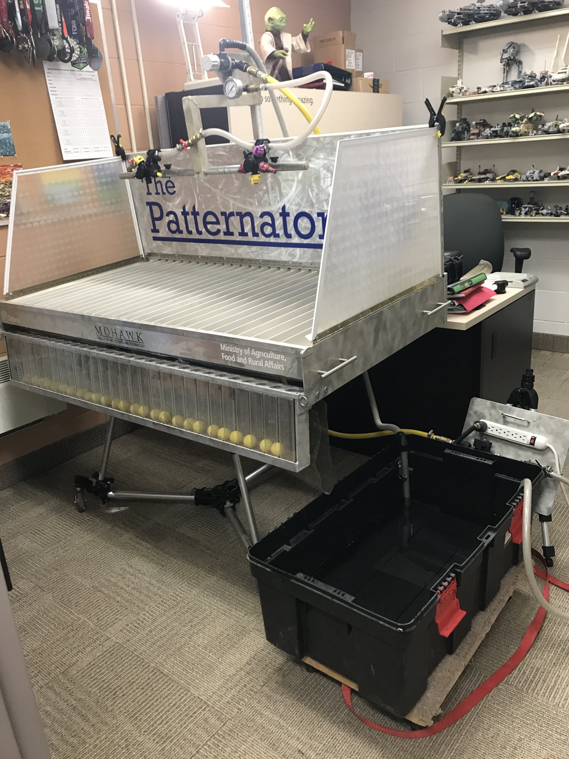
    To illustrate the potential for fan angle variation, we assembled a collection of red, flat fan nozzles (‘04s) from several manufacturers. We plugged each nozzle into a spray pattern table, set the regulator at a given pressure, and photographed the spray angle and flow distribution. This process was repeated for each nozzle at seven different pressures within the manufacturer’s approved range of 20-80 psi. After digitizing the photos, we measured the spray angle using a digital protractor.

    We anticipated a concomitant increase in spray angle as the pressure increased. This is not news. Anyone who has operated a sprayer has seen the spray pattern open up as the boom fills and pressurizes. Bear in mind this was only performed once (i.e. n=1), so while it illustrates trends it shouldn’t be mistaken for a rigorous scientific comparison. Further, this demonstrates a static situation and not a dynamic one where travel speed, wind conditions and the vortices from the sprayer it self will influence matters.

    We saw similar trends with nozzles other than 110˚ fans, but let’s focus on 110˚s due to their current popularity.

    Fan angles for five common 110 degree AI flat fans over their manufacturer-recommended pressure range
    Fan angles for five common 110 degree AI flat fans over their manufacturer-recommended pressure range

    The spray angle for 110˚ nozzles ranged from 75˚ at 20 psi to approximately 143˚ at 80 psi. One nozzle failed to reach 110˚ at any pressure. Conversely, there was another that was over 110˚ at nearly all pressures. Ideally, spray nozzles should be operated around the middle of their manufacturer-recommended operating range. Three of the nozzles tested came close to 110˚ at that median pressure, but only the TeeJet AIC110-04 measured 110˚ at the middle of its recommended range (~50 psi).

    Using that nozzle as an example, let’s look at the pressure, spray angle and subsequent distribution of flow along the swath at three different pressures. At 20 psi, the spray angle was 85˚. The yellow balls are floats that reflect flow as a series of cross sections of the swath. We see that aside from the tapered edges (which illustrate the need for 100% overlap between neighbouring nozzles) the distribution was fairly even. One of the priorities in nozzle design is to ensure a low coefficient of variability over the operating pressure range. In other words, the length of the swath may change, but the spray quality and uniformity in that swath is still within spec. At 50 psi the nozzle produced the expected 110˚ fan, and the spray distribution remained even. At 80 psi, the angle spread out to 125˚, spanning a greater distance, but it started to produce a less-even distribution.

    Photographs of spray angle and distribution for the TeeJet AIC110-04 at the extreme low, middle and highest pressures of its recommended pressure range.
    Photographs of spray angle and distribution for the TeeJet AIC110-04 at the extreme low, middle and highest pressures of its recommended pressure range.

    When fan angle changes with pressure, it can have significant implications. Nozzle spacing on a boom varies from sprayer to sprayer. Generally 50 cm (20 inch) centres are the standard in North America, but we’ve seen 15″ and even 10″. Nozzle spacing and boom height collectively determine the degree of spray overlap. Excessive overlap isn’t a problem, although additional nozzles do mean added expense, cleaning time and potential for plugging. Conversely, gaps in the pattern could lead to sub-lethal applications or flat-out misses. For example, in this soybean demo plot (below) we sprayed a contact herbicide at low pressure to collapse the spray pattern. You can see the alternating stripes of hits and misses that resulted from an incomplete overlap of spray.

    Soybean demo plot sprayed with a contact herbicide using 110 degree air induction flat fans at 20 psi. The collapsed spray pattern did not overlap sufficiently to burn the entire crop down, leaving a striped pattern and demonstrating the poor coverage.
    Soybean demo plot sprayed with a contact herbicide using 110˚ air induction flat fans at 20 psi. The collapsed spray pattern did not overlap sufficiently to burn the entire crop down, leaving a striped pattern and demonstrating the poor coverage.

    Nozzle manufacturers generally recommend a 100% spray overlap for flat fans. This creates sufficient overlap when the boom sways low to the ground. It also increases the degree of droplet size homogeneity under the boom as coarser and fewer droplets are generally found at the “horns” or edges of the pattern compared to the centre. In order to ensure this degree of overlap, sprayer operators should observe and consider changes in fan angle over their typical pressure range. Otherwise, the cost of poor deposit uniformity under the boom could be high.

    • Operate nozzles around the middle of the manufacturer-recommended pressure range. However, just because a nozzle is rated over a range of pressures does not mean the angle is constant.
    • Lower pressures are a greater concern than higher pressures. 30 psi is the absolute lowest pressure for operating a 110˚ air induction flat fan; the ideal operating range for these nozzles is 50-70 psi.
    • If nozzles are not maintaining the recommended 100% overlap at your preferred pressure range, then consider switching nozzle rates, and adjusting pressure and boom height.

    This work was performed with Victoria Radaukas, 2015 OMAFRA application technology summer student.