In this parody of SCTV’s Tex and Edna Boil we have some tongue-in-cheek fun while reminding people to maintain a healthy skepticism when reading RPAS marketing materials. Always be sure to ask questions and see the data before you believe what might be too good to be true.
Special thanks to Jason Strove for his masterful post-editing magic.
This work was performed with contributions from Adrian Rivard (Drone Spray Canada) and Adam Pfeffer (Bayer Crop Science – funding partner). Dr. Tom Wolf is gratefully acknowledged for his editorial support and assistance interpreting the results.
Introduction
This research is part of a continuing effort to identify best practices for broad acre crop protection using remote piloted aerial systems (RPAS). Previous work in wheat, corn and soybean has provided insight into how RPAS operational settings and environmental factors affect drift potential, effective swath width and spray coverage. This information, paired with advancements in RPAS design, has helped operators to improve spray deposit accuracy.
However, RPAS still produce what has traditionally been considered poor (or at least sporadic) broad acre coverage. Many studies have illustrated these shortcomings using herbicides or fluorescent tracers. Contributing factors include inappropriate operational settings, low application volumes (20-50 L/ha) paired with coarser spray qualities, and inaccurate swath widths. In light of these issues, we struggle to reconcile claims of acceptable disease control, which is arguably the greatest challenge in a spray-based crop protection paradigm.
Tar Spot
One real-world example of intermittent disease control from aerial applications (not just RPAS) is the case of tar spot in corn. Tar spot is a fungal disease caused by Phyllachora maydis and it is becoming a significant economic concern in Ontario. Left unchecked the disease causes rapid, premature leaf senescence. This reduces photosynthetic capacity, and ultimately, yield. Depending on spray timing, crop variety, environmental stressors, and the product applied, protection should last for up to three weeks.
In the last few years there have been several reports (both in Ontario and in corn-producing US states) of tar spot “striping” following aerial sprays. Crops seem well protected directly beneath the flight path (green and healthy), but efficacy tapers to failure towards the edges of the swath (brown and desiccated). Fundamentally, this is likely due to inadequate spray coverage caused by an overestimation of the effective swath width.
Figure 1 Tar spot striping in Western Illinois following two applications from a fixed wing sprayer (2023).Figure 2 Tar spot striping from RPAS volume trials. A brown strip can be seen between two passes in each RPAS treatment of 30 and 50 L/ha. The top is an application by a 100 foot horizontal boom. Each treatment is separated by an unsprayed check. (2023).Figure 3 – Tar spot striping in Ontario corn following fungicide application by helicopter (2024).
Effective Swath Width (ESW)
The measured swath width presents the lowest variability (as indicated by the coefficient of variability, CV) while minimizing the degree of over- and under-dosing. As a matter of operational productivity, wider swaths mean wider route spacing, which is attractive because it means fewer passes and faster applications. Once the agronomics are considered, the effective swath width is that portion of the swath that gives the desired biological result. It may equal, or only be a fraction of, the measured swath width. It is plausible that inappropriate effective swath widths from aerial applications are common, but have not always been detected, because:
Generally, fungicides are weakly systemic and give modest yield increases from disease suppression and their “stay green” properties. Until tar spot, a sub lethal dose of fungicide did not lead to rapid and acute crop failure.
Most growers do not intentionally leave unsprayed checks, or the check locations do not coincide with disease presence.
The applied product rate is sufficiently high to cover regions of under-application.
Taken together, deficiencies are often too subtle for passive detection.
This is not to suggest that pilots intentionally inflate swath widths. Swaths are evaluated during fly-in calibration sessions using established protocols (e.g., Operation S.A.F.E.), and RPAS swath evaluation has emulated these practices. Calibrations take place on bare ground or stubble/grass using two-dimensional samplers (i.e., continuous samplers like string or bond paper, or discreet samplers like water sensitive paper). However, this protocol does not account for any physical interference from the crop canopy itself. This may have negative implications, particularly given the unique nature of the RPAS swath.
RPAS tend to produce swaths with a very narrow span and a steep profile. To a certain extent, their swath widths share a direct relationship with altitude and headwind speed, and coarser sprays result in narrower swaths (with Dr. Michael Reinke, MSU). The outer edges of the RPAS swath represent the least amount of spray volume along the width, and this coincides with the turbulent dispersion zone of the downwash. Therefore, those extremes should contain a higher proportion of low-energy droplets moving in multiple directions relative the centre of the swath.
While crop morphology and planting architecture are contributing factors (i.e. part of the agronomic use case), it is generally accepted that the degree of spray penetration falls off exponentially with canopy depth. It follows that this should also be the case for any lateral movement, resulting in a significantly shorter swath in-canopy versus on bare ground.
Materials and Methods
Spray Sampling
Spray deposition was sampled using a 15.8 m (52 ft) Speed Track (Application Insight LLC) loaded with 3-inch bond paper (Staples Canada). The spray mix was 0.3% v/v FD&C Blue #1 Liquid. Bond papers were analyzed using a Swath Gobbler (2nd gen software – Application Insight LLC) at 100 mm sampling rate (i.e., ~150 discreet images per sample). Hue: 32-180. Saturation 17-60. Value: 156-255.
The Swath Gobbler produces a complete, correlated and ordered record of the cross-section of a swath. For each discreet image, it reports the number of individual droplet stains on the sampler per area. It also reports percent area covered by measuring the total number of pixels with dye divided the total number of pixels in the image.
The device deliberately does not calculate a Droplet Size Distribution (DSD) of the stains. This is because any DSD calculated from paper collectors relies on assumptions that cannot be validated, such as the fact that all droplets are captured and detected, spread factors are known for that application condition and similar for all stain sizes, there are no multiple hits, etc.
RPAS
The sprayer was a DJI T40, calibrated according to the pilot’s standard operating procedure (Drone Spray Canada). Certain operational settings varied with treatment and will be detailed later in this section.
The flight path was perpendicular to the sampler, aligned with the centre using pin flags as references for the pilot. Spraying began approximately 20 m prior to the sampler to ensure the RPAS was at target speed and continued some 20 m past the sampler.
Figure 4. DJI T40 approaching sampler on bare ground. Sampler was later moved into the adjacent wheat field (left).
Defining Coverage
Swath width will be calculated from two different coverage metrics.
Percent Area Covered describes the amount of surface area covered by deposit. Given the variable degree of stain diameter (a function of sampler material, spray mix, and droplet velocity) this value can only be used as a relative index (i.e., can only be compared to itself). No conclusions can be drawn about how spray interacts with plant tissue, but generally more coverage correlates to improved crop protection.
Deposit Density describes the number of individual droplet stains on the sampler per area. Higher densities can imply more uniform distribution over the plant surface, which is particularly important for contact materials.
Previous studies (with Dr. Tom Wolf, Agrimetrix Research and Training, data not shown) indicate a higher correlation between deposit density and swath width at lower versus higher spray volumes. Lower volumes are typically comprised of finer droplets, which are more accurately resolved using deposit counts. Swath widths determined by deposit density also tend to be longer than those determined using percent coverage, better aligning with real-world observations of efficacy.
Wheat
R40 wheat was planted on October 9th, 2023, at 808,000 seeds/ha (2 million seeds/ac). Wheat height at the time of the trial was 60 cm (25 in). The location was 45180 Fruit Ridge Line, St. Thomas, Ontario. Deposition trials took place on May 23rd. Wheat stubble swath testing also took place at this location on May 15th.
The RPAS was programmed to apply 50 L/ha using a 260 µm droplet diameter according to the DJI software. Air speed was 5 m/s and the flow rate was 11-12 L/min as it passed over the sampler. Swath was programmed at 8 m.
Coverage was evaluated for water (control) and for a spray mix containing 0.15% v/v Interlock (a drift mitigating adjuvant – Winfield United) and 0.15% v/v Interlock + 0.125% v/v Activate Plus (a spreader adjuvant – Winfield United). For bare ground, each treatment had three passes (n=3) except for water, which had four (n=4).
The wheat canopy was only sprayed with water three times (n=3). Limited passes were made because it served as a proof of principle. Any indication of relevant differences in the swath width would justify later trials in corn and soybean. These first passes revealed issues with the experimental design that were later corrected:
The RPAS spray tank level was not held constant. The RPAS weight affects the intensity of the downwash. The volume dropped from 30 L to ~20 L over the course of the experiment. In future trials, a tank volume of 20 L was maintained from a premixed source.
The wind direction occasionally shifted from a direct headwind to a partial cross wind from the RPAS’s right. In future experiments, we waited for an optimal wind direction before starting each pass.
The RPAS altitude was set to 3 m above bare ground. We assumed it would climb to account for the height of the wheat, but the canopy did not register with the RPAS sensors. As a result, spray was released ~60 cm closer to the wheat heads than to the ground in bare ground swathing. In future experiments, we confirmed that the RPAS was 3 m from the top of the crop canopy.
Despite best efforts, moving the sampler into the wheat parted and distorted the canopy. As a result, the sampler was not as obscured as it should have been. We developed strategies to minimize canopy distortion in corn and soybean that will be described later.
Figure 5. Top-down view of sampler in wheat canopy. Note that the canopy did not close over the sampler as intended.
Corn
Corn was planted on May 15th, 2024, at 13,300 seeds/ha (33,000 seeds/ac). The sampler was erected in the field on July 3 to allow the canopy to grow up and around it. Deposition trials took place on July 26 and every effort was made to leave the canopy undisturbed around the sampler. Corn measured 2.4 m (9 ft) at the tassel and 1.2 m (4 ft) at the silks. The sampler height corresponded to the ears. The location was 42°40’52.1″N 81°04’45.9″W near 5277 Quaker Road, Sparta, Ontario.
Figure 6 Sampler erected to 4 ft. Crop grew around the sampler to minimize any canopy disturbance.Figure 7 Sampler position relative to ears during sampling.Figure 8 Installing Speed Track for swath testing in wheat stubble.
Soybean
Soybean was planted on June 30th, 2024, at 80,800 seeds/ha (200,000 seeds/ac) on 38 cm (15 in) centres. Deposition trials took place the morning of August 14. While the densest area was selected for the trials, the field was patchy with crop height spanning 20-25 cm (8-14 in). Each section of the Speed Track was inserted under the canopy separately to avoid disturbing or damaging the plants. The track was elevated ~10 cm off the ground. The location was at 42°46’50.4″N 81°08’20.8″W near 43900 Talbot Line, Central Elgin, Ontario.
Figure 9 Sampler in soybean.
Corn and Soybean Treatments
The following treatments were repeated three times in-canopy (n=3) (Table 1). The actual flow rate (recorded as the RPAS passed over the sampler) was always ~1.5 L/min less than programmed.
Treatment #
Droplet Diameter (µm)
Programmed Swath (m)
Volume (L/ha)
Rate (L/min)
Flight Speed (m/s)
Spray Mix
1
320
10
20
10.5
10
water
2
320
8
30
10.5
8.3
water
3
320
8
50
10.5
5
water
4
320
8
30
5.7
5
water
5
500
8
50
10.5
5
water
6
320
8
50
5.7
5
0.5% Masterlock
7
320
8
30
10.5
8.3
0.5% Masterlock
Table 1 RPAS operational settings for corn and soybean treatments
The following treatments were repeated three times on wheat stubble (n=3) (Table 2). Once again, the actual flow rate (recorded as the RPAS passed over the sampler) was always ~1.5 L/min less than programmed.
Treatment #
Droplet Diameter (µm)
Programmed Swath (m)
Volume (L/ha)
Rate (L/min)
Flight Speed (m/s)
Spray Mix
1
320
10
20
10.5
10
water
2
320
8
30
10.5
8.3
water
3
320
8
50
10.5
5
water
4
320
8
30
5.7
5
water
Table 2 RPAS operational settings for wheat stubble treatments
Weather Data
The RPAS flight path was into the prevailing wind, but minor variations occurred throughout sampling. Weather was recorded as the RPAS passed over the sampler using a Kestrel 3550AG weather meter in a vane mount positioned on a tripod 2 m above ground (Table 3).
Terrain
Wind Speed (km/h)
Direction Relative to Flight Path
Temperature (°C)
Cloud Cover (%)
RH (%)
Bare Ground
3-5
Headwind +/- 25° from starboard
20-21
0
60
Wheat Canopy
5-7
Headwind +/- 25° from starboard
21-22
0
60
Corn Canopy
2-4
Headwind +/- 15° from starboard
23-26
<10
75
Wheat Stubble
4-7
Headwind +/- 15° from starboard
26-28
<10
65
Soybean
3-4
Headwind +/- 15° from starboard
22
0
55
Table 3 Average weather conditions during trials.
Results
Raw Coverage Expressed as Percent Coverage or Deposit Density
Coverage can be presented as raw data plotted by swath position. This is a qualitative means for assessing the swath. The bare ground data has been presented (using both coverage metrics) as an example (Figures 10 and 11).
Figure 10 Swath coverage data for water on bare ground expressed as percent area covered. All four passes are plotted.Figure 11 Swath coverage data for water on bare ground expressed as deposit density. All four passes are plotted.
Repetitions were similar enough to imply that environmental conditions were consistent during sampling. By averaging the repetitions, coverage in-canopy can be more easily compared to that on bare ground Figures 12 and 13).
Figure 12 Average swath coverage data expressed as percent area covered. Bare ground (n=10). Wheat canopy (n=3).Figure 13 Average swath coverage data expressed as deposit density. Bare ground (n=10). Wheat canopy (n=3).
The magnitude of coverage on bare ground exceeded that in-canopy, tapering to similitude and near-zero at the edges of the pattern. It can therefore be concluded that the entire swath was captured, and that spray was filtered by the canopy before reaching the sampler within.
The difference between bare ground and the wheat canopy was greater when the data were presented as percent area versus deposit density. Differences in the number of deposits from finer sprays were more accurately resolved using deposit density than percent coverage. Since it can be expected that smaller droplets penetrate a canopy better than coarser droplets, it may be more appropriate to use deposit density to document their presence. We also saw indications of wider swaths when data were presented as deposit density, as well as a bimodal distribution that reflected the positions of the two rotary atomizers.
While informative, this raw coverage format did not allow empirical comparisons. Each pass must be converted to a swath width.
Converting to Swath Width
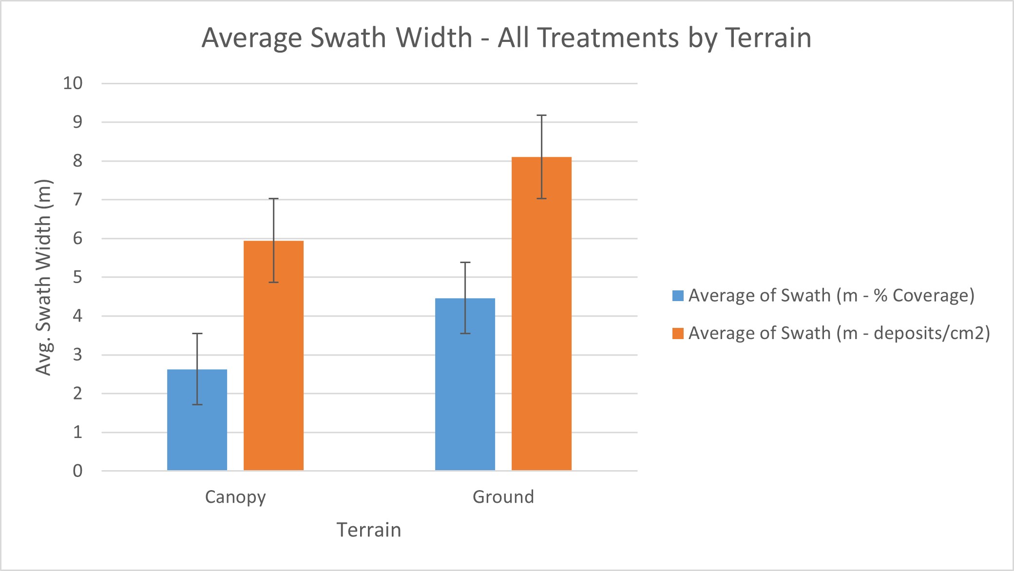
Each pass was transformed by averaging Swath Gobbler data to a single value every 0.5 m. Data were then entered into the www.sprayers101.com swath width calculator and the SW was manually determined for each pass. Criteria was the lowest overdose, lowest underdose and lowest CV for an idealized threshold coverage of 90% that of the highest value in the swath. In the following histogram, the SW from all treatments have been averaged for ground and canopy terrains (Figure 14).
There was a significant reduction in swath width in a wheat canopy compared to stubble or bare ground. There was a 41.2% reduction in swath width in a canopy when measured as percent area covered and a 26.6% reduction when expressed as deposit density. As previously stated, deposit density better reflects the contribution of finer deposits, which tend to penetrate deepest into crop canopies.
Figure 14 Average effective swath width for all treatments on all terrains. Swaths expressed from both percent coverage and deposit density metrics. Standard error bars presented. Canopy (n=45). Ground (n=22).
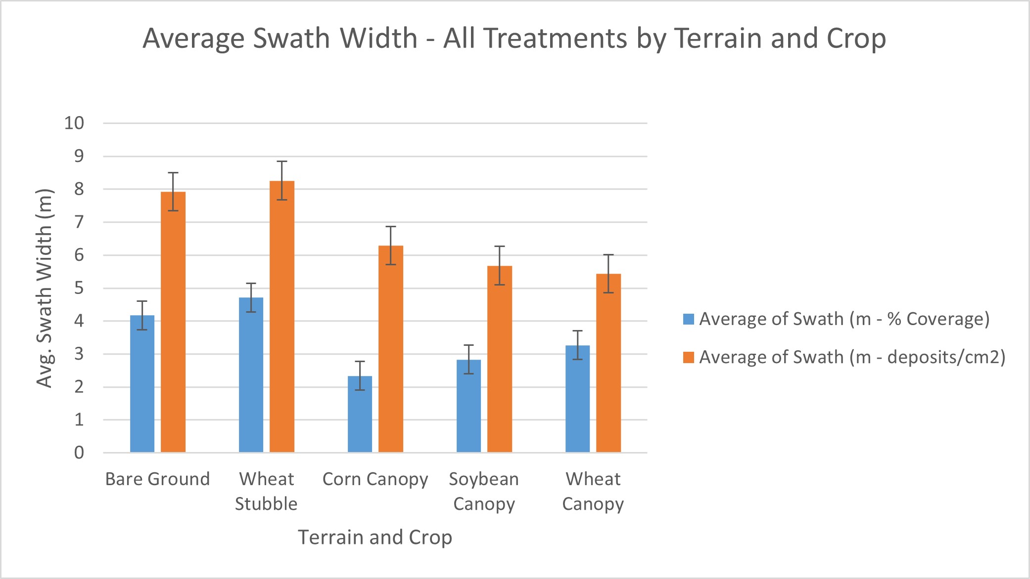
When the data is considered by terrain and by crop, we see that swathing on bare ground or in wheat stubble doesn’t have a significant impact. This justifies combining those data as “Ground” in subsequent analyses.
Another observation that supports the use of deposit densities is the difference between the intended (i.e., programmed) swath width and the detected swath width on ground (Figure 15). The SW on ground was closer to the intended 8 or 10 m swath width when expressed as deposit density. It was approximately half the desired width when expressed as percent coverage, which is considerably less than common practice.
Figure 15 Average effective swath width for each crop and terrain. Swaths expressed from both percent coverage and deposit density metrics. Standard error bars presented. Ground 8 m swath (n=19). Ground 10 m swath (n=3). Canopy 8 m swath (n=39). Canopy 10 m swath (n=6).
Canopy Effect
By percent area, corn had the biggest reduction in swath width compared to bare ground, then soybean, then wheat (Table 4 and Figure 16). This suggests the SW shares an inverse relationship with the canopy depth. However, the relationship reversed when SW was expressed as deposit density. The relationship between droplet size, crop physiology, planting architecture and canopy penetration is complicated, and no conclusions can be drawn beyond a reduction in SW in-canopy.
Crop
% Reduction in SW (% area)
% Reduction in SW (deposits/cm2)
Corn
44.0
20.6
Soybean
32.2
28.3
Wheat
21.7
31.5
Table 4 Reduction in average effective swath width in-canopy by crop compared to on ground. Swaths expressed from both percent coverage and deposit density metrics.
Figure 16 Average effective swath width for each terrain. Swaths expressed from both percent coverage and deposit density metrics. Standard error bars presented. Bare ground (n=10). Wheat Stubble (n=12). Corn Canopy (n=21). Soybean Canopy (n=21). Wheat Canopy (n=3).
Effect of Volume on SW
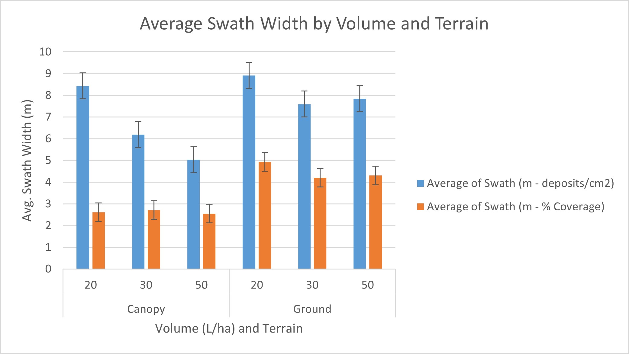
The effect of spray volume on swath width is not immediately clear. When the data were expressed as deposit density, volume shared an inverse relationship with SW in canopy (Figure 17). There appeared to be no effect when expressed as percent coverage. The inverse relationship is weakly expressed, if at all, for both metrics on bare ground.
Figure 17 Average effective swath width by volume and terrain. Swaths expressed from both percent coverage and deposit density metrics. Standard error bars presented. Canopy 20 L/ha (n=6). Canopy 30 L/ha (n=18). Canopy 50 L/ha (n=21). Ground 20 L/ha (n=6). Ground 30 L/ha (n=3). Ground 50 L/ha (n=13).
Effect of Speed on SW
For most RPAS designs, lower volumes are applied at higher flight speed (Table 5). Previous work demonstrated that higher flight speeds tended to result in wider swaths and an increase in drift. Do higher speeds cause wider swaths in-canopy, despite lower volumes?
Volume Applied (L/ha)
5 m/s Flight Speed
8.3 m/s Flight Speed
10 m/s Flight Speed
20
–
3 treatments
9 treatments
30
9 treatments
12 treatments
50
34 treatments
–
–
Table 5 – Number of treatments for each flight speed by volume applied.
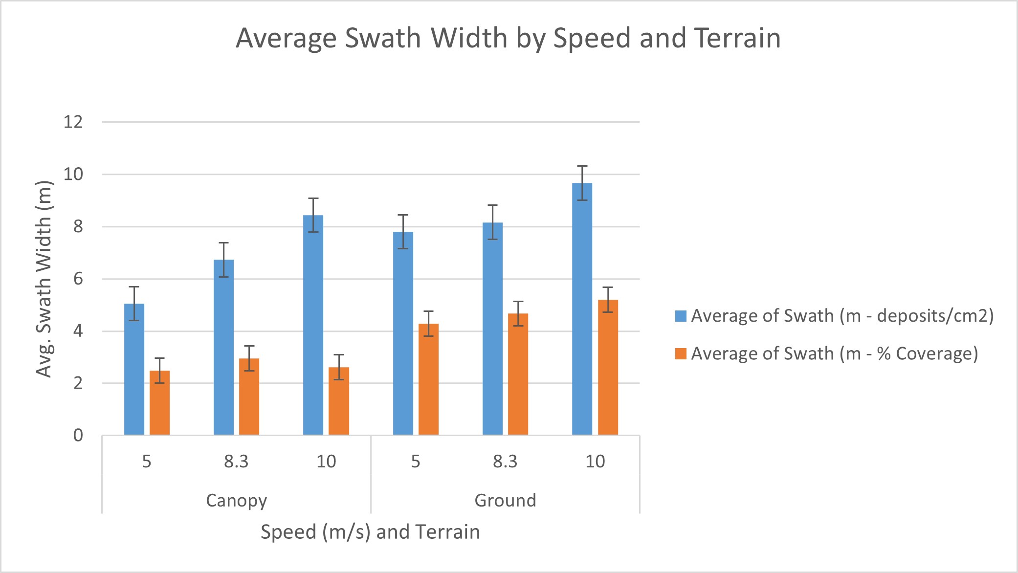
Flight speed had a clearer impact on swath width than spray volume did (Figure 18). There was a positive relationship between flight speed and swath width as measured by deposit density in canopy and on bare ground.
Figure 18 Average effective swath width by speed and terrain. Swaths expressed from both percent coverage and deposit density metrics. Standard error bars presented. Canopy 5 m/s (n=27). Canopy 8.3 m/s (n=12). Canopy 10 m/s (n=6). Ground 5 m/s (n=16). Ground 8.3 m/s (n=3). Ground 10 m/s (n=3).
Just as with volume, there appeared to be no significant effect on swath width in either canopy when expressed using percent coverage. This was likely because finer sprays were better able to penetrate a canopy and deposit density is better able to resolve their presence.
Conclusions
There was no difference in SW between stubble and bare ground. The SW on-ground was far closer to the programmed 8 or 10 m swath width when expressed as deposit density.
There appears to be a significant reduction of SW in-canopy versus on-ground. A crop canopy created a 26.6% reduction when expressed as deposit density. Specifically, corn was -20.6%, soybean was -28.3%, and wheat was -31.5%. Previous work has demonstrated diminishing coverage with canopy depth in corn, but it is difficult to make comparisons between agronomic use cases (e.g. different planting architectures and plant physiologies).
When the data were expressed as deposit density, spray volume shared an inverse relationship with SW in-canopy, but the effect on SW on-ground was less clear. However, RPAS speed had a clear inverse relationship with SW in-canopy and strong trend on-ground.
It is understood that finer spray is better able to penetrate canopies. One reason is because finer droplets are able to become entrained the downwash. Another is simply mathematical advantage, given that finer sprays are comprised of exponentially higher numbers of droplets than coarser sprays, increasing the odds of deposition. Conversely, coarser droplets (which have the greatest influence on percent area covered), are more likely to impinge on the canopy structure before reaching the sampler. Deposit density appears to be the more accurate metric for calculating SW both on-ground and in-canopy.
The reduced SW in-canopy versus on-ground explains, in part, why striping is occurring in aerial corn fungicide applications. The route spacing reflects on-ground swath width, where it should reflect the shorter, ESW.
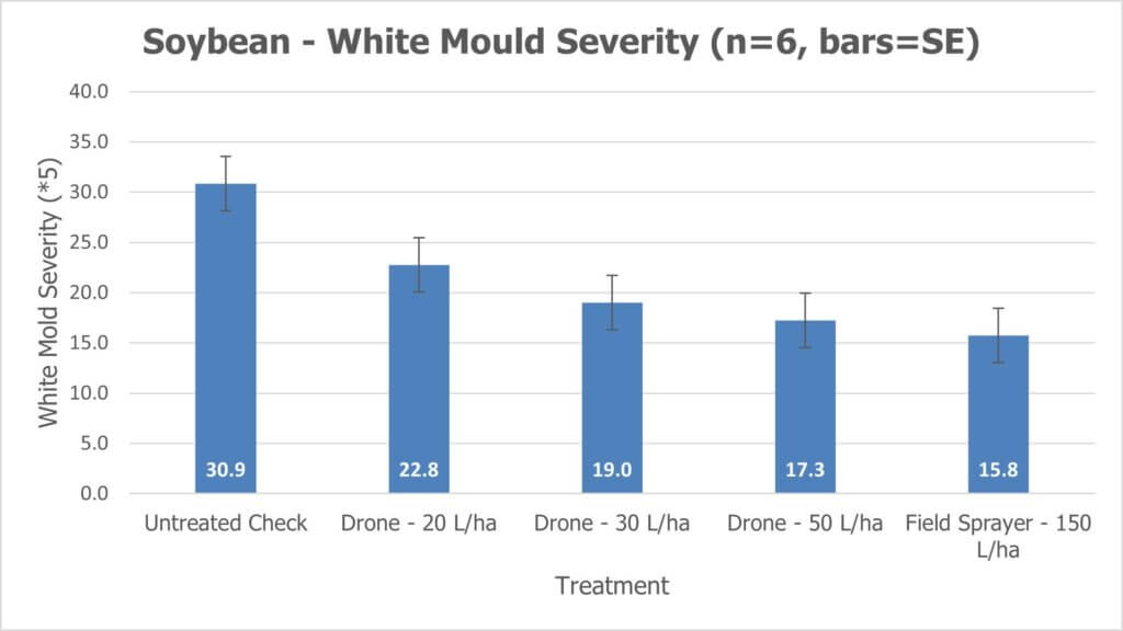
White mould is caused by the fungus Sclerotinia sclerotiorum and it’s an annual threat to soybean when cool, wet conditions correspond with flowering. Variety selection (e.g. high tolerance) and cultural control (e.g. crop rotation and wider row width) are important management tools, but ultimately the application of a crop protection product between R1 and R2 is required for high-risk fields. (Learn more here).
This article describes the results of an experiment exploring soybean canopy coverage and fungicide efficacy from a rotary spray drone. All work was performed under PMRA research authorization. There are currently no labels to apply crop protection products in Canada.
Experimental design
For the spray coverage trials, two locations were selected in southern Ontario (one south of Sparta and one west of Talbotville). This was a full field-scale trial with a single application made at R1.5 on July 18 (Sparta area) and July 22 (Talbotville area), 2023. There were two replications in each field and treatments were laid out parallel with the planting direction in a randomized design. Four other locations in Ontario and Quebec were also used in the larger efficacy/yield study. All locations had some level of white mould infection.
New Holland 345 – 150 L/ha (TeeJet XR11006 nozzles on 50 cm spacing) *Not included in spray coverage trial
We established an effective swath width of approximately 4 m (13.1 ft). The drone made three passes to cover the 12 m (40’)-wide treatment area, corresponding to the widths of the 9 m (30’) or 12 m (40’) headers later used to harvest in each field. Buffers were left on either side the treatment area. Fungicide was applied at label rate plus 0.125% Activate.
Target placement and retrieval
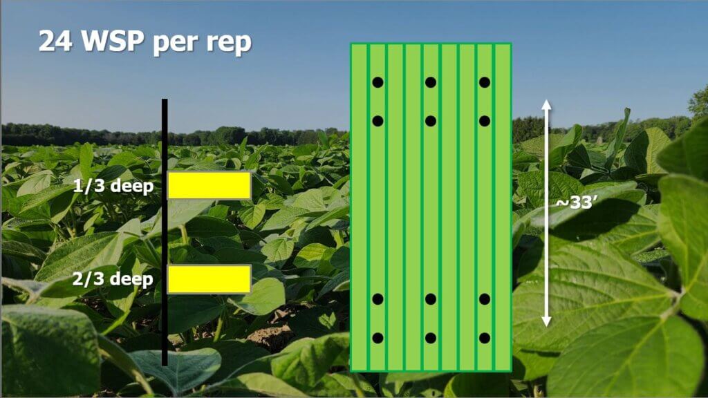
Soybeans were planted on 38 cm (15”) row spacing. The coverage sampling area was positioned in the middle of the treatment area. A length of rebar was positioned in-row and sheathed in PVC tubing. Two SpotOn brand water sensitive papers (WSP) from the same production run were secured face-up approximately 1/3 and 2/3 deep in the canopy. A block of six such samplers were positioned in a 3 x 2 grid (every third row and approximately 2 m apart in row). This block was then repeated 10 meters (33’) further into the block for a total 24 water sensitive papers per replicated treatment (see below).
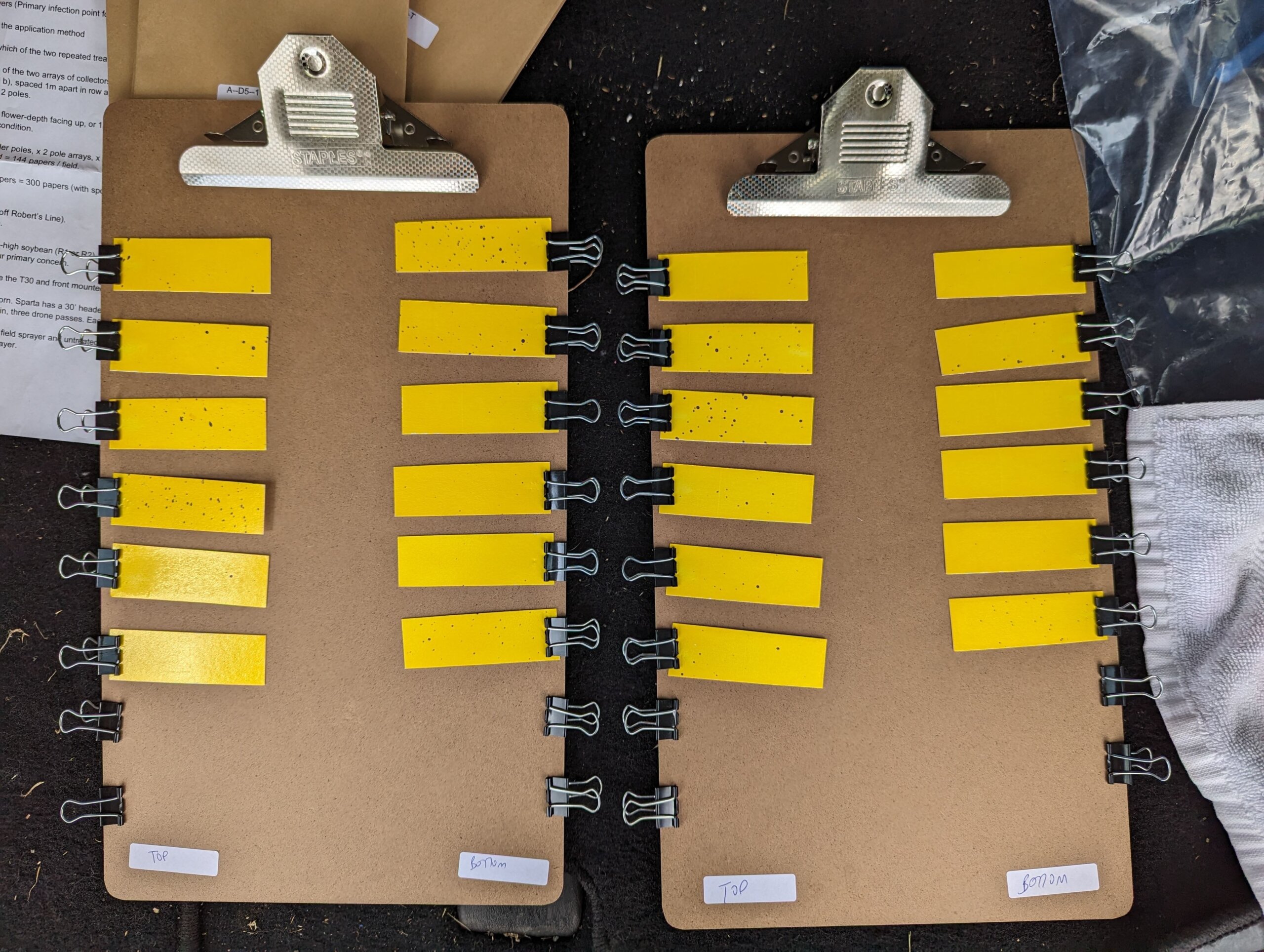
The papers were retrieved and temporarily placed on clipboards to dry before they were placed in paper bags for short term storage. They were digitized using a SprayX DropScope within 48 hours of retrieval on the “ground sprayer” setting, measured as percent surface covered (% area), and deposit density (# deposits/cm2).
Weather during coverage trials
Weather data was monitored using a Kestrel 3550AG weather meter (Kestrel Instruments) in a vane mount positioned 1.5 m (5 ft) above the ground. Wind speed fluctuated during the treatments, but wind direction remained relatively stable at 90 degrees to the flight path. The Sparta location averaged 6.4 km/h (4 mph) while the Talbotville location was considerably higher at 14.4 km/h (9 mph). Nevertheless, targets remained within the swath, despite any offset, as indicated by visual confirmation as well as the consistent coverage observed on the windward WSP compared to other, downwind samplers in each pass. Cloud cover was high at both locations.
Results
Coverage
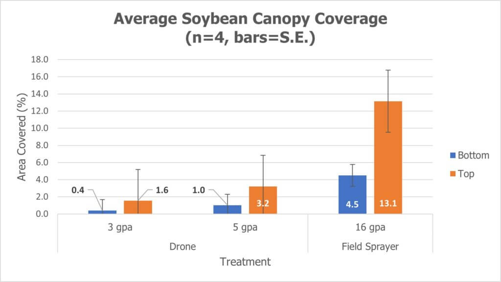
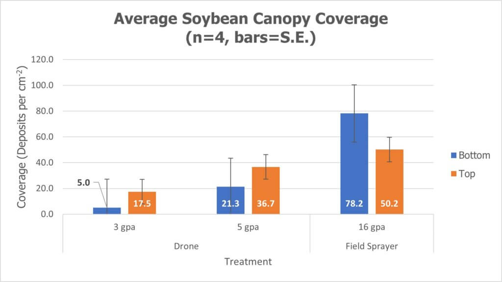
The coverage recorded from each WSP was averaged by canopy position (bottom 1/3 or top 1/3 of canopy) and presented in the following histograms with standard error. There were some spoiled collectors, primarily in the lowest canopy position, ruined by high humidity and physical contact with the plant. However, the lowest n for any treatment was 31 collectors and the highest was the full 48. Coverage is presented both as % area covered and as deposit density in counts per cm2.
Efficacy and yield
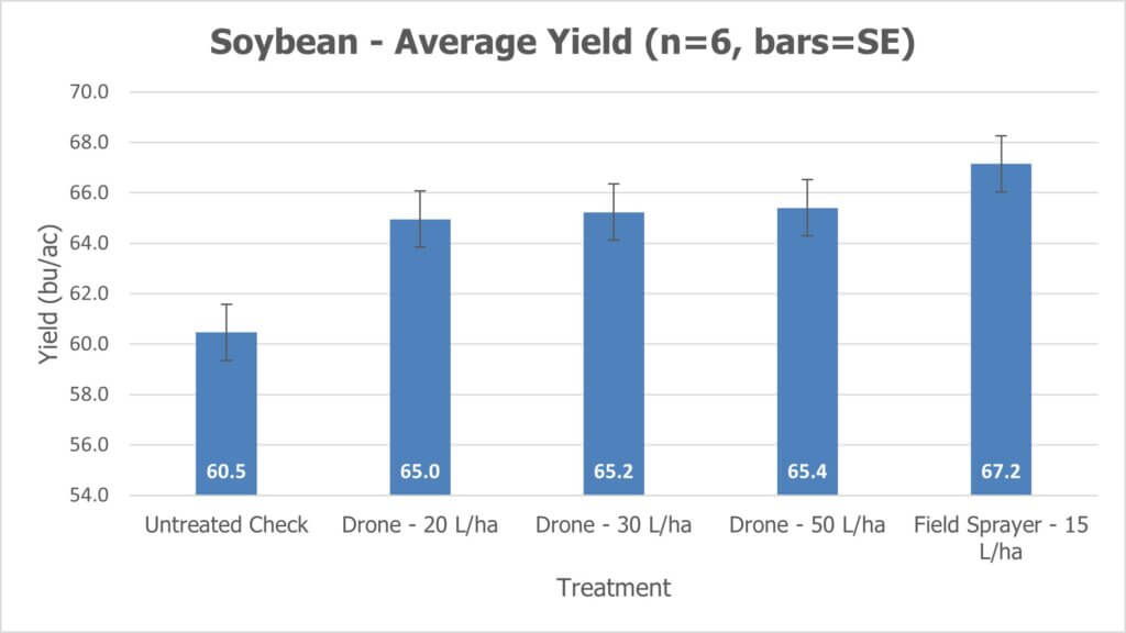
Three phytotoxicity ratings were performed 7, 14 and 21 days after treatment. White mould was rated at harvest and final crop yield reported in bu/ac.
Observations and Considerations
As expected, both water volume and canopy depth share direct relationships with percent-area covered (i.e. lower water and lower canopy depths mean lower coverage). Water volume also shares a direct relationship with deposit density for a given droplet size, but canopy depth is more complicated as smaller droplets tend to penetrate more deeply into canopies and low water volumes tend to produce smaller droplets. However, as a general observation, less water translates to less coverage no matter the metric for coverage, and this has been shown to reduce product efficacy.
How, then, can we reconcile the claims of efficacy from low-volume drone applications? It’s typical that the % area covered from a 50 L/ha drone application is ¼ or less than that of “conventional” field drop systems which in North America tend to employ 150-200 L/ha. In speaking with Mark Ledebuhr (Application Insight LLC) about how low volumes could possibly be efficacious, he explained that in sugarcane production in Guatemala, the condensing humidity is likely the reason why their 1 gallon/acre applications are working. The droplet survivability, and the re-hydration and secondary movement of the deposits were a good thing.
In the case of contact fungicides in North America, it may be humidity as well, but also the deposit density, combined with higher concentrations of active ingredient, that explain the similar efficacy and yields as seen here between the 50 L/ha (drone) treatment and the 150 L/ha (field sprayer) treatment. This would concentrate both the active ingredient (possibly increasing uptake rate, or residue persistence, depending on the product mode of action and the target’s physiology) as well as the adjuvant load (possibly improving sticking/spreading of deposits).
Another consideration surrounds how deposit spread is analyzed. Water sensitive paper underestimates the spreading effect that can occur on plant surfaces (especially where surfactants are used). This is why WSP tends to be used as a relative index, meaning that papers should only be compared to other papers. Perhaps deposits are spreading more on the plant surfaces in the low-volume drone application (again, given the higher concentration of formulated adjuvants) than the water sensitive paper is indicating, and that is improving efficacy.
This concept of how low-volume applications might affect coverage and subsequent efficacy, and the potentially positive impact of re-formulating products to include higher adjuvant loads, is well-described in this precis by Dr. Andrew Chapple and Malcolm Faers. Currently, accepting that the amount of control provided by the drone application falls short of that provided by a field sprayer, this study indicates that drones have the potential to produce acceptable results in fungicide applications if conditions are suitable, timing is optimal and water volumes are sufficiently high.
This study was a collaborative effort with Bayer Canada and Drone Spray Canada.
This article summarizes a 2022 paper that can be downloaded here.
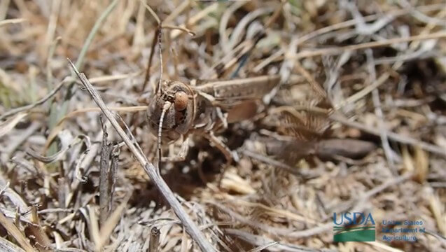
Grasshoppers are an integral part of rangeland ecosystems, but population outbreaks can cause significant damage to adjacent crops and forage. For example, cattle consume about 1.5-2.5% of their body weight in forage per day, so pound for pound, a grasshopper will eat 12-20 times as much plant material as a steer. This represents serious economic damage to the cattle industry, especially during times of drought when forage is already scarce.
Insecticides are the primary means for suppressing grasshopper populations, and they are typically applied on rangelands using conventional fixed-wing aircraft, per the United States Department of Agriculture (USDA) Animal and Plant Health Inspection Service (APHIS) Rangeland Grasshopper and Mormon Cricket Suppression Program. This is particularly effective when population hotspots can be targeted before those populations grow to critical numbers, but depending on the location, this short turn-around time can be challenging.
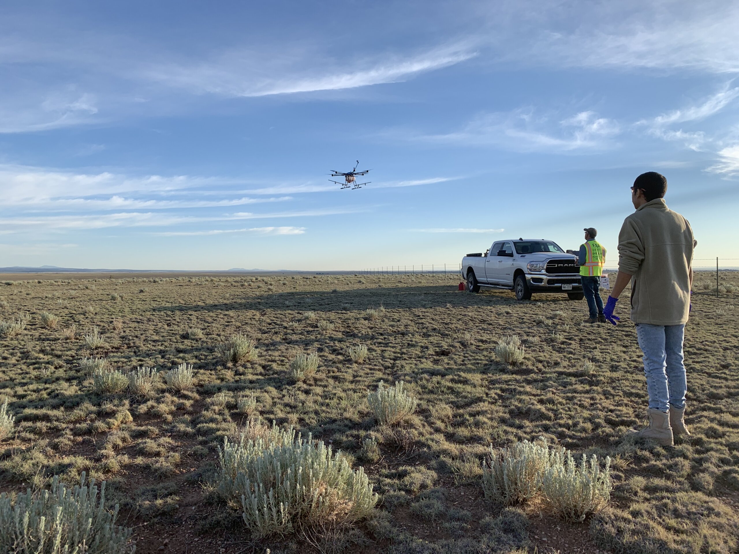
Recently, the use of remote piloted aerial systems (RPAS or drones) for spraying in small farm operations and for site-specific management of crop pests in terrains not easily accessible to fixed-wing aircraft has received increased attention around the globe. Drones have the potential to occupy this niche because they can fly (or even hover) closer to plant canopies with more precision and safety than conventional aerial systems.
Given these strengths, and given that swath uniformity is less of a critical issue when pests (such as grasshoppers) are particularly mobile, we investigated the efficacy of treating grasshopper population hotspots using a drone.
Plots
A randomized plot design with two treatments (untreated and control) and eight plots was established on rangeland near Estancia, New Mexico, with each rectangular plot measuring approximately 4 ha (10 ac).
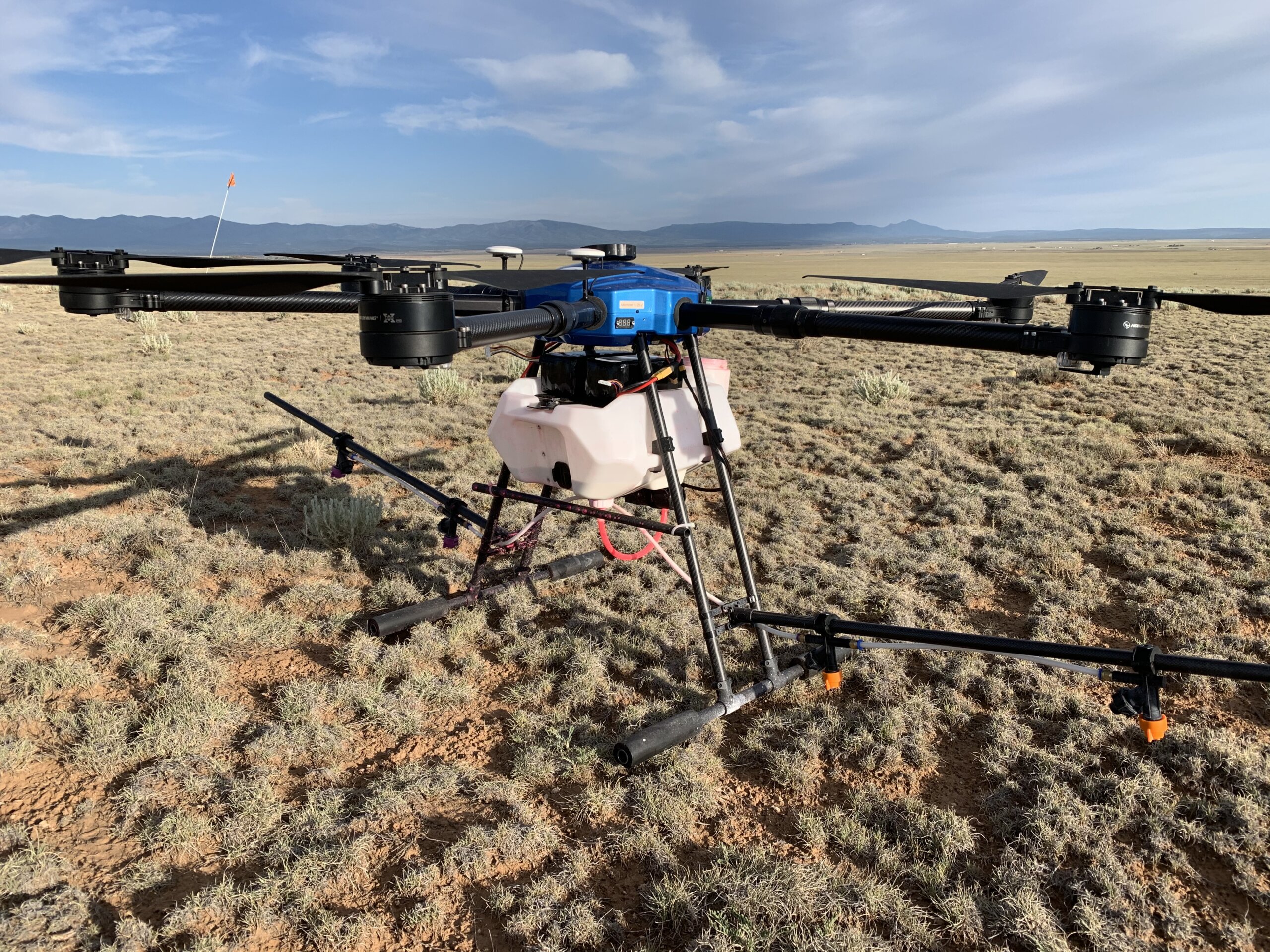
The RPAS was a six-rotor Precision Vision 35 (Leading Edge Aerial Technologies, New Smyrna Beach, FL, USA) equipped with four Turbo TeeJet XR110-01 nozzles (two on each side of the aircraft) mounted to spray booms.
Swathing
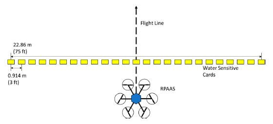
Twenty-six water sensitive papers were placed in a line perpendicular to the flight path, approximately 0.91 m (3 ft) apart, to capture the spray deposition. The RPAAS was flown at a speed of 8.94 m/s (20 mph).
Layout of water sensitive cards and flight line during spray deposition measurements.
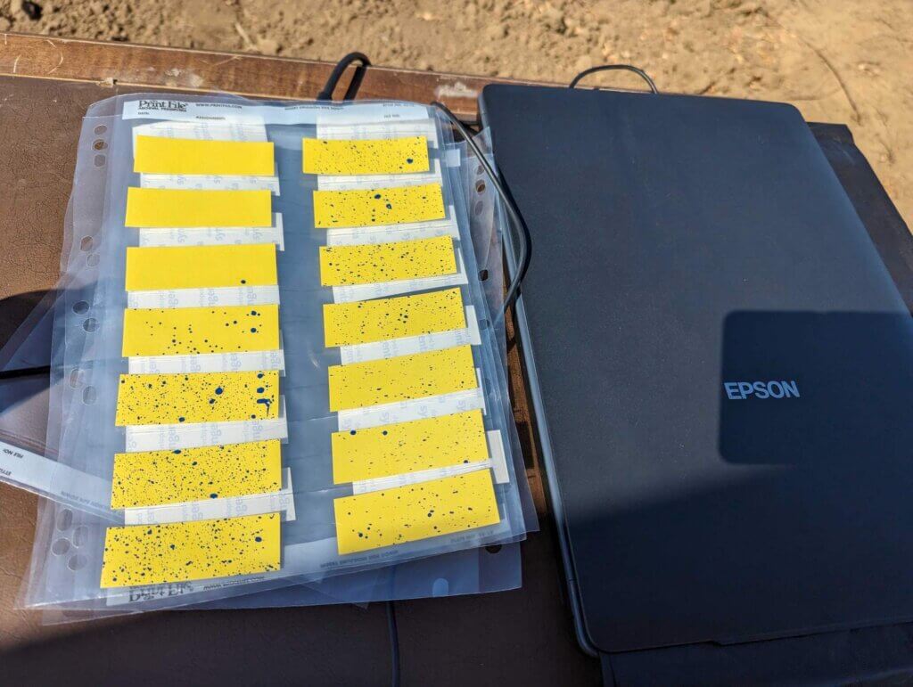
The papers were scanned with an Epson Perfection 1240U laser bed scanner and swath analysis was performed using DropletScan (WRK of Arkansas, Lonoke, AR, USA; WRK of Oklahoma, Stillwater, OK, USA; and Devore Systems, Inc. Manhattan, KS, USA). Papers were scanned at 600 dpi and the software was used to determine the coefficient of variation (CV) for both a simulated racetrack and a back-and-forth spray pattern.
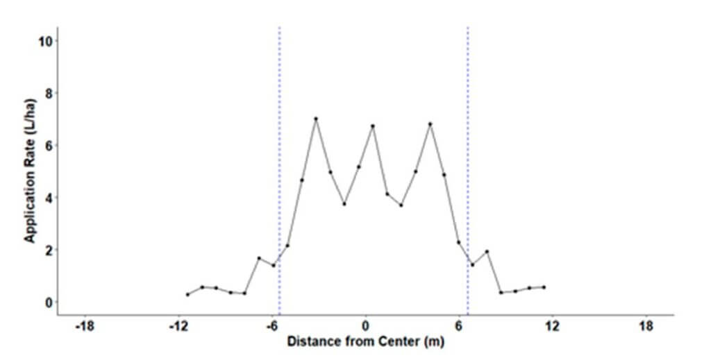
The CV for multiple effective swaths was calculated and the swath width with the lowest CV was chosen for the study. This effective swath width was 12.2 m (40 ft) with an average application rate of 2.75 L/ha (37.6 fl. oz./acre). Following a 50% RAAT IPM strategy, a 24.4 m (80 ft) swath was used for treatments, with an average treated swath application rate of 1.4 L/ha (18.8 fl. oz./acre).
Application rate of tank mixture S across swath. Dashed blue lines indicate effective swath width.
Treatment and Efficacy
Two types of grasshopper population density estimation methods (visual estimation and sweep netting) were performed on the day before treatment (pre-count) and 3, 7, 10, and 14 days after treatment.
The RPAS was flown at 9.8 m/s (22 mph) at an altitude of 3.05 m (10 ft). Treatments with the liquid insecticide Sevin XLR PLUS required a single flight to cover each replicated plot, without completely depleting the battery, and each of the four treatments was completed within approximately five minutes of the total flight time.
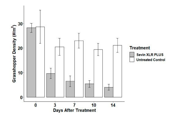
Our results demonstrated that Sevin XLR PLUS significantly suppressed grasshopper populations over a 14-day period (normalized population reduction was 79.1 ± 8.4% SEM) and quite rapidly (mostly by day 3) compared to untreated controls. These results are comparable to those achieved with fixed-wing aircraft.
Effects of Sevin XLR PLUS treatment on grasshopper density and mean ± SEM across the trial period.
Observations
Because RPAS are relatively portable, the potential exists to shorten the average length of time between the identification of a hotspot and a treatment. The RPAS covered the whole test area in a single flight in approximately 5 minutes, making these population hotspot treatment applications relatively rapid, potentially more cost-effective, and more targeted in comparison to fixed-wing aircraft.
We would describe the observed efficacy as successful in the sense that grasshopper populations, when accounting for reduction in untreated control plots, were reduced by 79.1 ± 8.35% SEM. This is very close to what is typically expected for APHIS program treatments, which is 80 to 95% population reduction. Our lower-end results can probably be attributed to the arid conditions, lower levels of rangeland forage observed during the study in that region of New Mexico, and a mobile, rapidly aging population.
Before adoption as an application method option, further research is recommended on using an RPAS to cover larger areas in combination with using diflubenzuron-based insecticides, which are often preferred.
This research was funded by an interagency agreement with USDA-APHIS-Plant Protection and Quarantine (PPQ): 20-8130-0893. It may not necessarily express APHIS’s views.