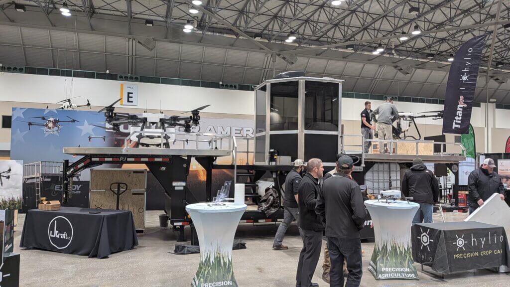
Much of this article is based on a session and tradeshow I attended at the 2026 Drone End-User Conference in Kansas City. I want to acknowledge the insightful information provided by the three session speakers, as well as the ~200 audience members that asked honest questions and shared their experiences. The speakers were Mr. Chase Plumer (Owner, ProBuilt Fabrication/ProDrone Spraying & Seeding, Seymour, IN), Mr. Klaytin Hunsinger (Owner, Hunsinger Ag Solutions, Rossville, IL) and Mr. Kyle Albertson (Owner, Albertson Drone Service LLC, Benton County IN).
Tendering systems
Drone-based crop protection is a rapidly growing industry and operator experience spans from novice to veteran. It follows that tendering systems are not a one-size-fits-all proposition. The best fit will be a configuration that is budget-conscious, reflects the size and nature of the operation, and accounts for future needs.
We can categorize them by their complexity, cost and capacity.
Entry-level tendering system: A starting point
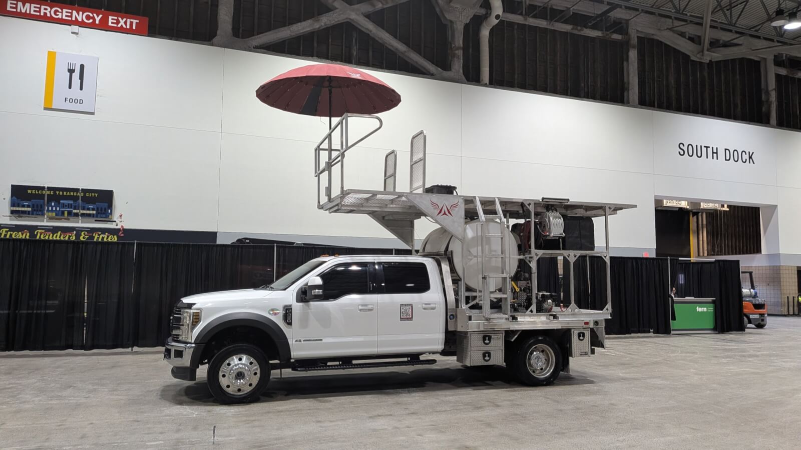
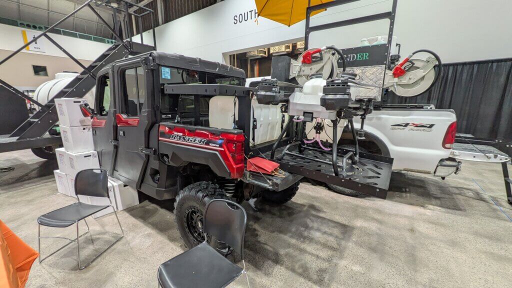
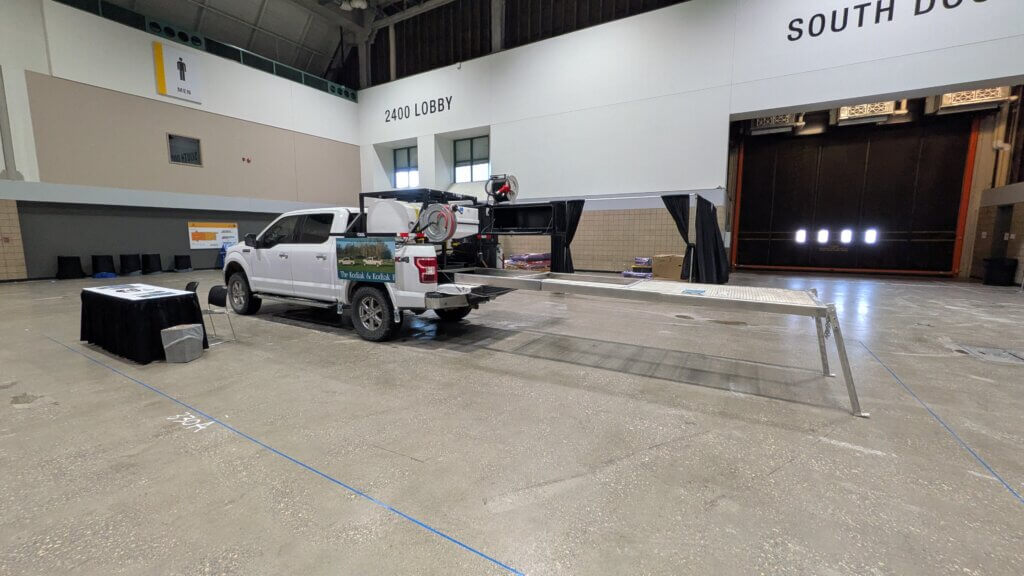
For those just getting started, focus on affordability (lower initial investment) and simplicity (basic components). Examples include skid or truck builds, which are removeable or permanent systems that either rest on a vehicle bed or are built on-and-around the vehicle. This is an operator-friendly system that is small and portable for easy access to diverse fields. It’s the least durable configuration, and not particularly efficient or upgradeable, but it will serve until you know what you really need and how you like to work.
Mid-level tender system: Second year
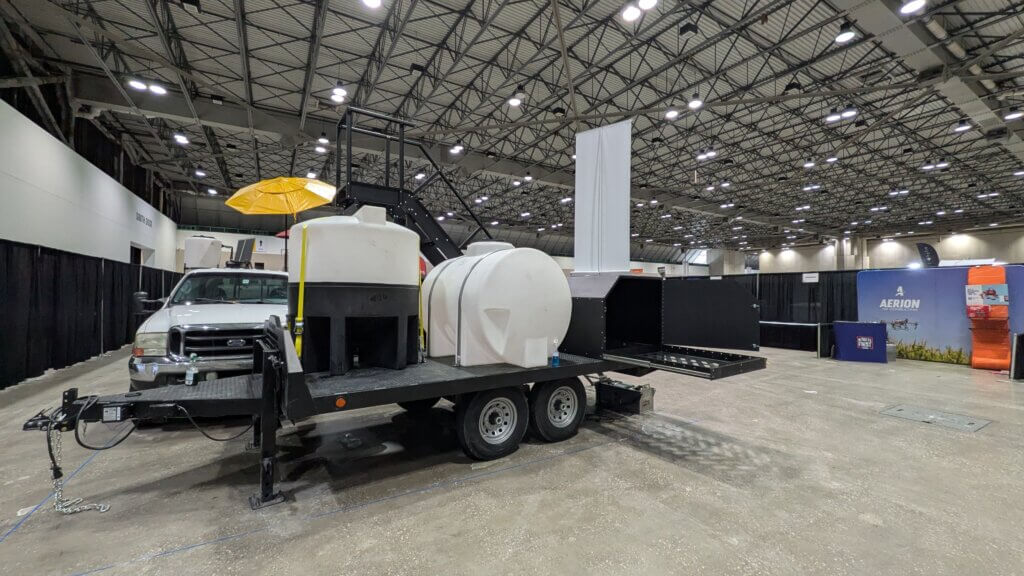
By year two, you might want a larger and more efficient configuration with additional storage and a few creature comforts to reduce operator fatigue. A truck build might suit, but this is more likely a trailed system that is still capable of being towed by a mid-sized (1/2 to 3/4 tonne) truck. Some operators feel enclosing the trailer reduces efficiency, while others appreciate the security and protection afforded by defined spaces.
A mid level system has some capacity for modification, but isn’t designed to support multiple drones, and likely won’t have enough capacity to store a day’s worth of water, chemical, or fuel. The operator may wish to detach the truck to run for supplies. Or perhaps it makes more sense to run a truck with a skid-mounted tender system that trails a second, mid-level system to divide-and-conquer, or scale up for larger projects.
Beware going too big, too quickly. A 30-foot gooseneck can get caught on hilly terrain, where a 20-foot flat bed with a straight truck might be better suited. Small to mid-size trailers also take less time to set up and tear down. Consider performing site recon before dispatching a mid-level tender system. This is an additional step, but it allows the operator to scope out potential hazards and is ultimately more productive because it prevents tender systems getting stuck or placed in inefficient or unsafe locations. For example, if a client is “plant-out, pick-in”, the fields are hard to service because there’s no way to access them with large vehicles. Pilots become landscapers, spending valuable time clearing an operations area.
High-level tender system: Large scale and Commercial interests
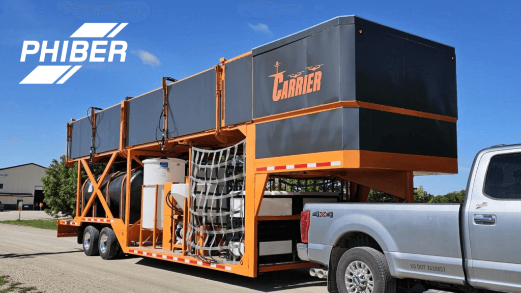
Made for efficiency, the limiting factor of this system is the drone’s productivity. This category is comprised of the largest gooseneck trailers, which may include an upper deck and enclosed areas. It has the highest capacity for water storage, can service multiple drones and has ample storage. Intended for large fields, the size of this unit can make it physically incapable of reaching smaller fields. While a one tonne truck might be able to tow it, an even larger vehicle might be more suitable. It may also be prohibitively inefficient given the time required for setup and teardown. Consider an operator that requires a 15 minute start-up and a 15 minute teardown to spray 250 acres at 50 ac/hr; At $20/ac, that’s roughly $500.00.
Components
Fundamentally, each tendering system has the same function, so they share the same basic components. Here’s an overview of common features and considerations.
Trailer
The trailer is (literally) the foundation of most tendering systems. Operators suggest building for your current budget but planning for future needs as best you can. Trailer size should reflect the nature of the farms you will be servicing and how best to access them. You should also consider the safest and most efficient workflow on and around the trailer before committing to a layout.
Option 1 – Utility trailer
| Advantages | Disadvantages |
| Easy to get on/off | Low ground clearance |
| Less expensive | Narrow footprint for accessories (e.g. conventional tanks not fitting between wheel wells) |
| Versatile (use for drones on season, and other tasks off season) | Narrow if planning a top flight deck |
| May be an insufficient trailer GVWR (Gross Vehicle Weight Rating). This is the maximum allowable total weight of a trailer when fully loaded. |
Option 2 – Flatbed gooseneck trailer
| Advantages | Disadvantages |
| More room for accessories | Much heavier. ¾ tonne truck likely not sufficient. |
| Better ground clearance | Hard to get into tight places (length dependent). |
| Higher GVWR | Set up / Tear down takes longer |
| Potential for top flight deck. Typically, 102” wide, so top deck can be about the same. |
Option 3 – Enclosed trailer
| Advantages | Disadvantages |
| Protection from weather and elements | Limited clearance for large drones (e.g. 24’ long, 8.5’ wide) |
| Increased security for equipment | Highest GVWR |
| Could serve as mobile workspace / office | Most expensive |
| Cleaner environment for charging batteries, and generators don’t need maintenance (e.g. filters changed) as often. | Can get hot inside, both for people and battery overheating. Airflow on batteries is a necessity, and fans can only cool to ambient. Drone hasn’t got time to cool between fields. |
Vehicle
Based on operator discussion, it seems many have a tendency to push their trucks to the limit… or beyond it. One operator uses a ¾ tonne truck to pull a 22-foot trailer with an upper deck. Another uses a 1 tonne (aka tonner) gas F350 which struggles to pull a 30-foot trailer. Others recommended the use of a single axle semi (e.g. a Kodiac or a Kenworth T300), which even used still has ample life left in it, and at ~15 to 17,000.00 USD is cheaper than buying a truck.
Consider that if you run a two-person operation, you may want more than one vehicle. A smaller truck can be employed to run for parts or fuel, or as previously noted can be fitted with a skid mount and a 1,300 gal. poly tank to split up the duty.
Tanks
Tank size(s) will depend on how you choose to operate, how many acres you plan to do in a day, and the weight capacity of your truck and trailer. Again, there is no one solution, so consider the following scenarios before you commit.
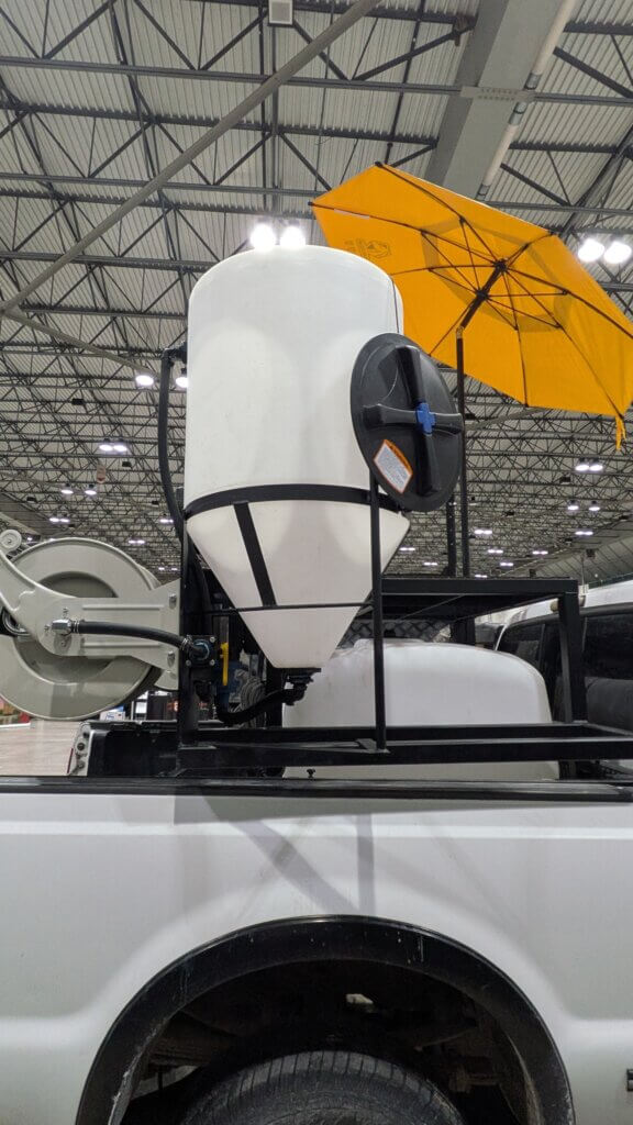
If you plan to hot load, perhaps you’ll just mix in a single, large tank. However, if you plan to switch between insecticides, fungicides and herbicides, one or two 100-gallon cone-bottom tanks with wash-down nozzles might make more sense. Then, you can carry clean water separately in a few repurposed IBC’s or go for the efficiency of a single, high-volume poly or stainless tank. Consider the most flexible and efficient arrangement.
Will you have access to water, will you have water tendered, or will you carry enough for the day? Will you fill from a 3-inch connector or suffer the lost time and fill with a garden hose? Will your truck and your trailer handle that weight, and will the vessel(s) fit between the wheel wells? Are the tanks black or shaded to prevent algae and do you have a plan to baffle the volume, so it doesn’t slosh when you drive over uneven terrain? Larger poly tanks (e.g. ~1,000-gallon tanks) have spots molded in to accept baffles, but some operators noted it’s difficult to install them after-market. Slosh suppressors such as floating balls or lengths of poly French drain can help.
Pumps and Lines
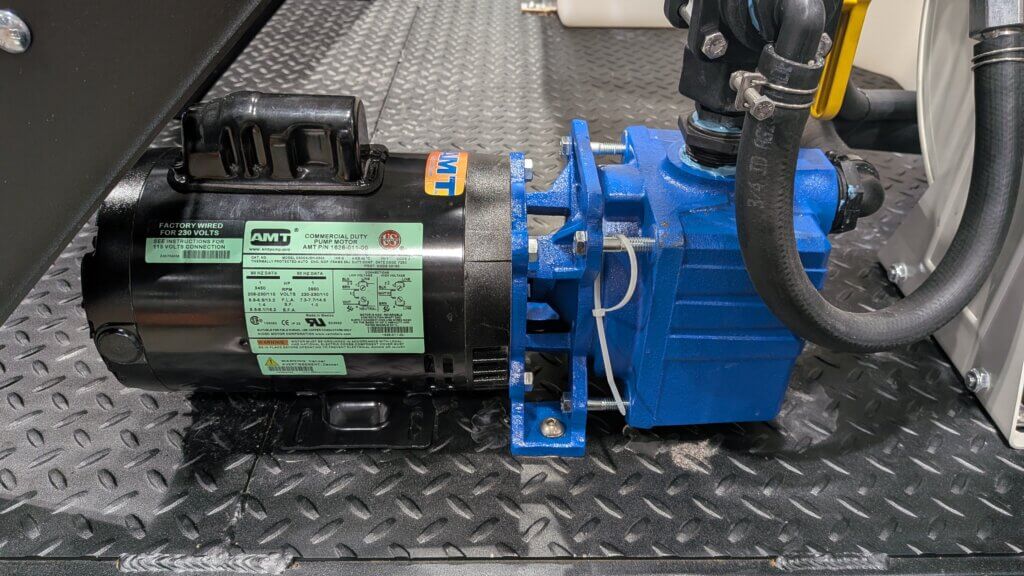
While some prefab trailers offer pneumatic pumps, most must choose between electric and gas pumps, and there are pros and cons to both.
| Electric Pump | Gas Pump |
| Low noise | High noise |
| No exhaust | Exhaust |
| Taxes the generator | Does not tax the generator |
| No fuel | Requires fuel |
| Low maintenance | Regular maintance |
| May limit head pressure | Ample head pressure |
Gas-powered pumps (e.g. Drummond or Predator transfer pumps) are relatively cheap, but some claim they have a high failure rate. This not only incurs downtime, but operators must deal with the chemical in the pump and lines during repair.
Electric may be a better choice, if only to avoid the noise and exhaust, and some operators run them continuously to recirculate chemistry when not filling a drone. Consider the horsepower, gallons per hour and head pressure, especially if you are pushing flow to an upper flight deck.
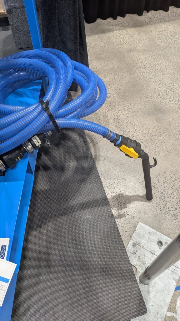
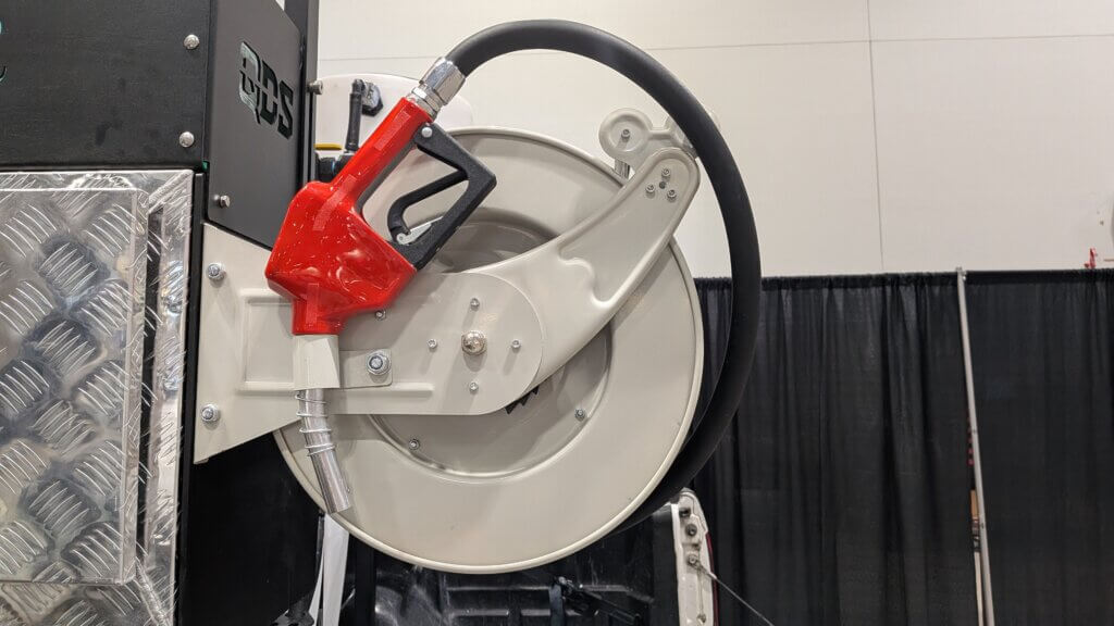
You should be able to fill a drone in about a minute. Some operators have begun increasing fill line diameter from 1-inch to 1.5-inch but feel 2-inch lines are too heavy to warrant the few seconds saved during filling. This may not be a limitation, however, if they are part of a top flight deck arrangement, and not dragged along the ground.
The auto shutoff function of a fuel-pump-style filler is preferred over a quarter-turn-style. The former contributes to foaming but some operators say that can be mitigated by using an anti-foam adjuvant and it’s less likely to create an overflow situation.
Perhaps a metered flow valve that shuts off once a predesignated volume has been dispensed would be a workable solution. This would preserve speed, but without foaming or potential overflows.
Generator
This proved to be a controversial subject at the conference. Many operators were unwilling to promote a single make or model, but the discussion resulted in some general guidance based on personal experiences. Generators will have a peak and a continuous performance rating. Ensure the sum total of all your draws does net exceed the continuous rating.
Drones are getting bigger, and the number of electrically powered devices on the trailer is increasing. Smaller operations tend to employ mobile gas generators that produce less than 10 kW. Larger operations reported using 30 kW (or more) diesel standby generators to charge two drones, plus accessories, while ensuring room for future growth.
A mobile gas generator (inverter or not) tends to be the cheaper, lighter alternative, depending on the wattage. They are a good choice for entry level systems and with regular maintenance will last longer, but are still a short-term proposition. Diesel generators tend to be more expensive, but are quieter, more fuel efficient and more reliable. A liquid propane standby generator is yet another option; Generally cheaper than diesel, consideration must be given to the weight and size of what is typically a 250-gallon propane tank.
A few points raised by operators during the discussion:
- Most standby generators do not need diesel emission fluid, while mobile generators do.
- Many operators prefer the durability of mobile generators over standby generators. The former is built to be moved while the later presents issues with brackets, mounts and stators.
- Warranties are advisable for inversion generators, as they are not easily repaired.
- Standby gas generators (10 kW continuous / 13 kW surge) may require you to downrate the battery charger, or the heat can trip the breakers. It is not advisable to bypass breakers.
Storage
Storage is often overlooked but can be critical to efficiency. For example, if you plan to spray six, 50-acre farms in a day and it takes 10 minutes for set up and 10 for tear down, that’s two hours gone. Consider what you’ll need and where you’ll need it, and place storage accordingly to minimize downtime. PPE should be located near your flight deck or filling area. You’ll also want to consider carrying spare parts, such as an electronic speed controller, motor, pump and a full set or rotors.
Batteries
Some battery chargers feature water baths, misters or air conditioning, but at bare minimum batteries should charge in the shade and in a ventilated area (e.g. not enclosed in a storage or tool box). One operator vented air from a commercial blower fan to the batteries on the top flight deck.
Connectivity
A hotspot on your cellphone doesn’t always provide reliable service. Satellite internet providers such as Starlink or Xplore (depending on your location) might be a solution. If the controller drops a direct signal to drone, it can bridge to satellite to connect to the SIM card in most drones. Operators that use this system advise it’s best to rent the hardware (if possible) so if something damages it, you get a free replacement. 100 gb of monthly roaming has proven more than enough for most operators.
Mounting solutions vary, but operators noted good experiences with companies such as Veritas Vans, which have a replacement policy. They warn against 3D printed options that tend to be produced using unsuitable filament materials. Operators that use magnetic mounts on their trucks have reported no issues. Some run wire through rear window or sliding door, and others pull the headliner down and run the power cord out through the third brake light.
Operator safety
Lastly but certainly not least, when it comes to the cost-benefit assessment of tender features, safety should always be a priority. Even simple comforts such as folding chairs combat operator fatigue, increase safety and happily also improve overall productivity. We’re none of us getting any younger.
RV awnings, umbrellas, foldable Bimini-style tops or flip-up doors provide shade. Switching to lower-decibel equipment (e.g. inverter gas generators run at about 90 decibels and electric pumps are even quieter), enclosing loud systems, or positioning them far from the filling area, reduce noise and emission exposure. Chemical drift and exposure during filling should be considered, and PPE should be used and stored in convenient locations.
Trailers that feature an upper flight deck sometimes include a central cable to tether belt harnesses. Stationary railings can help prevent falls, while a fold-up version provides clearance when backing the trailer into a shed.
The drones themselves are a hazard. Long flight decks keep landings and lift-offs at a safe distance, and a protected cockpit area improves matters. Decks with pull-out platforms or hydraulic wings can increase the operating area and can be adjusted to account for adjacent roads and the slope of the ground. A short rail around the landing area can prevent a drone from slipping off; A falling drone is expensive, but falling or sliding into an operator is a disaster. The simplest approach might be to operate on the ground.
Take home
The speakers left the session with some summary advice.
- Trailer first, equipment second.
- Build for today and tomorrow.
- Function over form (stability, balance and access over appearance, bearing in mind that if it is a business, it can’t look terrible, either).
- Efficiency from day one. Run a stopwatch (when the crew isn’t watching). Find and change the limiting factor, if it’s changeable. The right trailer improves efficiency even before the first acre is sprayed.
Thanks to the many speakers, attendees and trades people that contributed to this article. If you want to share pictures and specs for your tender system, let us know! If we get enough interest we’ll publish an article showcasing your tender systems so others can learn from your experience.


