Article reprinted with kind permission from an original article written by Oliver Hill in the February, 2017 edition of Farmers Weekly. Photos ©Kathy Horniblow.
Crop spraying is one of the most important and highly skilled jobs undertaken on any arable farm, but it is facing increased public scrutiny. This is why it is vital that the kit you use as a means to apply pesticide to crops is in prime working order and is set up correctly to deliver the product safely and accurately to its target. Optimum sprayer set up will help to maximize the efficacy of applied products, reduce spray drift and keep machinery in good condition.
For this best practice guide to sprayer set up, Farmers Weekly teamed up with former Farm Sprayer Operator of the Year Iain Robertson. Mr. Robertson is assistant arable farm manager at David Foot Ltd, a 2,200ha mixed farm south of Dorchester in Dorset, growing wheat, barley, beans, oilseed rape and maize as forage for the farm’s three dairy herds. The machine used for this guide is a Bateman RB26 self-propelled sprayer and while most of these checks and tests are universally applicable to all sprayers, it is also important to refer to the handbook of the manufacturer of your specific machine.
Watch the video tutorial with Mr. Robertson and then see the step-by-step guide below for more detail.
Pre Start Checks
Before firing up the engine, the first thing to do is your pre-start checks – that means checking your machine’s vital fluids like fuel, hydraulic oil, hydrostatic oil, engine oil and coolant levels. If yours is a self-propelled sprayer, chances are you’ll need to get up on to the back of the machine to check some of these.

“While I’m up on the back of the sprayer I also have a quick look in the top of the tank to make sure that it is nice and clean and the tank rinse nozzles have worked properly – cleanliness is next to godliness,” says Mr. Robertson. Next, move on to the tires. Use a pressure gauge to check all tires are at the correct pressure and refer to the manufacturer’s guidelines. If you’ve got a trailed sprayer, don’t forget to check the tractor tire pressures as well.

Aim for tires to be run at the lowest pressure recommended for the load to be carried. This will help with boom height and stability and also helps tires act like a shock absorber to ride out bumps. If using a trailed sprayer, use a spirit level to ensure that the drawbar is level. Mr. Robertson says he tries to work around the machine in a methodical, clockwise manner to ensure that he doesn’t miss anything.

Coming to the pumps, check that they have got enough oil, check that any tool boxes have enough spare parts and any equipment needed and make sure you are carrying a spill kit with absorbent granules and a spade in case the worst happens and there is a spillage. Make sure all parts are lubricated daily and that any grease nipples are cleaned before and after use to avoid them collecting dirt and blocking.

Check all hydraulic hoses, spray lines and air lines for any signs of wear that could result in problems while operating.

It’s best to run the sprayer at a minimum of 5 bar to check for leaks. Also check the spray tank is fixed down securely, all straps and bolts are tight.
Boom checks
Once opened out, check the boom has good movement in the x- and y-axis. All machines are different so check with your manufacturer as to how the boom is set up. Mr Robertson’s Bateman has tie rods and stock bots that can be adjusted to set the boom up to ride well.

Check the tie rod nearest the back of the machine is slightly loose when moving and that the front rod is tight. Next, check for up and down movement by gently pushing the boom down by about 50cm and letting go. The boom should return to the central position without too much bouncing around.

“We want a little bit of movement but not excessive so that you can ride over the bumps as you go along without over- and under-dosing the crop,” says Mr. Robertson. Boom height is one of the most critical factors when spraying and the ideal height is 50cm above the crop. One of the easiest ways to work this out is by using a cable tie that is cut off at the correct length to use a visual aid from the sprayer cab.
Don’t forget to measure from the tip of the nozzle to the crop, not the spray line.

Good sprayer cleanliness is important, so make sure the system is rinsed through at the end of each day with clean water to make sure there’s no residue left in the boom. If your machine’s boom doesn’t have recirculation, remember to take the end caps off occasionally and flush out the whole boom.
Nozzle checks
Check that the nozzles are aligned both vertically and horizontally, according to the NSTS guidelines. Loosen clamps to adjust any nozzles that need realignment.

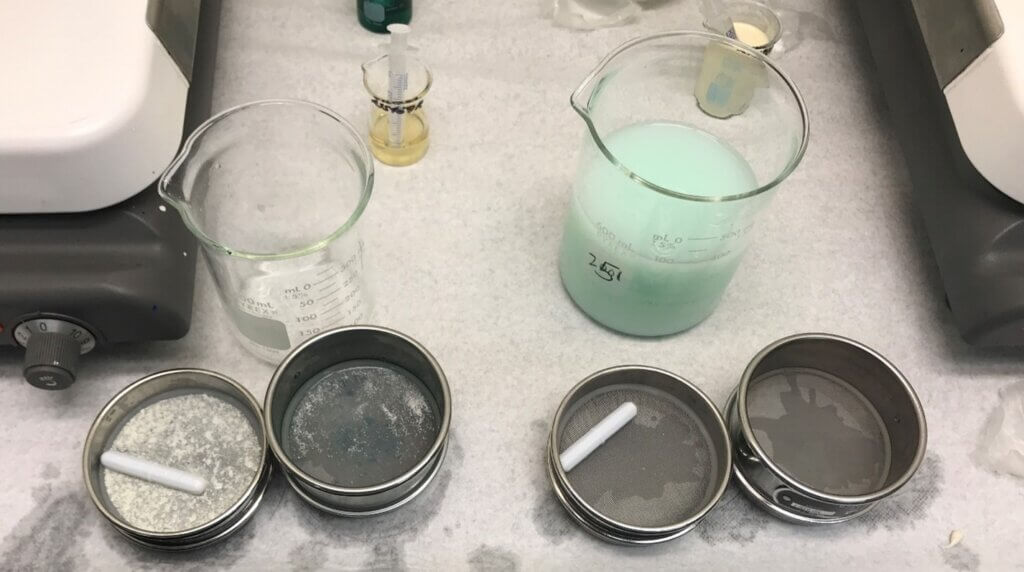
Check the nozzle output at least twice a year by running the sprayer with clean water at 3 bar pressure. Time the output of each nozzle for 30 seconds. If nozzles have been used previously, it’s best to check their output against that of a new pair. Mr Robertson advises using a measuring cylinder rather than a jug to measure the flow rate as a jug is less accurate “because you get a bigger variation over the wider surface area”.

With an 03 nozzle running for one minute at 3 bar pressure, the output should be 1.2 litres/minute as a rule of thumb but refer to the nozzle manufacturer’s output chart for the expected flow rate. “An easy way to remember this is: at 3 bar your nozzle size multiplied by four will give you your target litres/minute output. It works for all nozzle sizes.” If the output varies more than 4% of the average, or if the spray pattern visually doesn’t look correct, you need to change the nozzle set.

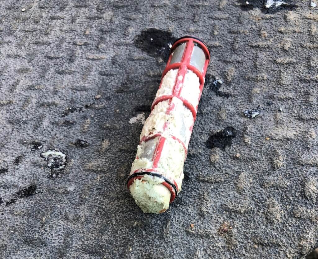
After checking the output, cross-reference this figure with the rate controller – you may need to adjust the flow figures to ensure that the two correlate. If a nozzle becomes blocked while spraying, Mr. Robertson says he will swap it for a new one and then clean it later using a toothbrush or airline. Never blow through a nozzle with your mouth.

Nozzle choice
The choice of nozzle is highly dependent on the sort of job you’re doing. “Timing is crucial but using the right nozzle at the right time will make the job so much easier, cut drift and mean that you’re getting more of the product where you want it to go. If you aim at it you will hit it,” says Mr. Robertson.

His nozzle of choice is an 03 size and he prefers to use the Defy 3D nozzle alternated forwards and backwards across the boom for pre-emergence work and T0 applications as well as the T3 ear spray. “In less than optimum conditions I may prefer to use the Amistar/Guardian Air, a fine induction nozzle. I would use this at T1 and T2 and also in sub-optimum conditions.” This nozzle has a 3-star Local Environmental Risk Assessment for Pesticides (LERAP) rating and is 75% drift reducing.
A water volume of 100 litres/ha is a good rate for spring fungicide application. It provides enough coverage for good disease control and allows maximum efficiency from the sprayer.
Forward speed
The third and final part of reducing spray drift is forward speed. Depending on nozzle size and water volume, aim to travel at 12kph.

Mr Robertson says he finds that this speed gives a good overall output and means you don’t get shadowing or turbulence behind the machine.
Tips and tricks
One of the biggest risk of contamination is at fill up. “A fantastic, cheap trick that I learned through Farm Sprayer Operator of the Year is to take a 200 litre plastic drum and cut it in half to create two drip trays to catch any spillages under the induction hopper and the tank overfill.” This eliminates point source contamination, he says.

“Finally, there’s a plethora of information out there on the internet, loads of good apps to download. The technology is there to help us do the best job possible and make our job as safe as possible.”