The Hypothesis
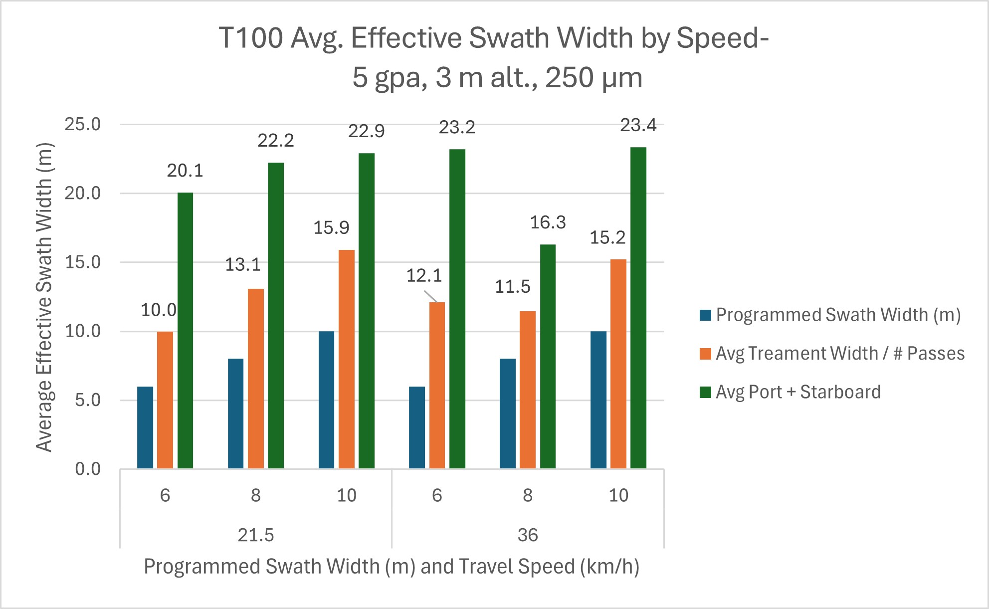
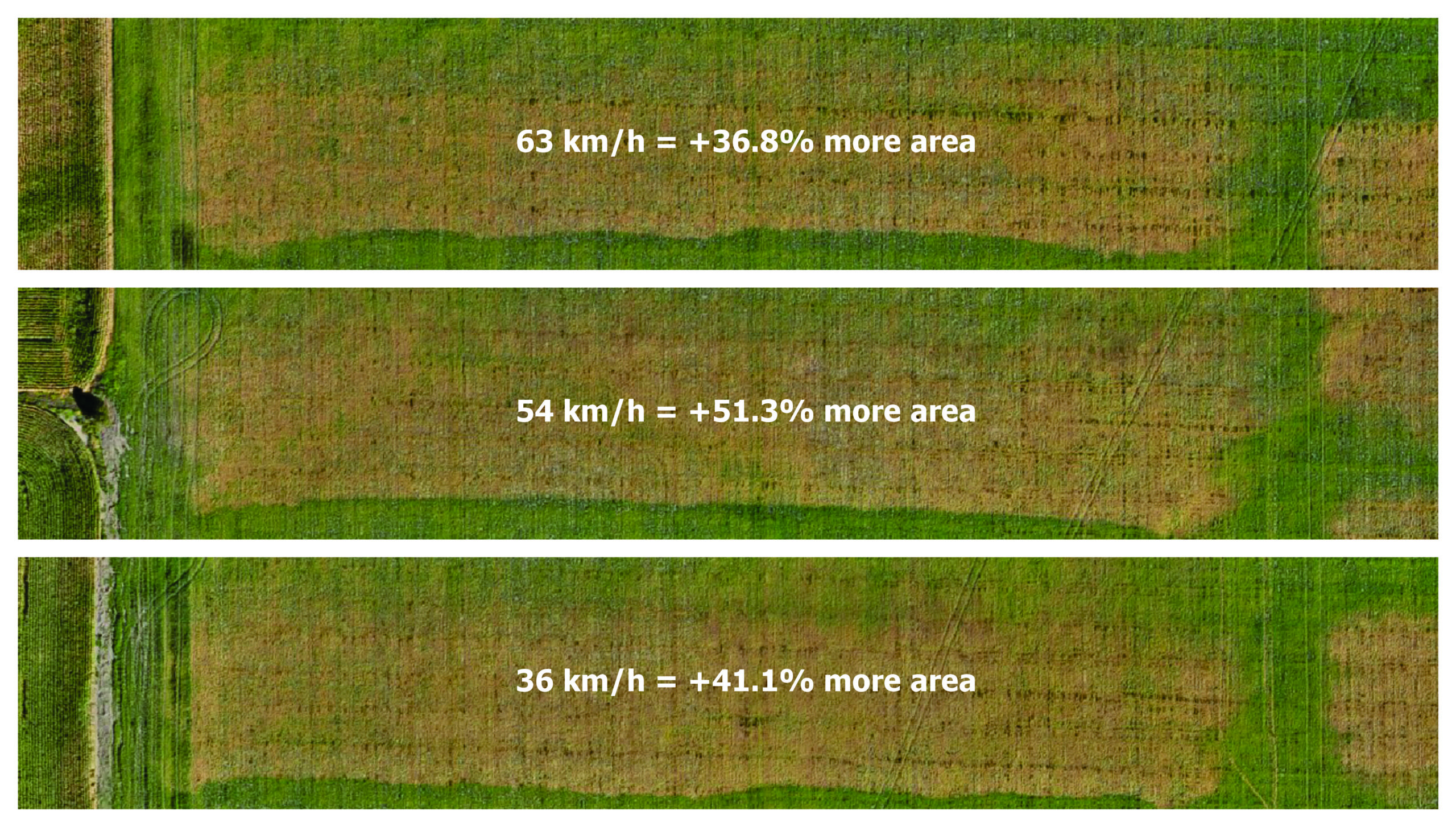
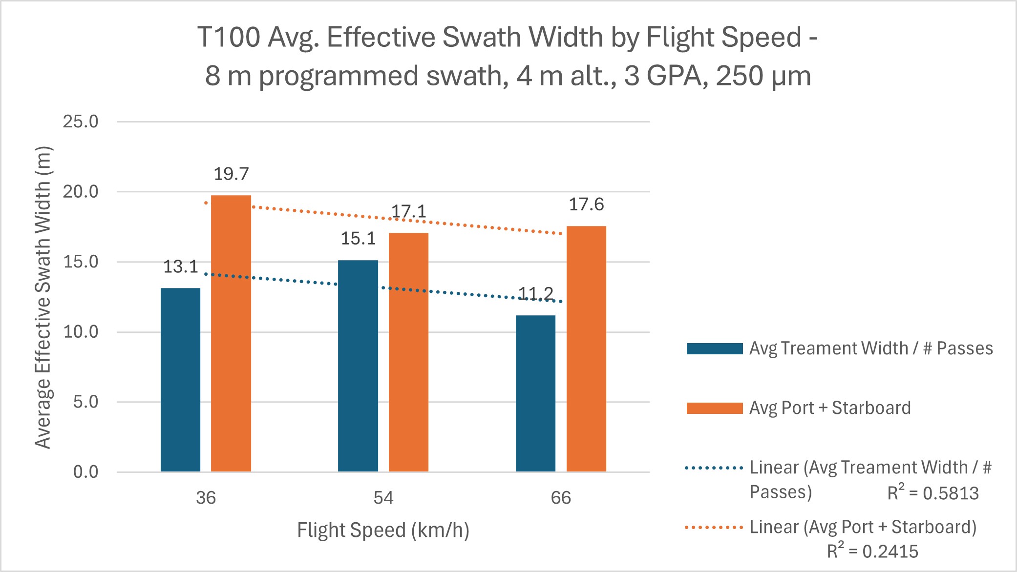
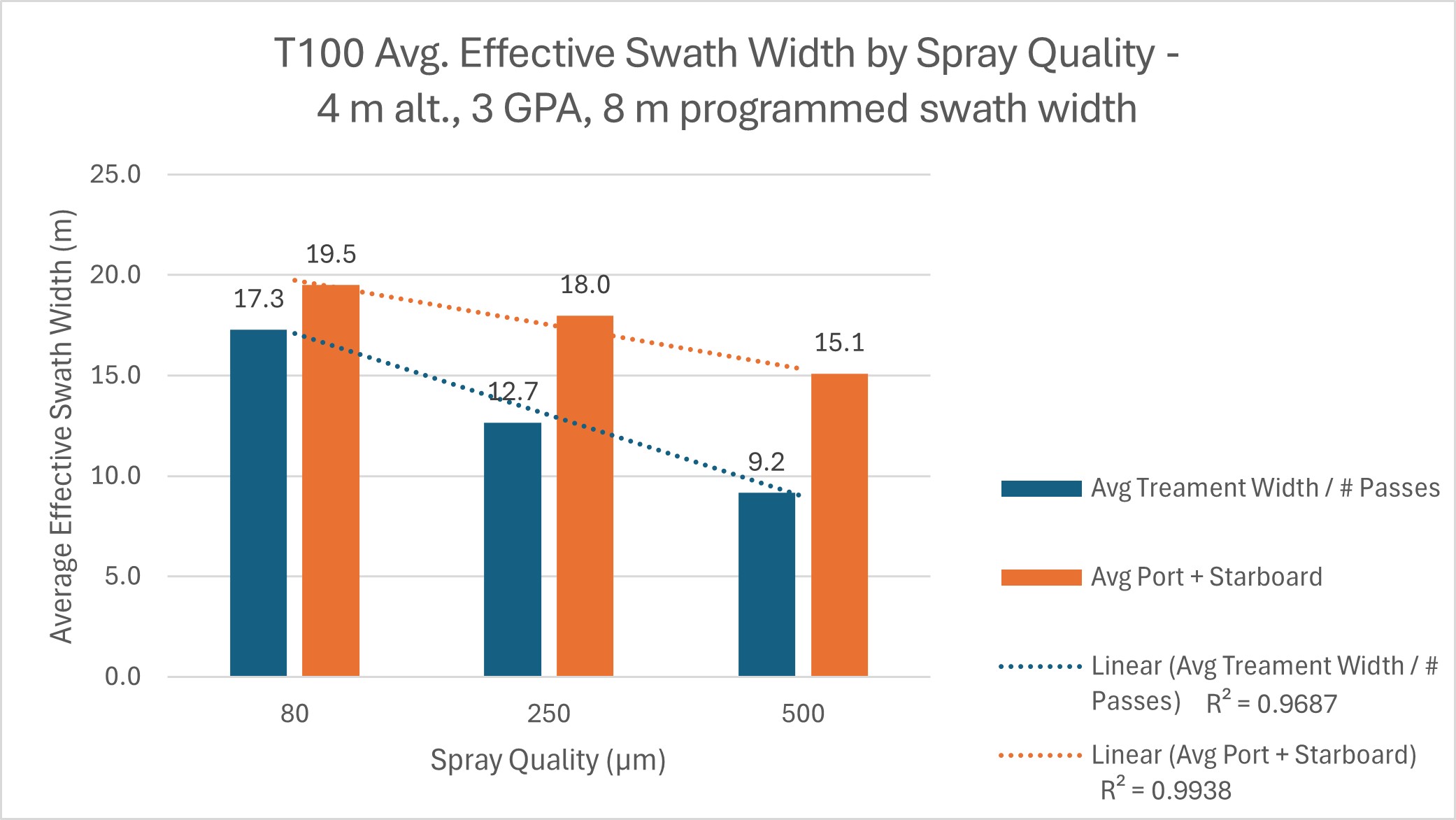
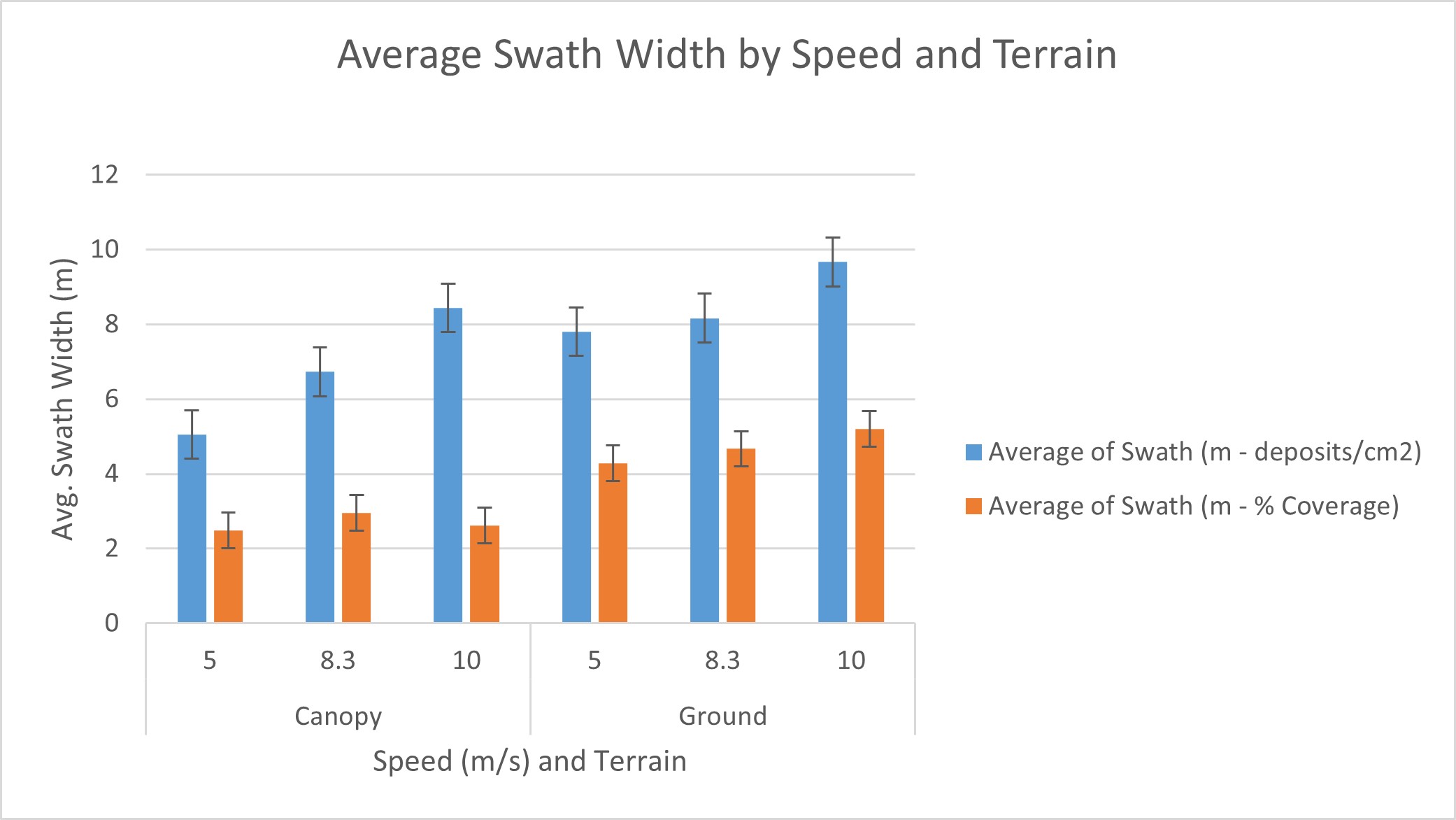
The results of a recent herbicide deposition study performed with the DJI T100 led us to observe that after ~13 m/s, swath width and drift were no longer directly related to travel speed; They appeared unaffected. The result was completely unexpected as it was counter to several years of prior study with smaller drones. This led to a hypothesis that the aerodynamics of this new generation of quadcopters might be similar to that of a helicopter, and it was impacting spray deposition in a similar fashion.
Let’s use the stages of quadcopter flight to set up the premise.
1. Hover
When a drone hovers, each rotor draws air from above and accelerates it downward in a high-velocity blast. The cumulative effect is a vertical component referred to as the “downwash” and the turbulent splash of air that hits the ground and spreads laterally is the “outwash”.
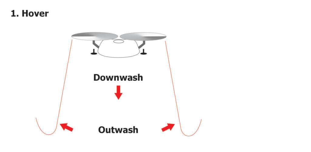
The initial strength of the downwash depends on the degree of “disc loading” which is the weight of the drone divided by the rotor area. The intensity of the downwash wanes with distance from the rotor, spreading out in three dimensions until it impacts the ground and becomes the outwash.
During hover, the drone recycles some of its downwash. This turbulence affects the stability of the drone, requiring a great deal of power to stay aloft, especially when it’s full.
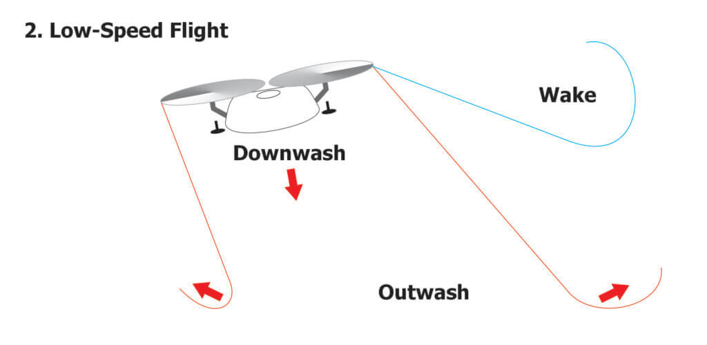
2. Low-speed flight
A helicopter achieves forward thrust by changing the pitch of its rotor blades. Most drones have fixed-pitch rotors, so the entire drone must tilt forward to enter low-speed flight. This causes the column of downwash to tilt backward.
While the downwash is created by lift, “wake turbulence” is created at the tips of the rotors as high-pressure air beneath the rotor wraps around to the low-pressure area above. As the drone flies at low speed (~<3 m/s) the wake is visualized by a pair of counter-rotating, cylindrical vortices that trail behind. Some journal articles suggest the downwash for medium-sized drones (e.g. < 50 L capacity) detach from the ground at speeds as low as 3 m/s.
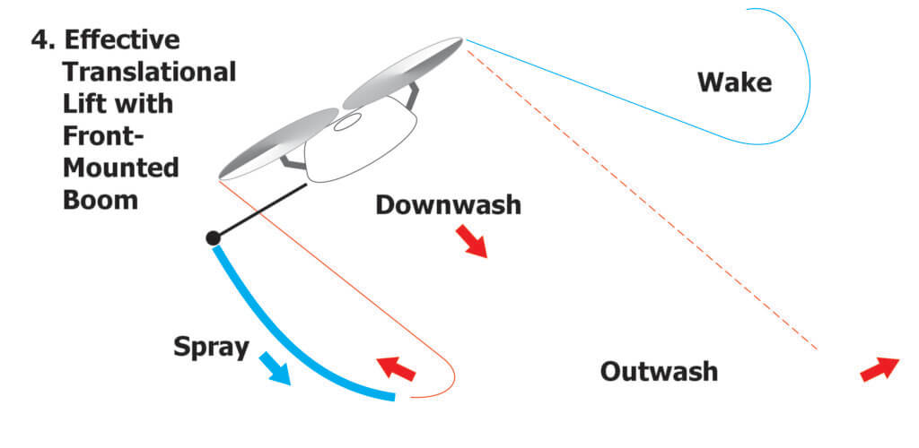
3. Effective Translational Lift (EFT)
As the drone accelerates it continues to angle forward, likely not exceeding 30°. At some point (~15 m/s?), we suggest it enters a state of “effective translational lift”, becoming more stable and therefore more energy efficient. This speed is notably slower than is commonly reported for a helicopter.
During the transition, the drone behaves more like a wing as it essentially outruns its downwash, moving undisturbed air over the rotors. This horizontal air provides some lift, making flight more energy efficient, at least until drag begins to pull on the drone.
The Possible Effect of Flight Stage on Spray Behaviour
Droplets released beneath a drone at hover are completely entrained by the downwash. The majority get driven to the ground and then laterally along the outwash, while some small portion (likely smaller droplets) recirculate back up through the rotors.
At low-speed flight, the downwash begins to tip backwards and the downwash trails behind and at some point detaches from the ground. Spray released beneath the drone is still entrained and will trail on a downward and rearward vector in that downwash. However, a portion will get caught in the wake. We can sometimes see this spray separation occur when lighting conditions are just right.
As speed continues to increase, much of the spray would still be entrained in the downwash, but a greater portion would get caught in the wake, appearing as spray curling at the extremes of the swath. At some point, perhaps if and when the drone enters EFT, the the downwash might be less chaotic and behave more like laminar air. In which case some spray would still curl in the wake, but much of it would fall in a more stable sheet. Further increases in speed would not affect spray behaviour appreciably.
Taking Advantage of ETL
If this is the case, it is conceivable that rotary atomizers positioned under the front rotors could fling some droplets beyond the leading edge of the downwash. What if instead, it were a horizontal boom positioned out in front of the rotors, transecting the chord line?
As the drone tipped forward during high-speed flight, so too would the boom, bringing it closer to the ground and releasing droplets ahead of, and below, the leading edge of the downwash. This should produce a more uniform swath, perhaps subsequently pushed down as the drone passed over.
It’s an interesting idea that is only made possible when drones are capable of high-speed flight.
Reception
In January 2026 I presented this concept during a lecture at the 4th annual Drone End-User meeting in Kansas City. The response was polite, but skeptical. I then shopped the idea around the trade show floor where drone manufacturers suggested a front-mounted boom would interfere with obstacle avoidance sensors, or shift the centre of gravity, making the drone difficult to fly and to land. And what about the impact of wind speed and direction? All good points. Then, Nino Carvalho introduced himself.
The Carvalho Boom
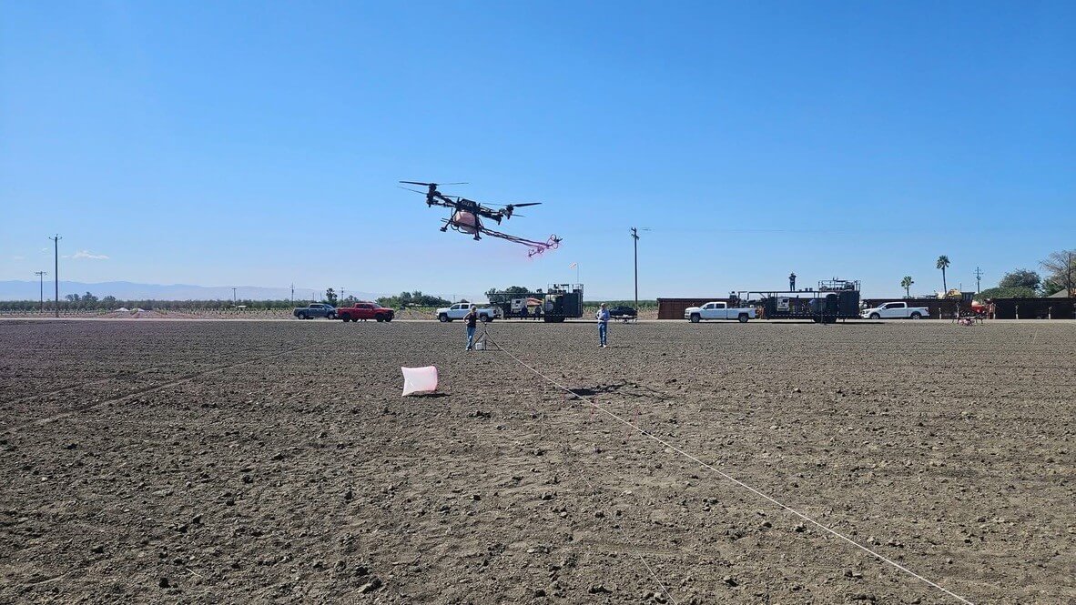
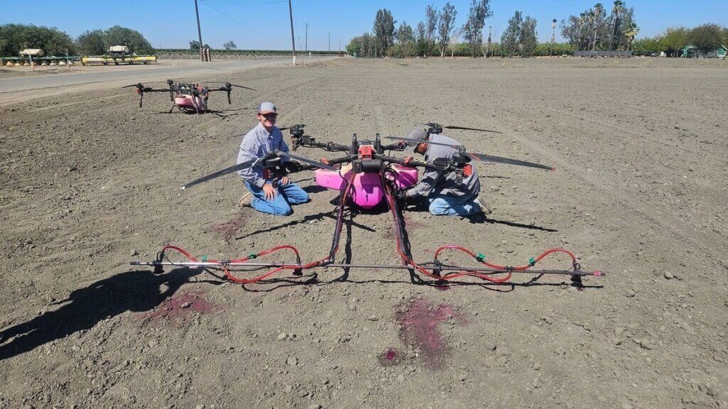
Nino Carvalho and his son, Emilio, own and operate NC Ag Spraying in the Central Valley of California, USA. Emilio was inspired to modify his drone after discussing matters with his mentors; one who owns and operates a fixed wing aerial business, and another that pilots a Huey helicopter. In late 2025, they designed and built a horizontal boom which I’ve dubbed “The Carvalho Boom”.
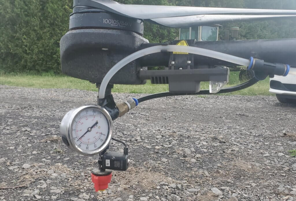
Their first attempt was with a DJI T50, but the boom mount interfered with the stacked rotors, and the atomizer cables were difficult to extend. The XAG P150 had fewer cables and only top-mounted rotors, so it was a better fit. After experimenting with various materials (PVC was too flimsy, steel too heavy) they mounted a length of ½ inch metal conduit directly under the drone.
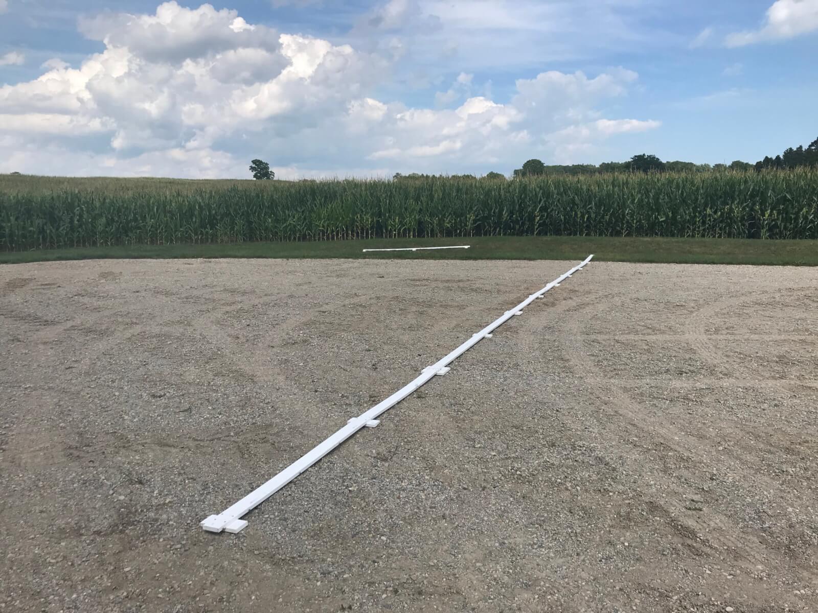
In California, aircraft booms must be limited to 90% of the rotor width (because of rotor tip vortices). The greatest span of the rotors was 312 cm (122.8 in), so they made the boom 275 cm (~9 ft) long. They spaced the rotary atomizers evenly along the boom every 69 cm (~ 2 ft 3 in), extended the original 30.5 cm (12 in) nozzle cables to 305 cm (10 ft) to reach their respective electronic speed controllers, and plumbed them using 1.25 cm (0.5 in) diameter tubing.
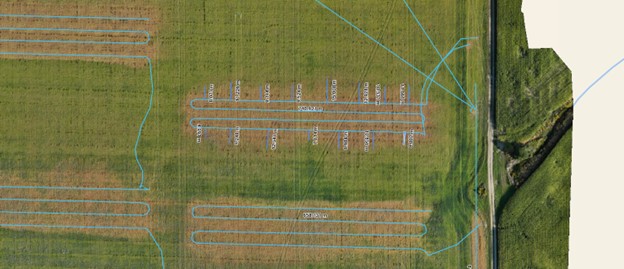
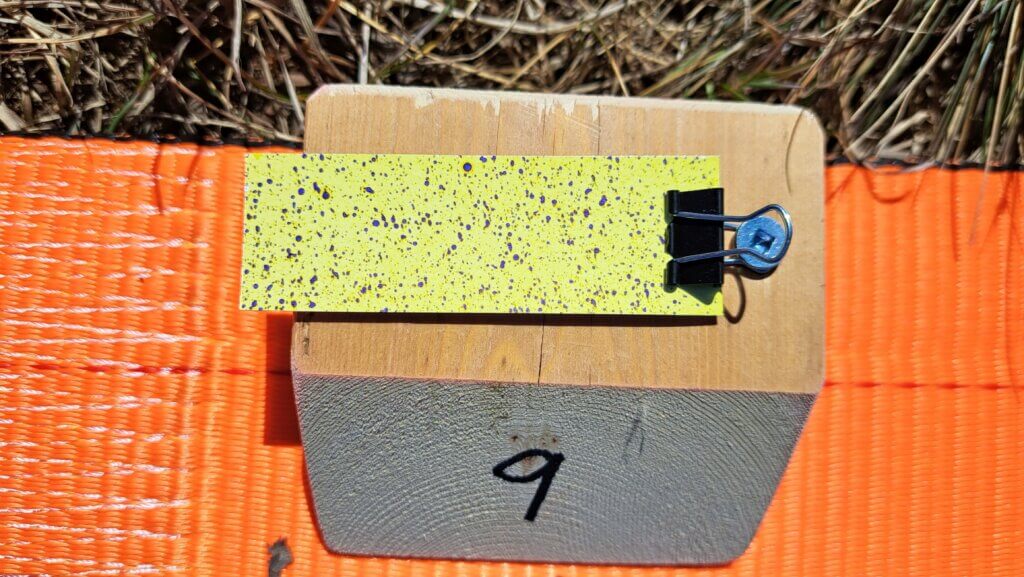
They flew this first prototype over water sensitive papers. Dropping from a 3 m (10 ft) altitude to 2 m (6.6 ft) improved coverage uniformity and resulted in a 10.3 m (34 ft) effective swath width. They could see the downwash was interfering with deposition, and while increasing to a larger droplet size helped, it didn’t help enough. Then they made some design changes, extending the boom 30.5 cm (12 in) beyond the rotors, and they saw they had something. They reached out to Agri-Spray Consulting (Nebraska) and arranged to run a series of Operation S.A.F.E. fly-ins.
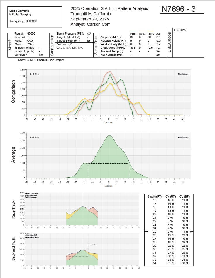
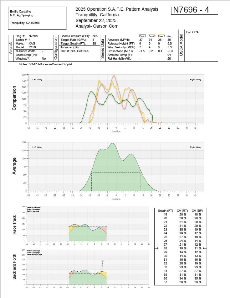
There were more than 25 flights that day, so we’ll focus on three specific load-outs. The critical parameters are listed in the following table in the order that they flew them. The first load-out (N7696-01) was deemed the best, and was the only one with the boom extended out front, beyond the rotor tips. This information is italicized. The other two are included here for interest. N7696-03 attempted to shift the boom back under the drone for cosmetic reasons, but also for ease of transportation. N7696-04 was the same configuration as the last, but with coarser droplets in an attempt to battle the downwash. The first fly-in report (N7696-01) is shown below, but all three reports can be downloaded by clicking the links above.
| Load-Out | Boom Position | Volume | Speed | Droplet Size (µm) | Altitude | Wind Velocity | Effective Swath Width | C.V. (Race Track / Back & Forth) |
| N7696-01 | Beyond Rotors | 50 L/ha (5 gpa) | 16 m/s (36 mph) | 230 | 2.75 m (9 ft) | 10.7 kmh (6.7 mph) | 10 m (33 ft) | 10%/10% |
| N7696-03 | Beneath Rotors | 50 L/ha (5 gpa) | 16.5 m/s (37 mph) | 230 | 2.75 m (9 ft) | 12.5 kmh (7.7 mph) | 7.6 m (25 ft) | 9%/11% |
| N7696-04 | Beneath Rotors | 50 L/ha (5 gpa) | 14.3 m/s (32 mph) | 400 | 2.75 m (9 ft) | 8.5 kmh (5.3 mph) | 8.5 m (28 ft) | 18%/11% |
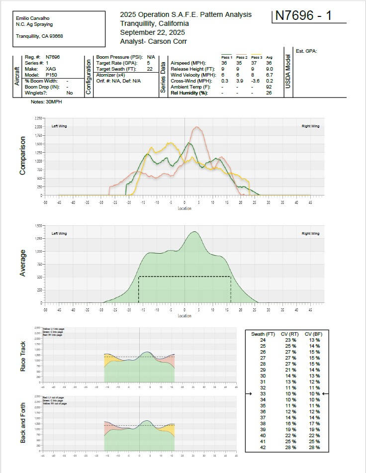
Observers said it looked like the swath was rolled with a paintbrush and that there were no observable vortices – just a sheet of spray. The following videos show some of the passes from that day. Actually, you can see vortices, but only in the passes where the boom is positioned beneath the rotors and not when it’s extended out front.
A 10% CV is spectacular, and the profile of each pass (even before averaging) was far flatter than any drone deposition I’ve seen previously. This design has not yet been used for custom application because there are still questions about how flight speed and pump flow will affect performance. But, the Carvalhos are already discussing the next design, constructed with carbon fibre tubes.
Impacts and Musings
Perhaps our description of how the air is moving over the drone is correct, or perhaps it isn’t quite right. Dr. Fernando Kassis Carvalho (no relation to Nino and Emilio) (AgroEfetiva, Sao Paulo, Brazil) recently shared that he also observed swath width no longer changed at speeds exceeding 13 or 14 m/s (personal communication). So, whatever the aerodynamic cause, the result seems clear.
Does this mean we’ll see a new generation of quadcopters with front mounted booms? It’s certainly possible, and kind of poetic as some early drone designs featured a centrally-mounted boom that extended beyond the rotor tips. Emilio wondered aloud about possible wear on the front motors, and likely there will be other issues as they experiment, but it’s early days and they’re enthusiastic about pursuing the design.
Nozzle Design
Should we also consider a return to hydraulic nozzles? The rotary atomizers on a drone currently leave a lot to be desired. Dr. Ulisses Antuniassi (Prof., Sao Paulo State University) studied the spray quality produced by rotary atomizers. He ran atomizers from a DJI T40 and from a XAG P60 in a wind tunnel spraying WG and SL formulations with either MSO or NIS adjuvants and found no logical trends in VMD, relative span or DV 0.1
Further, work by Dr. Steven Fredericks (Land O’Lakes) showed that the rotary atomizer from a DJI T40 created droplets roughly one ASABE category smaller than the software indicated. Conversely, common knowledge is that the XAG P100 version produces a coarser spray quality than anticipated, and slow motion video produced by Mark Ledebuhr (Application Insight LLC) and Dr. Michael Reinke (Michigan State University) clearly showed the flooding issue reported by Dr. Andrew Hewitt (University of Queensland), where excessive flow to the disc interferes with its ability produce a uniform droplet size.
I photographed no less than nine different rotary atomizer designs while at the End-User meeting. So, perhaps we should embrace a standardized design, or perhaps hydraulic nozzles should make a comeback. If the later, it would be a great opportunity to include PWM to increase their flow range.
Acceleration and Flight Pattern
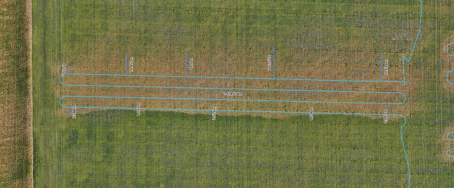
And what of kinematics? A drone’s “acceleration time” is calculated by dividing the change in velocity by the acceleration rate. We’ve seen that a DJI T100 must travel up to 100 m before it reaches target velocity. Admittedly, it was full and attempting to fly at high speed. Kevin Falk (Corteva Agriscience) noted a 25 m acceleration distance and a 15 m deceleration distance for a T50 flying mostly-full at 6 m/s. That’s a not-insignificant distance to achieve target flight speed.
What happens to the spray from a quadcopter drone with a front mounted boom as it transitions through the stages of flight? We don’t know for sure, but we can infer an inconsistent swath. Perhaps the prolonged acceleration time is sufficient reason for drones to start flying racetrack flight patterns like planes and helicopters, where they reach sufficient speed before passing over and spraying the target area. Current software does not allow that practice.
All this to say that as drone design continues to evolve, we must continue to challenge and test assumptions surrounding best practices. It has been fascinating to see how spray drones are finding their place in Western crop protection systems.
Acknowledgements
Thanks to Mark Ledebuhr (Application Insight LLC), Dr. Michael Reinke (Michigan State University), Kevin Falk (Corteva Agriscience), Dr. Tom Wolf (Application Research & Training), Adrian Rivard (Drone Spray Canada), and Adam Pfeffer (Bayer Crop Science) for insightful discussions.
Special thanks to Nino and Emilio Carvalho (NC Ag Spraying) for sharing their experience and practical approach to improving drone spray deposition.
Additional Resource
In early February, 2026, I gave a short interview with RealAgriculture. We discussed the state of spray application by drone in Canada as well as some of the possible impacts of higher speeds.


