Category: Nozzles & Droplets

Articles about nozzles and droplet size for specialty sprayers.

Pesticide Redistribution: An Important Aspect of Synthetic Pesticides
If you’re a sprayer operator with some experience behind you, you may have applied mercury arsenate, nicotine, Paris green, or perhaps even DDT. All of these historical pesticides were effective, but they were also toxic to both the applicators and the environment. Fortunately, today’s agrochemical manufacturers produce pesticides that are effective while being far less hazardous.
One important aspect of modern synthetic pesticides that enhances their efficacy is their ability to redistribute. Pesticide redistribution is the movement of a pesticide from its initial point of deposition to a different spot on or in the plant. Pesticides that can redistribute can improve pest control compared to those that must contact the target pest but cannot innately redistribute. This is especially true when spraying hard-to-wet plant tissues, such as flower clusters or fruit. Even when the immediate coverage of these tissues is insufficient, the subsequent relocation beyond the initial spray deposit can result in a more effective protective barrier. When plants are rapidly growing, many of these products can translocate through the plant tissues to protect newly emerged tissue that did not receive a direct deposit.
Some of the most difficult and persistent pests are more effectively controlled by redistributing pesticides. Materials that move within the plant after application provide improved control of piercing-sucking insects such as aphids and psyllids, as well as pests that feed in difficult-to-spray areas such as under leaves. These products can absorb into plant tissue, increasing their resistance to wash-off by rain or irrigation.
Five Types of Pesticide Redistribution
There are five significant types of pesticide redistribution: translaminar, vapor, xylem, phloem and redistribution via precipitation
Translaminar Redistribution
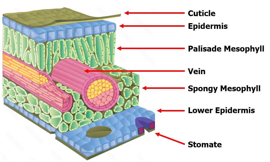
Translaminar redistribution (Figure 1) in its most literal sense is a compound moving from the side of the leaf that received spray, to the unsprayed opposite side. This results in protection on both sides. However, translaminar redistribution also involves limited radial movement providing a “halo” of protection around the initial deposition. The extent of this area of influence is product-dependent.
Figure 1. Schematic of translaminar redistribution, with small round dots indicating deposition of pesticide, arrows indicating the direction of redistribution, and the shading indicating the area of the plant protected by the pesticide.
Vapor Redistribution
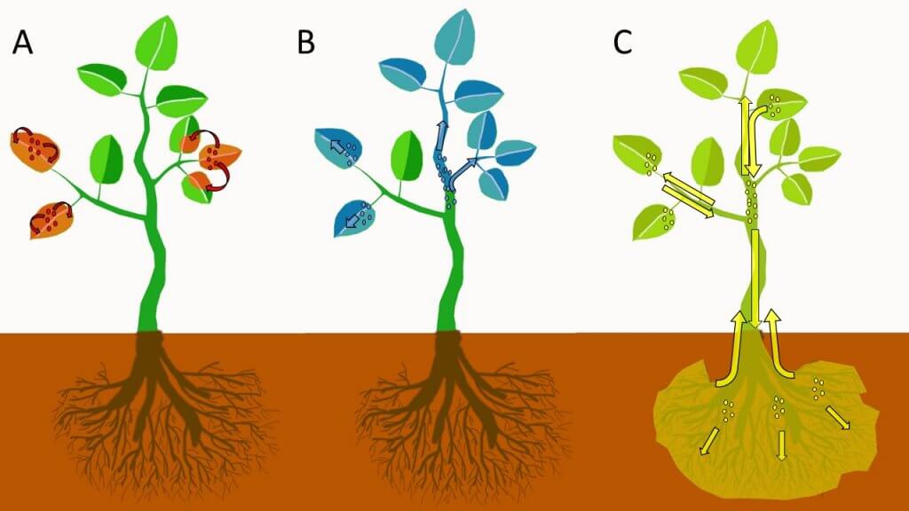
Vapor redistribution (Figure 2A) occurs when surface depositions volatilize and move laterally along a plant surface, re-adsorbing to the plant surface in new locations as they move. Again, the extent of vapor activity is product specific, but also condition specific requiring an optimal combination of temperature, relative humidity, wind, and solar radiation to facilitate volatilization. When pesticides are referred to as “locally systemic,” it often implies that they exhibit translaminar and/or vapor redistribution properties.
Figure 2. Pesticide redistribution type schematics (A) vapor, (B) xylem, (C) phloem. The small colored groups of dots indicate deposition of pesticide, while arrows indicate the direction of redistribution, with shading representing the area of the plant protected by the pesticide.
Xylem and Phloem Redistribution
Xylem redistribution (Figure 2B), also called xylem systemic, refers to the absorption of a pesticide and subsequent systemic movement of the pesticide through the xylem vessels of a plant. Xylem vessels move water and minerals in an upward and outward direction in plants. There is very little movement of water and nutrients downwards or backwards along branches or leaves in xylem vessels. Xylem redistribution can help protect growing tissues from damage by pests or diseases when the pesticide redistributes from the point of application to the newly developing tissues. Most systemic fungicides and insecticides redistribute via the xylem.
Phloem redistribution (Figure 2C), also called phloem systemic, is the bi-directional movement of pesticides in the phloem vessels of a plant. Phloem vessels transport sugars and other nutrients both to the roots of plants and upwards and outwards to shoots and fruits/seeds. Phloem systemic pesticides are sometimes called “true systemic,” because they can translocate throughout the entire plant.
Some pesticides that redistribute via the xylem or phloem can be applied to the soil substrate to be absorbed by the roots and redistributed throughout the plant. The process of plant nutrients or pesticides being transported from one place to another within the plant is called translocation.
Soil-Applied Systemics
Several factors affect a pesticide’s ability to redistribute. These factors affect the speed of uptake, the duration and extent of translocation, and the amount of accumulation in plant tissue relative to the initial dose. For pesticides labeled for soil application, their uptake by plant roots and redistribution via xylem or phloem can lead to long residual efficacy of the product; Up to eight weeks or more depending on the product, plant, and soil. This is in contrast to foliar-applied products, where good residual efficacy could be expected to last two to three weeks depending on the product. However, foliar-applied products tend to provide a more rapid kill of target pests and a more rapid absorption and translocation of active ingredients.
For soil-applied systemic pesticides, the composition of the soil substrate can affect the uptake of the pesticide by the plant. Growing media high in organic matter (>30% bark or peat moss) can bind pesticides, making it difficult for plants to absorb them through roots and subsequently translocate via the plants vascular system. Soil applications of systemic materials should take place one to six weeks prior to the onset of the insect pest or pathogen. This allows sufficient time for the pesticide to translocate to, and accumulate in, target tissues. The more water-soluble pesticides (e.g. Thiamethoxam) are taken up more rapidly than the less water-soluble pesticides (e.g. Imidacloprid).
Redistribution via Precipitation
In contrast to systemic pesticides, contact pesticides cannot redistribute on their own. However, rain or irrigation can spread the deposit to some degree, increasing coverage area. This effect should not be relied upon, as it depends on the product formulation, the intensity of the precipitation, and the interval following application. In the case of prolonged precipitation, the residual activity of contact products can be greatly reduced as they are diluted and washed off plant tissues.
Plant Morphology
The status of the plant to which they are being applied is a significant consideration when applying redistributing pesticides. Both soil-applied and foliar-applied pesticides are more rapidly absorbed and redistributed when applied to young plants or juvenile plant tissue. In general, when plants are actively growing, have a strong root system, or are actively transpiring, they tend to absorb and translocate pesticides more rapidly than when plants are growing slowly. In addition, plants with difficult to wet leaves or surfaces due to thick cuticles or waxy layers tend to not absorb pesticides as readily. Penetration into plants with difficult to wet surfaces can be improved by adding adjuvants such as surfactants to tank mixes.
Multiple Modes of Redistribution
The extent to which each product can redistribute can be thought of as a continuum. Generally, when a product exhibits some form of redistribution, it can also redistribute via a different method. A good example of this is xylem and translaminar redistribution. When a product can redistribute via the xylem it generally can move through the leaf via the translaminar pathway as well. Some products can redistribute via the xylem, translaminar, and vapor pathways all at the same time. Others, while technically able to redistribute via more than one mechanism, are only biologically effective via one mechanism.
Consult the Pesticide Label and Other Reputable Sources
The best way to determine how a pesticide product redistributes is to consult the manufacturer’s label, as well as technical information from reputable sources such as government or academia. If a manufacturer provides a technical information bulletin it is generally available on their website on the pesticide product page along with the label. However, because there are no standardized metrics to rate pesticide redistribution, there can be significant disparity between products. Some products that are advertised as being xylem systemic for example, are actually less systemic than products that are not even advertised as being systemic. Additional information on the efficacy and redistributing characteristics of specific products can be obtained from extension agents or crop consultants.
Conclusion
In summary, when selecting a pesticide remember to consider the four different pathways of redistribution (xylem, phloem, translaminar, and vapor) and how these methods may improve the efficacy of your application, allowing you to get more out of every drop.
January 25, 2022

Spraying Ginseng with Arag Microjets

In June 2013 we ran a ginseng spraying workshop and we learned as much as the growers did. Ginseng is notoriously difficult to spray:

It is highly susceptible to pathogens given the high humidity and still conditions generally found under the shade structure.
It forms a solid ceiling of leaves that resist spray penetrating to the stem and crown below and makes under-leaf coverage very difficult to achieve.

Many growers have (wisely) walked away from the old Casotti sprayers, which have been shown to give erratic coverage at best. They have adopted the Arag Microjet system with it’s characteristic orange shields. The >$80.00 CAD price tag for each nozzle is due to the brass mixing valve and swivel joint, as well as import costs from Italy. Contrary to popular belief, it does not use air-assist, or air-induction – it is strictly hydraulic. It does tend to create a ‘wake’ of air movement at high pressure. This phenomenon is called air entrainment and it is caused by large droplets travelling at high speed.

This nozzle is essentially the business-end of a spray gun. The way it is used in ginseng it works more-or-less like a hollow cone disc-core assembly. This begs the question “Why not use the cheaper and more readily available ceramic disc-core?” We set out to compare the two options using water sensitive paper set within the canopy. These yellow, paper targets turn blue when sprayed, clearly showing spray coverage.

Location of water-sensitive papers in the ginseng canopy. — Location of water sensitive papers in the ginseng canopy.

Determining rates

The first step was to determine the output rate for each nozzle. Generally, nozzle manufacturers provide rate tables showing how much volume a nozzle emits by time (e.g. US gallons per minute) at a given pressure. Finding these tables for the 1.5 millimetre Arag Microjet proved difficult. When we finally found one, it was discovered the rates were established for 200 to 850 pounds per square inch. This is excessively high pressure for a typical boom sprayer, so tables had to be developed for lower pressures.

Classic Arag microjets have a mixing valve that opens the spray up into a hollow cone, or collapses it into a tight stream. This also changes the rate. It can never be shut off completely, and it's hard to adjust consistently. — Classic Arag microjets have a mixing valve that opens the spray up into a hollow cone (valve handle left or right), or collapses it into a tight stream (valve handle middle). The valve position also changes the rate. It can never be shut off completely, and it’s hard to adjust consistently.

Determining nozzle rate using the Innoquest Spot-On SC-4.

Further, given the odd design of the mixing valve, it was determined that moving the handle ~10 degrees left of centre, or ~10 degrees right of centre, gave a difference of as much as 60%. The table below shows the outputs for a 1.5 millimetre nozzle with the handle in both positions and the two graphs show the results… well… graphically. Outputs were determined using the Innoquest Spot-On SC-4, but the frothing effect created by the nozzles may have created minor errors. Each rate is the average of a minimum of three samples.

Valve Setting	Pressure (psi)	Avg Output (gpm)	Pressure (bar)	Avg Output (L/min)
10 degrees left	40	1.02	2.76	3.86
10 degrees left	50	1.1	3.45	4.16
10 degrees left	60	1.25	4.14	4.73
10 degrees left	70	1.25	4.83	4.73
10 degrees left	80	1.38	5.52	5.22
10 degrees left	90	1.4	6.21	5.3
10 degrees left	100	1.45	6.89	5.49
10 degrees left	110	1.6	7.58	6.06
10 degrees left	120	1.75	8.27	6.62
10 degrees left	150	1.87	10.34	7.08
10 degrees left	200	2.2	13.79	8.33
10 degrees right	40	0.65	2.76	2.46
10 degrees right	50	0.7	3.45	2.65
10 degrees right	60	0.8	4.14	3.03
10 degrees right	70	0.85	4.83	3.22
10 degrees right	80	0.9	5.52	3.41
10 degrees right	90	0.9	6.21	3.41
10 degrees right	100	1	6.89	3.79
10 degrees right	110	1.07	7.58	4.05
10 degrees right	120	1.1	8.27	4.16
10 degrees right	150	1.25	10.34	4.73
10 degrees right	200	1.37	13.79	5.19

Average 1.5 mm ARAG Microjet output at a range of pressures and two valve settings in US Imperial units.

Average 1.5 mm ARAG Microjet output at a range of pressures and two valve settings in Metric units.

Comparing nozzles

Using the grower’s typical ground speed of 5 km/h (~3 mph) and operating pressure of 6.9 bar (100 psi), we found four TeeJet disc-core combinations that emitted a hollow cone pattern and approximately the same output as the Arag Microjets. The five nozzles sets tested were:

ARAG Microjet® 1.5 mm = ~0.95 US g/min avg at 100 psi
TeeJet® D8-DC25= 0.97 US g/min at 100 psi= ~97° cone
TeeJet®D7-DC45= 0.97 US g/min at 100 psi= ~81° cone
TeeJet®D4-DC46= 0.88 US g/min at 100 psi= ~33° cone
TeeJet®D6-DC45= 0.93 US g/min at 100 psi= ~81° cone

We did not use nozzle drop hoses (aka drop arms or hose drops) because it has already been firmly established that they are absolutely required to achieve under leaf coverage See OMAFRA factsheet 10-079 and this article.

Observations

While there were some complications with setting up the papers for the demo, we observed the following:

The output of each Microjet nozzle can be as much as 50% more or less than expected without being visually detectable and output for each nozzle must be confirmed before spraying. Therefore, outputs should be confirmed before every application.
Microjets at 100 psi emitting ~890 L/ha (~95 US gallons per acre) gave satisfactory coverage on all upward facing targets, but unsatisfactory under-leaf coverage. This has been demonstrated many times before.
The TeeJet D7-DC45 combination emitting a similar rate gave satisfactory coverage on all upward facing targets, but unsatisfactory under-leaf coverage. They may be a viable alternative to the Microjets.
Nozzle drops are advised to achieve under-leaf coverage.

The demo also raised some questions:

Did the TeeJet disc-core push the canopy apart as much as the Microjet? The audience noticed there was some leaf-shadowing where the cards did not get complete coverage using disc-core. This might have been coincidence, or it may not have. This question will be addressed in a research trial next season, but for now, the D7-DC45 appeared to give similar coverage to the Microjet.
Can nozzle drops be avoided if pressure is raised to 27.5 bar (400 psi)? Thanks to one grower trying this experiment in his garden after the demo, we saw some under-leaf coverage is possible at such high pressures, but this occurred at the cost of a lot of noise, diesel fuel and considerable wear on the ceramic Microjet discs. The grower tested these tips and discovered they needed replacement after only two years of use. Nozzle drops are cheaper, easier and result in considerably more spray in the under leaf positions.
We saw what minimal and excessive foliar coverage looked like, and determined how much variability there was from one nozzle to another. A significant question was “How much spray can be saved when using a more accurate application?” and the answer is yet to be determined, but could be well in excess of 10% of the typical spray volume. Given that this crop can be sprayed more than 100 times over it’s 3 or four years before harvest, this represents significant savings in pesticides and refill time.

Additional – Newer ARAG Microjet Design

Since this work was performed, growers have been exploring a newer option from ARAG.

They are an improvement over the older version insofar as they are more easily calibrated and held at a given rate thanks to a lock nut. They still employ a 1.5 mm diameter ceramic disc, but this can be changed for a 1.0 or 1.2 quite easily. They are still somewhat finicky when trying to set a consistent spray quality and rate from nozzle to nozzle, but are better than the mixing-valve option.

Learn more in this article.

Custom-made ginseng sprayer. A standard design. — Custom-made ginseng sprayer. A standard design with newer, cheaper and easier-to-use ARAG microjets.

Special thanks to Syngenta Canada for providing lunch, to C&R Atkinson Farms Ltd. for hosting, to TeeJet for supplying the disc-cores and water-sensitive papers, and to Dr. Sean Westerveld, Dr. Melanie Filotas and OMAFRA summer student Megan Leedham for contributing to the workshop.

September 7, 2021

Assessing Water Sensitive Paper – Part 3
This is the final part of our three-part article discussing methods for digitizing and processing water sensitive paper. You can read part one here and part two here.
Morphological operations
We can now move on to the larger shapes, or “morphology” of the objects in our binary image. Our goal is to quantify deposits by interpreting these shapes. Once again, these operations are powerful processing tools, but we must acknowledge three overriding limitations:
1. Inconsistent stains
Sometimes deposits do not create a consistent blue colour – they can get lighter or take on a greenish-yellow hue towards the perimeter of the stain. During thresholding, the outer edge can be accidently eroded, leaving behind an object with a jagged edge. This may lead us to underestimate the percent area actually covered. In the case of tiny stains, it might eliminate them entirely and lead us to underestimate deposit density.
2. Overlaps
It can be difficult to determine if an object represents a stain from a single droplet or is the result of multiple, overlapping deposits. This becomes significant when the surface of the WSP exceeds ~20% total coverage. The resulting objects may or may not have hollow centres where droplets do not overlap entirely. Misidentifying overlaps leads us to falsely conclude that an object is the result of a single, coarser droplet rather than multiple finer droplets.
3. Ellipses
Non-circular stains are formed when droplets scuff along the surface. Two droplets with the same volume encountering a paper at different angles can create stains with significantly different areas. We may wrongly conclude that the droplets that created them were coarser than they truly were. One approach is to use Feret’s Diameter (aka Caliper Diameter) by measuring the widest spans on the X and Y axes and taking the average. Another approach is to interpret the ellipse as a series of circular stains. Or we can decide to only acknowledge these objects when calculating percent area covered, but omit them when calculating deposit density or predicting original droplet size. Each strategy is a compromise, so it is important to be consistent and transparent when reporting results.
Three common problems when analysing water sensitive paper.
We’ll explore two morphological operations that can help us separate fact from fiction: Granulometry and Dilation-and-Erosion. We’re introducing these operations as part of the processing and detection step, but they may also overlap with the measurement step in our three-step process.
Granulometry
We can estimate the range of object sizes and get a sense of how they are distributed on the paper by filtering or “sieving” the image. Imagine pouring a mixture of sand and rocks through a series of ever-finer sieves. Doing so allows you to separate particles based on size exclusion. A granulometry function compares each object to a series of standardized objects with decreasing diameters. This isolates objects of a similar size and bins them in that size range. This is a powerful operation, but accuracy is lost when stains overlap to form larger objects. In this case, we move on to Dilation and Erosion.
Dilation and Erosion
Think of dilation as adding pixels to the boundary of an object. This makes tiny objects bigger, fills in any interior holes and can cause objects to merge. The number of pixel-wide dilations required to make objects contact one another can be used as a measure of deposit density.
Erosion removes pixels from the outer (and sometimes inner) boundaries of an object. This eliminates tiny artifacts that may not actually represent stains. It can also split non-circular objects into multiple parts before shrinking them into multiple nuclei (aka centroids). These last-remaining points are not necessarily the centre of a stain, but the pixels furthest away from the original boundary.
When a non-circular shape has more than one nucleus, they likely represent individual droplets that combined to form the larger stain. We can then use these nuclei to measure deposit density, such as in a Voronoi partition which triangulates each nucleus in relation to the two closest neighbours.
Many image processers use both these operations sequentially. When an image is eroded and then dilated (a process called “Opening”), smaller objects are removed, leaving the area and shape of remaining objects relatively intact. Dilating and then eroding (a process called “Closing”) fills in small holes and merges smaller objects, once again leaving the area and shape of remaining objects relatively intact. We can use both of these functions to help smooth an image prior to measurement.
(Top) Opening operations erode and then dilate the image. Moving left to right, the smaller objects tend to disappear. (Bottom) Closing operations dilate and then erode the image. Moving left to right, smaller objects either disappear or merge and holes are filled in
Distance Transformations
Distance transformations are advanced operations specifically used to separate objects that are densely packed. While not typically used when analyzing WSP, distance transformations are another means of identifying object nuclei. They are another means for teasing apart objects that are likely the result of overlapping deposits and then mapping their relative sizes and positions.
Measurement
The calculation of the area covered by deposits is straightforward. The pixels belonging to objects (the deposits) and those belonging to background are summed and then the fraction is converted to percent area covered. Research has shown that the image resolution does not significantly impact percent coverage assessments and has suggested that all image analysis software tends to produce similar results (+/- 3.5% observed when the same threshold was applied to multiple papers). This is acceptable because it’s within the variability inherent to spraying.
We ran a similar experiment wherein we analyzed the same piece of WSP using four methods. Here are a few facts about the software we used:
- DropScope produces images between 2,100 and 2,300 DPI. Currently, it ignores ellipses and doesn’t count anything spanning less than ~35 µm (3 pixels).
- We set ImageJ to ignore any object spanning less than 3 pixels, which at 2,400 DPI was 30 µm in diameter.
- We are unaware of Snapcard’s processing methods except that the software was benchmarked using ImageJ. Developers note it will underestimate the percent area covered if the image is out of focus. (Note: As of 2026, this app may no longer be supported by the GRDC).
The images shown in the figure below were cropped from screenshots produced by each method. The actual ROI analyzed was ~3 cm² for SnapCard, 3.68 cm² for DropScope and 2.0 cm² for both Epson/ImageJ methods. Our results indicate an +/- 4% difference in percent area coverage. This variability reflects the results of a 2016 journal article that compared SnapCard with ImageJ and other leading analytical software. That study claimed no statistically significant difference in percent coverage detected (standard deviations were about 20%). However, the ImageJ results tended to trend several percent higher than SnapCard. We saw this as well. And so, while resolution may not have a significant impact on percent area covered, there does appear to be some correlation.
Percent area covered as reported by three image analysis systems. Only a minor difference was observed when resolution was doubled using the Epson/ImageJ method.
Resolution definitely affects deposit counts. Particularly in applications that employ finer droplets. Consider the difference between detecting or missing 1,000 30 µm diameter objects. It may only amount to a fraction of a percentage of the surface covered, but +/- 1,000 objects on a 2 cm² area is significant in terms of deposit density.
Output
Once a WSP image (or set of images) has been scanned, pre-processed, processed and measured, we will receive some manner of output. Some software packages create an attractive report with images, graphs and key values. These reports include percent coverage and many provide droplet density. Deposits may be binned by size, or spread factors are used to calculate the original droplet diameters and even estimate the volume applied by area. Other software packages provide raw data that can be imported into a statistical program or spreadsheet program like Excel for further analysis. Some software packages provide both.
How far can we take this?
Blow-by-blow data analysis is beyond the scope of this document, but how much weight should we give to coverage data obtained using WSP? The answer depends on the metric in question, but in all cases we must first acknowledge the three overriding caveats. Take it as said that they apply to everything that follows:
1. Different brands (and even different production runs) of WSP can produce significantly different coverage metrics. When conducting experiments, use a single brand of WSP. Better still, use papers from the same production batch whenever possible.
2. The same of piece of sprayed WSP can produce significantly different results depending on the software and protocol used to analyze it. When conducting experiments, use the same software and assessment protocol and be transparent about the process when communicating results.
3. WSP coverage may not reflect the coverage achieved on an actual plant tissue surface. It is suitable as a relative index (I.e. papers can be compared to papers, but not to tissues) but the spread factor changes with surface wettability and the surface tension of the liquid sprayed. Note the differences in percent area covered in the following experiment with an organosilicone super-spreader:
Difference in deposit spread on water sensitive paper versus a leaf surface using an organosilicone super-spreader and UV dye. The same volume was applied in each case and while the area increased two-fold on WSP it increased ~10-fold on an actual leaf. Image reproduced from work by Robyn Gaskin, Plant Protection Products, New Zealand.
Recall that we started this document by listing the four pieces of information commonly sought using WSP. They were listed in order of reliability, and now we can explain why.
- The percent surface area covered: We have established that this is the most reliable piece of data. Droplets do not spread on WSP the way they do on plant surfaces, so it will underestimate actual coverage. The results vary by analytical method, but it’s likely not dependent on resolution and still falls within the variability inherent to spraying. This metric gives us valuable and actionable information. We can say whether or not we hit a target, and evaluate whether a sprayer change resulted in more or less deposit.
- The density of deposits on the target area: We have established that that there are limits to the reliability of this metric. It is affected by the analytical method used and can be greatly underestimated when resolution is poor or when deposits overlap in high numbers. Also, it will never reliably reflect deposits under 30 µm. Nevertheless, under controlled conditions this information does have value and is of great interest in enquiries about drift and contact fungicides.
- The size of the droplets that left the stains: This metric is highly questionable except under controlled conditions. The many assumptions about surface tension, droplet speed, and droplet evaporation make it impossible to make definitive statements about spray quality. Finer droplets are greatly underestimated in this equation. Therefore, while there may be some value in using WSP as a relative index, this metric is a crude indication at best.
- The dose applied to the target surface: This metric has not been discussed up to this point, but is quickly and easily dismissed. Let’s assume that a droplet with a high concentration of an active ingredient will leave a stain that is the same area as another droplet with a lower concentration. This will lead some to suggest that as long as the original concentration is known, we can back-calculate the dose (which is the amount of active on a given area). However, one droplet has the same volume as eight droplets that are half it’s diameter. This cubic relationship means that if they all deposit, the larger droplet will cover roughly 1/2 the surface area as the eight smaller droplets. Therefore, the smaller droplets spread the same amount of active over a greater area. Spread factor muddies this a bit, but ultimately it means that dose cannot be estimated from area covered. Dose is better assessed using collectors that permit the residue to be removed, such as Petri dishes, Mylar sheets, pipe cleaners, alpha cellulose cards, or glass slides.
And so, the image analysis process described here is powerful and effective when used with water sensitive paper as long as the limitations are acknowledged. The same process can also be used with dyes and specialized collectors such as Kromekote to permit even greater resolution. But that’s another story.
References (Further reading)
Bankhead, P. 2014. Analyzing fluorescence microscopy images with ImageJ.
Cunha, J.P.A.R., Farnese, A.C., Olivet, J.J. 2013. Computer programs for analysis of droplets sprayed on water sensitive papers. Planta Daninha, Viçosa-MG. 31(3): 715-720.
Ferguson, J.C., Chechetto, R.G., O’Donnell, C.C., Fritz, B.K., Hoffmann, W.C., Coleman, C.E., Chauhan, B.S., Adkins, S.W. Kruger, G.R., Hewitt, A.J. 2016. Assessing a novel smartphone application – SnapCard, compared to five imaging systems to quantify droplet deposition on artificial collectors. Computers and Electronics in Agriculture. 128: 193-198.
Ledebuhr, M. 2016. Small Drop Sprays.
Marçal, A.R.S., Cunha, M. 2008. Image processing of artificial targets for automatic evaluation of spray targets. Trans. of the ASABE. 51(3): 811-821.
Moor, A., Langenakens, J., Vereecke, E., Jaeken, P., Lootens, P., Vandecasteele, P. 2000. Image analysis of water sensitive paper as a tool for the evaluation of spray distribution of orchard sprayers. Aspects of Applied Biology. 57.
Panneton, B. 2002. Image analysis of water‐sensitive cards for spray coverage experiments. Applied Eng. in Agric. 18(2): 179‐182.
Salyani, M., Zhu, H., Sweeb, R.D., Pai, N. 2013. Assessment of spray distribution with water-sensitive paper. Agric. Eng. Int.: CIGR Journal. 15(2): 101-111.
SnapCard website. University of Western Australia and the Department of Primary Industries and Regional Development, Western Australia. (Note: As of 2026, may no longer exist).
Syngenta. 2002. Water‐sensitive paper for monitoring spray distributions. CH‐4002. Basle, Switzerland: Syngenta Crop Protection.
Turner, C.R., Huntington, K.A. 1970. The use of a water sensitive dye for the detection and assessment of small spray droplets. J. Agric. Eng. Res. 15: 385-387.
July 27, 2021
Ten Tips for Spraying in the Wind
Choosing the right time to spray can be tricky. Our gut tells us that spraying when it’s windy is wrong. The experts tell us that spraying when it’s calm is wrong. So when can you actually spray?
I’ve always advised my clients to spray in some wind, because it has a few advantages. The main one is that wind helps disperse the spray upward and downward, diluting the spray cloud fairly rapidly. Another advantage is that winds tend to be reasonably steady in their direction and velocity (or at least that can be forecast), so downwind areas can be identified and potential impacts are known or predictable. It helps if it’s sunny, because that improves the dispersion of the cloud even more.
First, let’s define “windy”. The classic wind scale is the Beaufort Scale, intended for the sea, but also used on land. The upper limit for spraying is probably Force 3 or Force 4, with upper limits of 20 – 25 km/h or so. The Beaufort Scale calls these “Gentle or Moderate Breezes” (they had to save the alarming words for hurricanes), and the scale provides good visual clues such as what wind does to flags, leaves, or dust.
Spraying under breezy conditions can be done fairly safely if you follow specific steps. The idea is to understand what the risks are and to manage them.
The cornerstone is to use a low-drift spray and match it to a pesticide that will work well with larger droplets. But there are other important aspects to consider. Below are the top ten to think about:
- Choose a herbicide that can handle large droplets. Glyphosate products are well suited to coarse droplets. But glyphosate commonly has contact actives in the mix, members of Group 6, 14, and 15, and these are less likely to perform well with big droplets than those that contain Group 2 and 4 mixes. Actives with soil activity also have more tolerance for larger droplets.
- Use a low-drift nozzle and operate it so it produces a Coarse (C) to Very Coarse (VC) spray quality, as described by the manufacturer. Dicamba labels call for Extremely Coarse (XC) to Ultra-Coarse (UC) sprays, and Enlist requires at least Coarse. To achieve these you may need to purchase new nozzles. Low-pressure air-induced nozzles operated at about 50 – 60 psi will generally be very low-drift, but lower drift models are available. If you need a finer spray, produce it either by increasing the pressure or moving to a finer tip. Do this when the weather improves, for contact modes of action.
The name, symbol and range of droplet sizes used to describe the median droplet diameter produced by nozzles according to ASABE S572.3
- Keep your boom low. Lowering the boom ranks as the second-most effective way to reduce drift, after coarser sprays. But there’s a limit. For low-drift sprays, you need at least 100% overlap (more for PWM), which is for the edge of one nozzle pattern to spray into the centre of the adjacent pattern. In other words, the spray pattern should be twice as wide as your nozzle spacing at target height. For most nozzles, a boom height of close to 20 inches is enough to achieve this overlap. That’s pretty low by current standards from suspended booms on self-propelled sprayers, so being too low for a good pattern will only happen due to boom sway.
- Maintain reasonably slow travel speeds. These reduce the amount of fine droplets that hang behind the spray boom, reduce turbulence from sprayer wheels, and they also make low booms more practical. An added bonus is less dust generation.
- Know what’s downwind and what harms it. Survey the fields on all sides of the parcel you’re treating. When you have a choice, avoid spraying fields that have sensitive areas downwind such as water, shelterbelts, pastures, people, etc. If you can’t avoid being upwind of these areas, make sure you check and obey the buffer zone restrictions on the label. These will also give you an idea if the product can cause harm in water or on land, or both.
- Let the weather help you.
  1. Take the wind from the side if you can. Going straight into the wind creates a lot of extra drift.
  2. Spray when the sun shines if you have a choice. Early morning, late evening, or cloudy days increase the distance that drift moves. When it’s sunny, the drift cloud disperses quickly and causes less damage.
- Consider a dicamba tip for special situations, even if you don’t use dicamba. If you’re in a situation where quitting and waiting is a poor option, these tips allow you to finish the job with minimal drift risk and with only slight reductions in product performance due to poor coverage.
- Use a low-drift adjuvant. Specific products such as Interlock or Valid have been shown to reduce driftable fines (<150 microns) by between 40 – 60%, without adding significant volume in coarser droplets. The response will depend on the nozzle and the tank mix, but can be very noticeable.
- Study drift and how it forms and moves. It’s about more than wind speed and droplet size. Knowledge in this area can help you work out the best strategies.
- Invest in productivity. You may not need it every day, but on occasions when you have a small window to avoid bad weather, it pays dividends.
- If you feel that drift is unavoidable and someone might be impacted by it, talk to those people first. It’s one of the most important things you can do.
Keeping pesticide sprays on target continues to be one of our top responsibilities.
June 8, 2021
Spraying Asparagus in Fern
This research was performed in 2012 and since then there have been considerable advances in application technology for asparagus in fern that should be considered. Be sure to read the epilogue at the end of this article.
Introduction
Diseases such as purple spot can have major economic impacts for asparagus growers, and the best line of defence is spraying the appropriate control products. The good news is that asparagus growers know this. The bad news is that there are few things harder to spray than asparagus in fern.
Asparagus infected with purple spot.
Asparagus in fern can stand 1.5 m (5 ft) high by 1.0 m (3 ft) diameter and is typically planted on 1.2 m (4 ft) centres. Asparagus in fern has a very dense canopy full of needle-shaped leaves. This dense canopy slows air movement, making conditions still, humid and very difficult for a spray droplet to penetrate.
Spraying asparagus in fern.
Spray coverage is a combination of two factors: the area of the target contacted by spray droplets, and the distribution of spray droplets over that target. For most insecticide and fungicide applications, reasonable coverage is reflected by 10-15% surface area covered paired with an even distribution of approximately 85 medium sized droplets per square centimeter. This is not a rule, but a guideline.
In order to determine the best way to spray, we have to be able to compare the coverage achieved. To do this, we used water sensitive paper, which is yellow until contact with spray turns it blue. Three sets of three targets were placed in approximately the same location for each pass.
Water sensitive paper arranged on stands, ready to be placed in the fern.
Water sensitive paper orientation and location in asparagus canopy relative to sprayer direction.
We tested five popular nozzle types, at two ground speeds using three carrier volumes to answer three questions:
1. Does spray volume impact spray coverage?
2. Which nozzle style gives the best coverage?
3. Does travel speed impact spray coverage?
Does spray volume impact spray coverage?
Five different nozzle types were used to spray three volumes onto the targets at 16 kmh (10 mph). This was repeated three times and target coverage was determined both as droplet deposits per cm² (see Figure 1) and total % covered (see Figure 2).
Figure 1. Average deposits per cm^2 for five different nozzle types at 187 L/ha (20 US gpa), 234 L/ha (25 US gpa) and 280 L/ha (30 US gpa) at a ground speed of 16 kmh (10 mph).
Figure 2. Combined average percent coverage for five different nozzle types at 187 L/ha (20 US gpa), 234 L/ha (25 US gpa) and 280 L/ha (30 US gpa) at a ground speed of 16 kmh (10 mph).
Cards in each position consistently received a significantly higher average deposit per cm² and significantly higher average percent coverage at higher spray volumes. The relatively low coverage in the middle position was anticipated given the orientation of the targets to the sprayer.
Therefore, it would appear higher volumes result in better coverage, at least up to 280 L/ha (30 gpa). Generally, there is a threshold where exceeding a given carrier volume results in a diminishing return.
Which nozzle gives the best coverage?
Coverage from five different nozzles was compared: the Hollow cone, Flat fan, Dual flat fan, Guardian Air and Air-induced hollow cone. Given that 280 L/ha (30 gpa) resulted in the best coverage, the following figures illustrate droplet deposits per cm² (see Figure 3) and total % covered (see Figure 4) at 280 L/ha (30 gpa).
Figure 3. Average deposits per cm^2 for five different nozzle types at 280 L/ha (30 US gpa) and 16 kmh (10 mph).
Figure 4. Average percent coverage for five different nozzle types at 280 L/ha (30 US gpa) and 16 kmh (10 mph).
The graphs show that each nozzle followed a similar trend, with more droplets at the top of the canopy, less or par at the bottom of the canopy, and considerably less in the middle of the canopy (which is not surprising given the orientation of the target around the stem).
The trend in droplet density from highest to least coverage is:
1. Hollow Cone
2. XR flat Fan
3. Guardian Air
4. Dual Flat Fan
5. Air Induced Hollow Cone
The percent coverage data was less clear. The top two nozzles for each position were:
Top Target:
1. Guardian Air
2. All other nozzles approximately the same
Middle Target (around the stem):
1. XR flat Fan
2. Hollow Cone
Bottom Target:
1. XR flat Fan
2. Hollow Cone
It can be argued that the target at the top of the canopy is easiest to spray, and therefore does not have as much importance as the middle and bottom targets. As such, it would appear that the XR flat fan and Hollow cone nozzles give the best overall coverage. It is debatable whether the higher droplet count from the Hollow cone is more important than the higher percent coverage of the XR flat fan.
Does travel speed impact spray coverage?
Hollow cone nozzles and XR flat fan nozzles were used to spray targets at two travel speeds and three volumes. Target coverage was determined both as droplet deposits per cm² (see Figure 5) and total % covered (see Figure 6).
Figure 5. Average deposits per cm^2 for Hollow cone and XR flat fan nozzles at 280 L/ha (30 US gpa) and either 8 kmh (5 mph) or 16 kmh (10 mph).
Figure 6. Average percent coverage for Hollow cone and XR Flat fan nozzles at 280 L/ha (30 US gpa) and either 8 kmh (5 mph) or 16 kmh (10 mph).
The variability in deposit density and percent coverage from medium/fine droplets created by the hollow cone nozzles make it difficult to determine statistical significance, but the trend suggests that higher ground speeds improve coverage in the middle and bottom of the canopy. This is likely due to the wake of the sprayer and the vortices created by its passage stirring fine droplets into the canopy.
Overall recommendations
The data suggest that coverage was improved when the sprayer travels at 16 kmh (10 mph) rather than 8 kmh (5 mph). Coverage was also improved at higher spray volumes, where 280 L/ha (30 US g/ac) provided the best overall coverage for all nozzles. As for the best nozzle, this depends on the application; the hollow cone created higher droplet densities than the XR flat fan, but the XR Flat fan created higher percent coverage. Higher droplet densities may be preferred when controlling disease with contact products, but spray drift becomes a significant concern. Higher percent coverage might be preferred with locally systemic products where complete coverage is less of a concern and preventing spray drift is a priority.
Epilogue
This work was performed in 2012. Since then there have been significant advances in sprayer design for spraying asparagus in fern. Dr. Torsten Balz (Bayer Application Technology Manager) kindly provided an example of such a sprayer (see below) and a video link to watch it in action. Drop arms that bring the nozzles closer to the target at all canopy depths are an ideal solution as long as the row spacing allows clearance without snagging the drops. Further, there have been developments regarding the use of hollow cones in an overhead broadcast application. Over- and under-laps in the hollow cone swath lead to double-dosing and gaps respectively that are referred to as “Technical Strip Disease”. Combined with considerable drift potential, hollow cones are not recommended.
Air-assisted drop arms greatly improve coverage uniformity in asparagus in fern. Photo kindly provided by Dr. Torsten Balz.
Special thanks to Max Underhill Farm Supply (Vienna, Ontario) for use of their sprayer and their assistance both spraying and placing water sensitive papers in the field. Thanks to Mr. Ken Wall of Sandy Shore Farms Ltd. (Port Burwell, Ontario) for providing the site and hosting the associated workshop, and thanks to TeeJet Technologies for their donation of parts and supplies.
June 3, 2021