The aesthetic value of ornamental plants requires a near-zero tolerance for insect pests, which cause up to 10% of crop losses per season. Controlling them with insecticides is a difficult proposition:
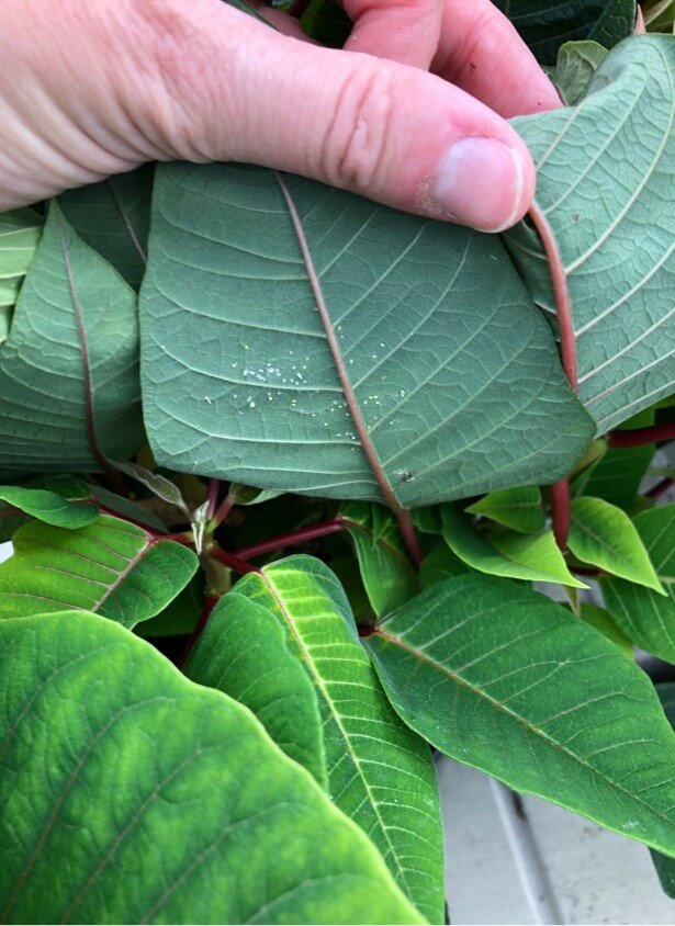
- Key pests such as thrips, aphids and whiteflies tend to feed on the underside of leaves – a notoriously difficult surface to target because of it’s orientation relative to the spray nozzle (see image below).
- Other pests, such as mealybugs, are found on stems. Stems are hard-to-wet plant surfaces because spray tends to run off. Further, as the plant canopy grows and densifies, these surfaces are buried deep inside, out of line-of-sight.
- The insecticides available for closed environment spraying must be compatible with biological controls and are therefore “softer” chemistries. Examples include soaps, oils and entomopathogenic fungi. These products require contact with the pest and are at best translaminar, so coverage becomes critical for performance.
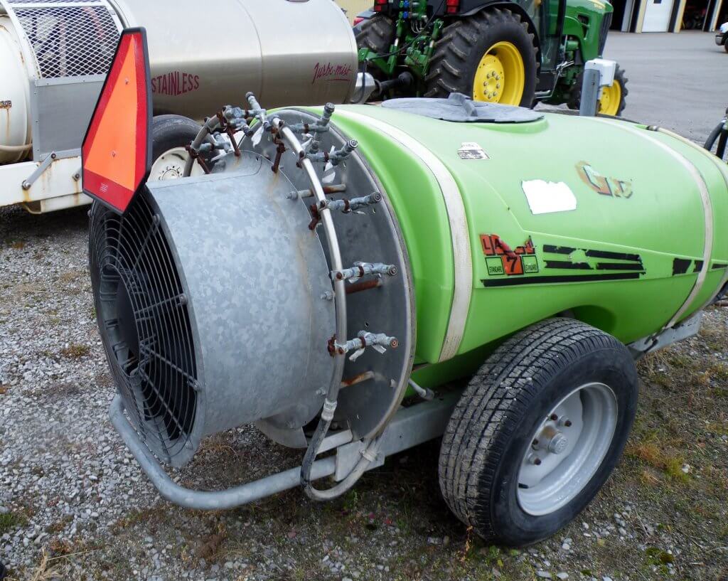
Spraying for Insects
The planting architectures and canopy morphologies are highly variable in ornamental greenhouses. Perhaps they are young plants with sparse canopies, densely packed in pots on raised tables. Perhaps they are mature, hanging plants with dense canopies. Perhaps they are something in between.
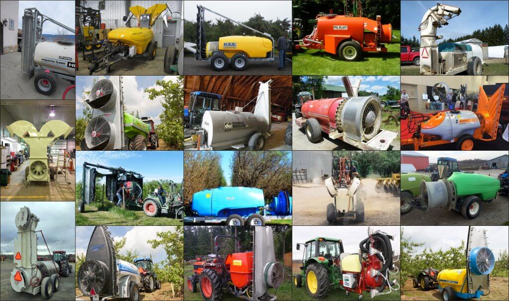
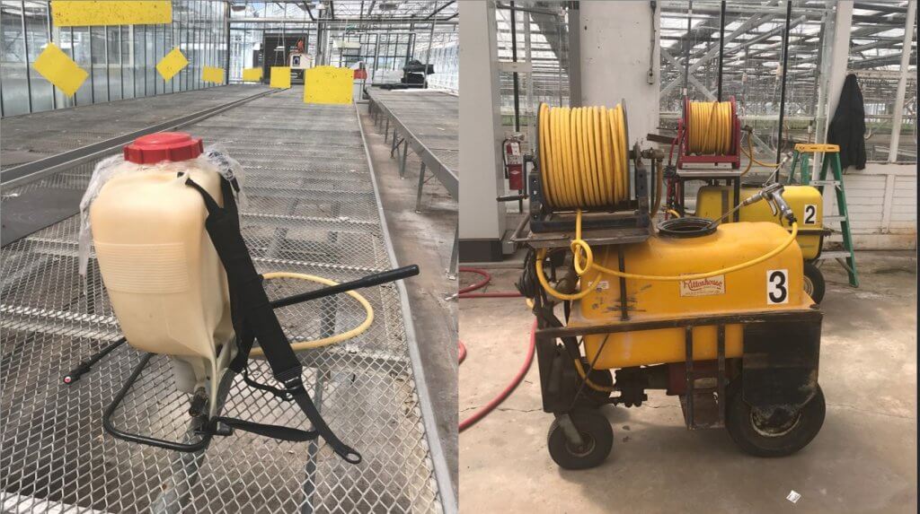
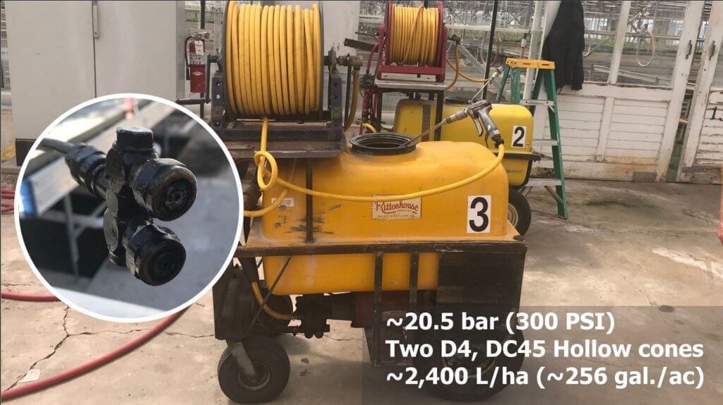
Ideally, each combination of canopy morphology, planting architecture, pest and chemistry would have a specific sprayer designed to optimize coverage and efficiency. This is economically unrealistic. Instead, many producers utilize technologies that rely on high water volumes and hydraulic pressures to “drench” targets indiscriminately. Others employ highly manual methods that allow the operator to aim the nozzle in relation to the canopy on a case-by-case basis, but still rely solely on water to distribute the insecticide.
These technologies have their place, but the reliance on hydraulic pressure and carrier volume has drawbacks:
- High water volumes lead to higher humidity in closed environments which may favour disease.
- The inevitable run-off creates waste water that may require treatment before leaving closed environments.
- High carrier volumes dilute an already “soft” chemistry and hydraulic pressure doesn’t always improve canopy penetration or coverage uniformity.
Air-assisted spraying can be a viable alternative (and an improvement) over these approaches. Stationary or mobile, many ultra-low volume sprayers already employ air to capitalize on the mechanical advantage offered by smaller and more numerous droplets. Finer droplets have very little mass, so they must be directed and carried by air currents to get them to the target. Sufficient air energy will also displace the air within the target canopy and physically expose otherwise hidden plant surfaces to the spray.
The upshot is that air can partially replace water as a carrier and it has the potential to improve coverage uniformity throughout the target canopy.
Testing Air-Assisted Spraying
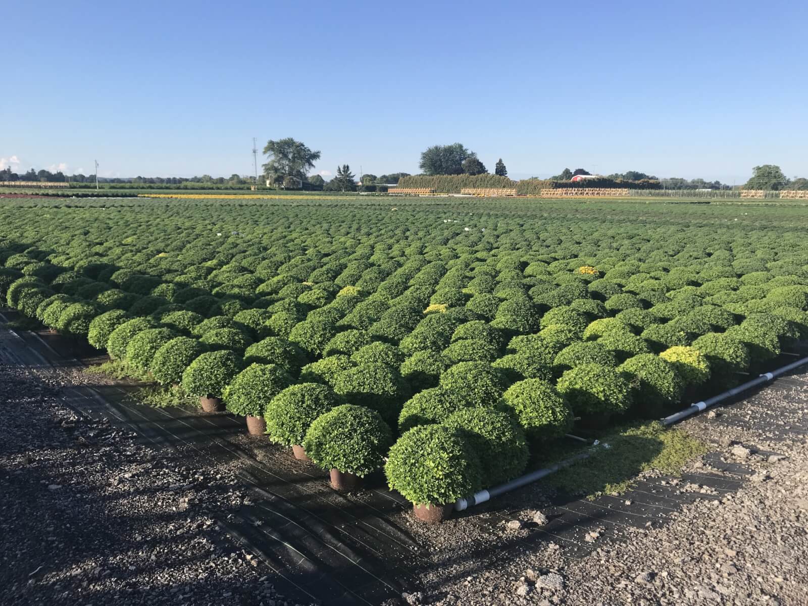
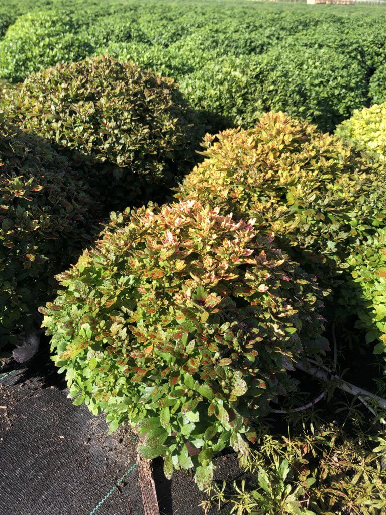
We chose to test this assertion in a chrysanthemum nursery. Our objective was to compare the coverage from the grower’s conventional hydraulic gun to that of a customized backpack mist blower.
Crop Canopy and Architecture
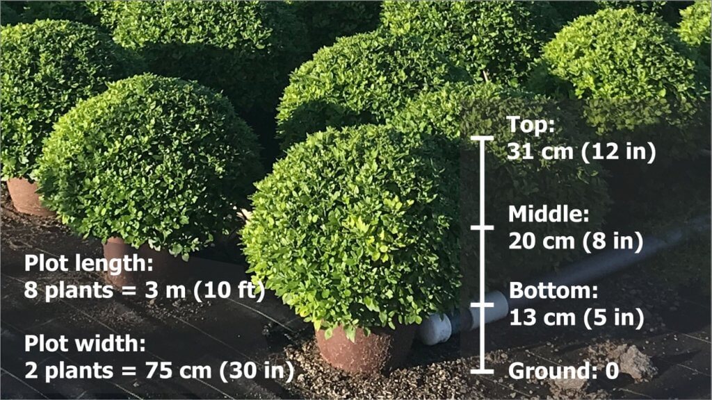
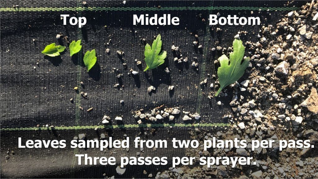
The crop canopy wasn’t fully mature but still represented a very dense target. In order to compare canopy penetration the canopy was divided into three depths: The Top exterior, the Middle (8″ from ground) and the Bottom (just above the pot soil). Each treatment area contained 8×2 plants and a buffer of three plants was maintained between treatments. We made three sprays (reps) for each condition.
Sprayers
Several attempts were made to redirect and redistribute air from a commercial backpack mist blower. The goal was to create an air outlet that would distribute the same air speed over a long and narrow swath. Air is highly compressible and early attempts using baffles, straightening vanes and variable outlet sizes were unsuccessful. A compromise was reached by reducing the swath to about plant-width (40 cm). This was confirmed by spraying water on dry pavement and measuring the width of the swath. While not ideal, the operator could span the full 75 cm plot width by shifting the outlet back-and-forth laterally while spraying. There are videos below that show examples of both applications.
Through trial and error, the outlet was held above the canopy at a height and angle that optimized air penetration. If the outlet was held too far away, there was insufficient air energy to penetrate the canopy. If held too close, too much spray-laden air would escape the canopy. These attempts were performed at a comfortable walking pace to account for dwell time (E.g., the longer the outlet remained stationary over a canopy, the deeper it penetrates).
The grower’s conventional sprayer was used according to their typical practices. Walking pace and flow rate were measured to establish application volume for both sprayers.
Coverage Indicator
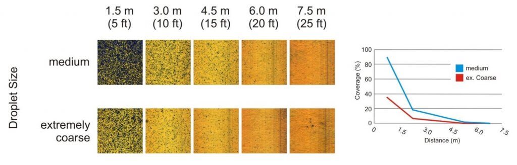
Coverage was quantified using dye recovery and fluorimetry. The process is described in detail in this article and this article. Basically, a known concentration of Rhodamine WT dye is applied to the plant. Sprayed leaves are collected from key locations in the canopy and placed in labelled containers with a known volume of water. Later, that water is analyzed in a fluorimeter and the data is normalized by leaf weight (or in this case, leaf surface area) to account for the volume used and the size of the leaf sampled.
In addition to dye recovery, we also used water sensitive paper as a qualitative indicator. Papers were placed at the Middle depth facing into and away from the direction of travel and sprayed with both methods. This was used as a visual check to ensure spray went where it was intended, but it also provided insight into how spray might deposit on the leaf surface. As an artificial collector, water sensitive paper does not behave like a leaf surface, but it is helpful for relative comparisons.
Results
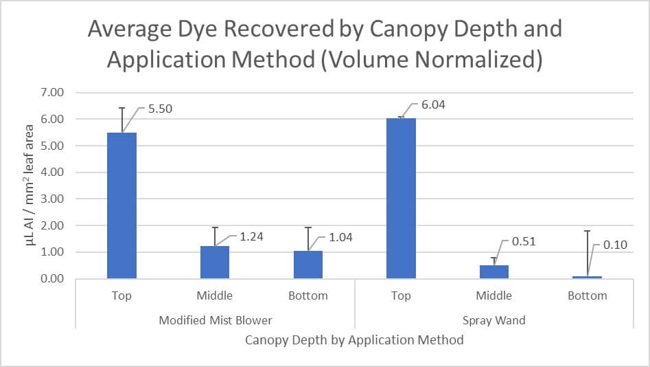
As mentioned previously, dye recovery was normalized by spray volume and leaf area for each condition. The results align with inferences made in the above image. Spray coverage can be highly variable which often leads to statistically insignificant results, but the mean-dye-recovered does demonstrate clear trends. The top of each canopy received a similar dose of dye for each condition. This comes as no surprise and is typical of any overhead application into a canopy. However, the air-assisted condition resulted in more than 2x the dye in the middle of the canopy and more than 10x the dye at the bottom compared to the conventional method.
When considered as a percentage of overall dye recovered, we see that the dye deposited was more uniform in the air-assisted condition. 16% of total dye recovered in mid-canopy in the air-assisted condition canopy versus 7% in the conventional condition. 13% at the bottom on the air-assisted condition versus 2% at the bottom of the conventional condition.
Conclusions
Based on this study, there is compelling reason to consider air-assisted applications in closed environments. Canopy penetration and coverage uniformity was improved in the air-assisted condition. In addition, there is potential for reduced water volumes, which mean less contaminated run-off and lower humidity levels in closed environments.
Future work would require a better-engineered sprayer than the prototype used here. Further, while improved coverage often improves spray efficacy, it is not always a direct correlation. An efficacy study comparing crop damage and pest counts should be performed to confirm that this method of application represents a positive return on investment.
This research was performed with Dr. Sarah Jandricic, OMAFRA Greenhouse Floriculture IPM Specialist. Thanks to Schenk Farms and Greenhouses Co. for collaborating in the study.