I’d been pestering Dan Petker to let me come along as he and his father Paul applied 28% UAN to the winter wheat on their family farm in Port Rowan, Ontario.
Me: “Today?”
Dan: “Nope – Wheat’s not at the right stage.”
Me: “Today?”
Dan: “Nope – Rain in the forecast.”
Me: “Today?”
Dan: “We’ll see if the ground can hold a full sprayer. I’ll let you know.”
April 26th, 8:00 am
My first lesson was a reminder that farming requires a lot of advance planning and preparation because ultimately, it’s opportunistic. The Petkers were toeing the start line as they focused on weather forecasts, crop staging and field conditions. As soon as they determined that the wheat in the tram lines would bounce back rather than get mashed into the soil, they were ready to roll. I suppose I was opportunistic as well because as soon as I got the thumbs-up I dropped everything and raced to their farm.
10:30 am
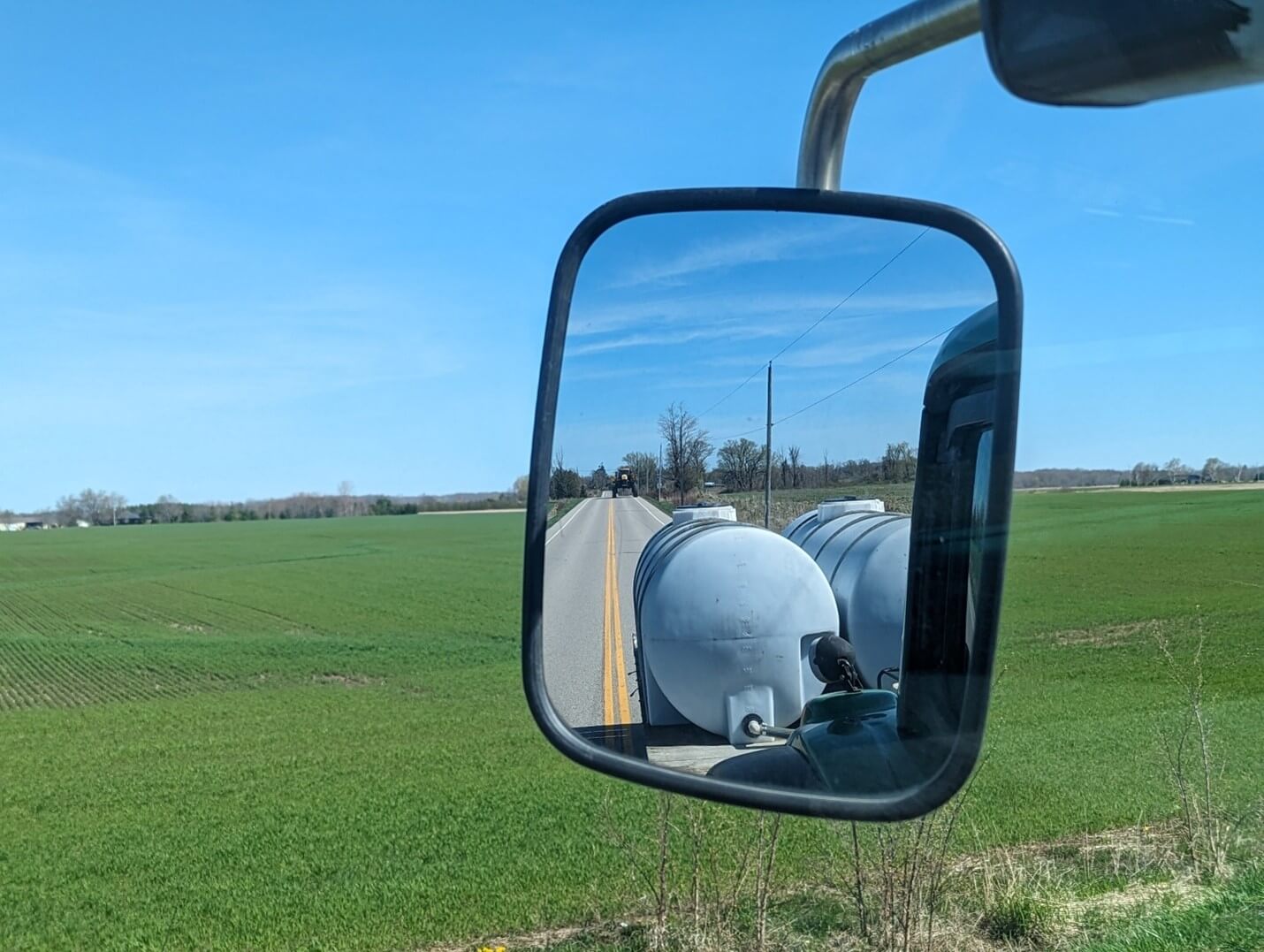
When I arrived, I found Dan filling their tender wagon in the yard. All their farm inputs are stored in their chemical shed, including 27,000 gallons of 28% UAN. The wagon had two, 1,000 gallon tanks which Dan was filling from a 2” line. He said that as the season progressed, they would move up to faster fills by swapping to a 3” line. They weren’t in that kind of rush today and he didn’t want to have to lug the heavier line around if he didn’t need to. Fair enough. At that point Paul radioed from the sprayer to tell Dan he was ready for his first refill.


As we drove to meet Paul, I learned that the goal was to spray two fields totaling 200 acres. A single, 1,000 gallon tankful would cover 20 acres. Dan noted that these soils were a loamy silt and clay mix that held nitrogen very well. On sandier soils, farmers often choose to split the application where a smaller amount is applied earlier in the season and the remainder later, but Dan said it never paid dividends on these fields. Of course, that reasoning may have been moot since it was such a wet spring; They couldn’t get out earlier even if they wanted to.
The two fields were within a 5 km radius from the yard, so nothing was more than 10 minutes away. The county roads were narrow, but throughout they day I saw that the locals knew how to share the road with farm equipment; lots of polite waves and no one risked their necks trying to pass. Good to see.

10:40 am
We pulled up alongside the sprayer and Dan started filling as I greeted Paul, who’d I’d ride with for the rest of the day. We were using their John Deere R4038 equipped with Pentair Hypro six-stream fertilizer nozzles (FC-ESI-11015’s) on 15” centres. The Petkers used 06’s the year before and found they had to drive too slowly, so investing in these larger nozzles was a productivity booster.

While filling, they both watched the sight gauge on the side of the sprayer. I asked why they didn’t use a flowmeter and they said it could be off by +/- 10 gallons, so if the sprayer was level, the sight gauge told them what they needed to know.
10:50
I joined Paul in the cab and we drove into the field. Paul pointed out the pink field boundary on the monitor and grimaced at the rounded corners that were established during planting. He wanted to reset the A-B lines and square off those corners. His reasoning was to ensure weeds didn’t grow in the margins and affect yield. However, he also said it looked terrible and I got the impression this was as much about pride in a job well done as it was yield.
We backed into the corner. Paul explained that the rate controller “hunts” a little as the sprayer speeds up over the first few meters and wouldn’t apply a full or consistent rate. By temporarily disengaging it until we got up to speed, we would avoid the weed escapes common to field corners. We’d be applying a slightly higher rate than required for those first few meters, but it was the lesser of two evils.

He set the first pass using GPS: “Got-Paul-Steering” and I watched as the breakaway section started snagging the treeline on the edge of the field. I asked if that was a problem and he replied that he was driving slowly, and it didn’t bother anything. It was important to get those margins and the trees were always growing and dropping branches, so hits were inevitable.
Soon we were back in the hands of GPS-guided autosteer and rate control and moving at a respectable 12 mph. 20 acres later we’d sprayed the 1,000 gallons and were headed back to meet Dan for a refill. On the way we noticed a triangular area that we missed while I was distracting Paul with questions. He said we’d double back later and let sectional control take care of it. Paul loved sectional control.
11:30
Soon Dan was empty, and we were full, so we got right back at it. I wouldn’t describe the field as hilly, but it was far from flat. On occasions where the sprayer dipped significantly, one side of the boom would sometimes kiss the ground while the other hung precipitously in the air. We had the boom height set to about 36” but Paul was manually raising each side if the boom got too close. You can forget the fantasy of sitting back and letting the machine do all the work; It certainly wasn’t the case, here.

Slower travel speed and a reasonably-low boom are the best practice for crop protection sprays. However, streamer nozzles don’t form droplets and overlap was maintained, so I wasn’t worried about our lively boom causing drift or coverage uniformity concerns. I was, however, increasingly focused on my lower back and teeth. The buddy-seat didn’t have the padding or air-ride suspension Paul was enjoying.
When we hit level ground again, I began to appreciate the process of passing back and forth over a field. It was satisfying to watch the sprayer icon on the monitor filling the screen with blue as we covered ground. Like the old-school, low-res, 1980’s video games that ate all my hard-earned quarters. Then we were empty again and it was time to go beg for more quarters.

11:46
Dan was busy so we drove back to the yard rather than wait for tender. There was a Rogator on the road ahead of us and Paul pointed out the muck it was flinging from the tires. A quick peek behind us showed we weren’t tracking mud. Paul said it was because of their soil management practices – no-till left the fields better able to weather droughts and absorb rains. The Rogator was operating in fields that employed deep tillage and were full of standing water and now, muddy tire ruts. Paul pointed out a few such fields as we drove, and I could soon see for myself which fields were managed by the Petkers and which were not. In fact, I only saw one puddle of standing water in their fields that day when all around us were shallow swimming pools.

12:15
We filled, drove back to the field, and picked up where we left off. Paul noted they had to plant their wheat a little later than they would have liked because they were delayed getting the beans off. Despite that, he was very happy with the stand we were fertilizing. We were able to have this conversation because Paul (like Dan) did not listen to music or podcasts in the sprayer. He said it helped him focus and that he liked the peace. I think being alone with my thoughts all day would have driven me around the bend. And then we were empty again, so back to the yard.

12:47
We filled, drove back, engaged the A-B line, and started the last section of this field. I asked about sprayer sanitation. UAN is notoriously caustic and can cause compatibility issues with some products, so I wanted to know how diligent they were about rinsing or cleaning (two different things). Paul agreed that it was messy stuff and it got all over the sprayer. So, at the end of the day, they would perform a thorough rinse of the plumbing before washing the exterior out behind their equipment shop. We finished with 300 gallons left in the tank, so we elected to head over to the second field.
1:10
At field number two, Paul changed fields on the monitor and grumbled about the round corners on the boundary. He pointed out that the edge of this field wasn’t straight – it contoured along a wavy treeline. Paul briefly disengaged rate control, set the “A” point and started driving manually again, hugging the treeline and dipping in and out using Got-Paul-Steering until we’d cleared the trees. Now that the field boundary was straight, he erased the “A” point and set a new one before later setting the “B”. He looked over at me, anticipating my question, but I’d already guessed that Paul didn’t want to repeat that wavy line on every subsequent row. Instead, we’d now run parallel to a straight A-B line and let sectional control handle the overlaps on our twisty start. That earned me an approving smile. And to add to that feeling of pride, our tank emptied exactly at the end of that first row. Perfect.

1:27
Back at the yard for our refill, I thought about how long our previous fill times were compared to now. From this second field it was 10 minutes on the road, 10 minutes to fill, and 10 minutes back, so 30 minutes compared to maybe 15 for the first field. Longer than I thought it would be. At 1:48 we were back and spraying again and I was beginning to notice how technical this field was. We performed a number of three-point turns in order to back into corners while the monitor alternated between happy chirps and stern alarms as we passed over A-B lines. Then we were empty, so back we went for more.
2:41
To continue to video game metaphor, this field was an advanced level and the Big Boss was coming. Not only was the shape odd, but it had chain link fences, posts, more trees, a water course, and they stored some farm equipment on one part of it. Paul calmly negotiated all these obstacles with stops, starts, boom adjustments (either height changes or partial folds), and then, shockingly, asked me to drive.
Paul: “Line up the tracks.”
Me: “I’m trying.”
Paul: “Do not try or you won’t get it right. Do!”
Me: “…what!?”

As a card-carrying Star Wars fan, I thought Paul was teasing me. His Yoda impression was perfect. I asked if he’d seen Star Wars and he replied that he was vaguely aware of it. So, he was being sincere, and I relaxed knowing I was in good hands. I even negotiated a few turns under his tutelage. But I confess I was relieved when the hydrostatic lightsaber was back in his capable hands.

3:04
Empty. Drive. Fill. Drive. Spray at 3:43. The last section was quick and easy and once we’d finished, we headed to their equipment shop to find Dan waiting. Dan pointed out the nitrogen all over the sprayer and reinforced Paul’s assertion that they’d rinse it out and wash the exterior off later that evening.

He drove me back to the yard so I could retrieve my car and we said our goodbyes. As I was headed home, I happened to pass their equipment shop where I saw Paul, a man in his mid 70’s that hadn’t stopped to eat and had been spraying all day, hard at it washing off the exterior. Wow.
Take Homes
I’m guilty of over-emphasizing the fill-time aspect of spraying because that’s the biggest time-suck on productivity. However, some tank mixes (e.g. SC’s) don’t appreciate being rushed, and while time is always pressing, there are those occasions where it isn’t mission-critical. Fill-time never came up on this job. There were, however, other aspects that deserved attention.
In the case of applying UAN to winter wheat on these irregularly shaped home-farm fields, it was more important to be attentive and manually adjust sprayer settings to fit the moment rather than always trust in the technology. Granted, the technology (namely rate control, boom leveling and GPS sectional control) was brilliant once we’d finished the headlands and dealt with any obstacles and topographical challenges.
I also appreciated that this family has been farming for many years. Dan and his father had a practiced rhythm that made it look easier than it actually was. Equipment was prepared, decisions were made, and everything was in place well ahead of the application. That included how they managed their soil and knowing how their fields responded to nitrogen. They communicated well, using digital records and redundant written notes to ensure everything was coordinated and going to plan, and that good planning made for a good day.
And it was a good day.