Any description of airblast sprayer start-up must, contextually, make assumptions on how it was winterized for long-term storage. This cyclic relationship is why I use a chicken-and-egg title slide when giving this presentation.
Answer: It was the rooster.
The inability to describe one process without the other is further complicated by the possibility that the sprayer is brand new and was therefore never winterized. So, what follows is an attempt at a logical sequence of pre-season maintenance activities to restore a winterized sprayer, or initiate a new sprayer.
New Equipment
If this is a new sprayer, you have an opportunity to perform some preventative maintenance.
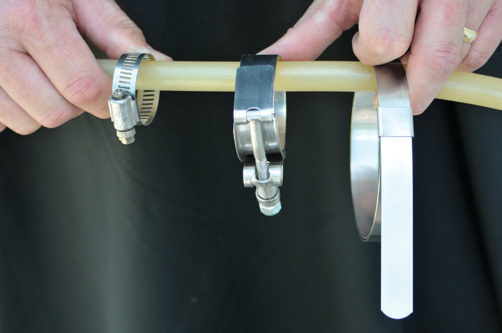
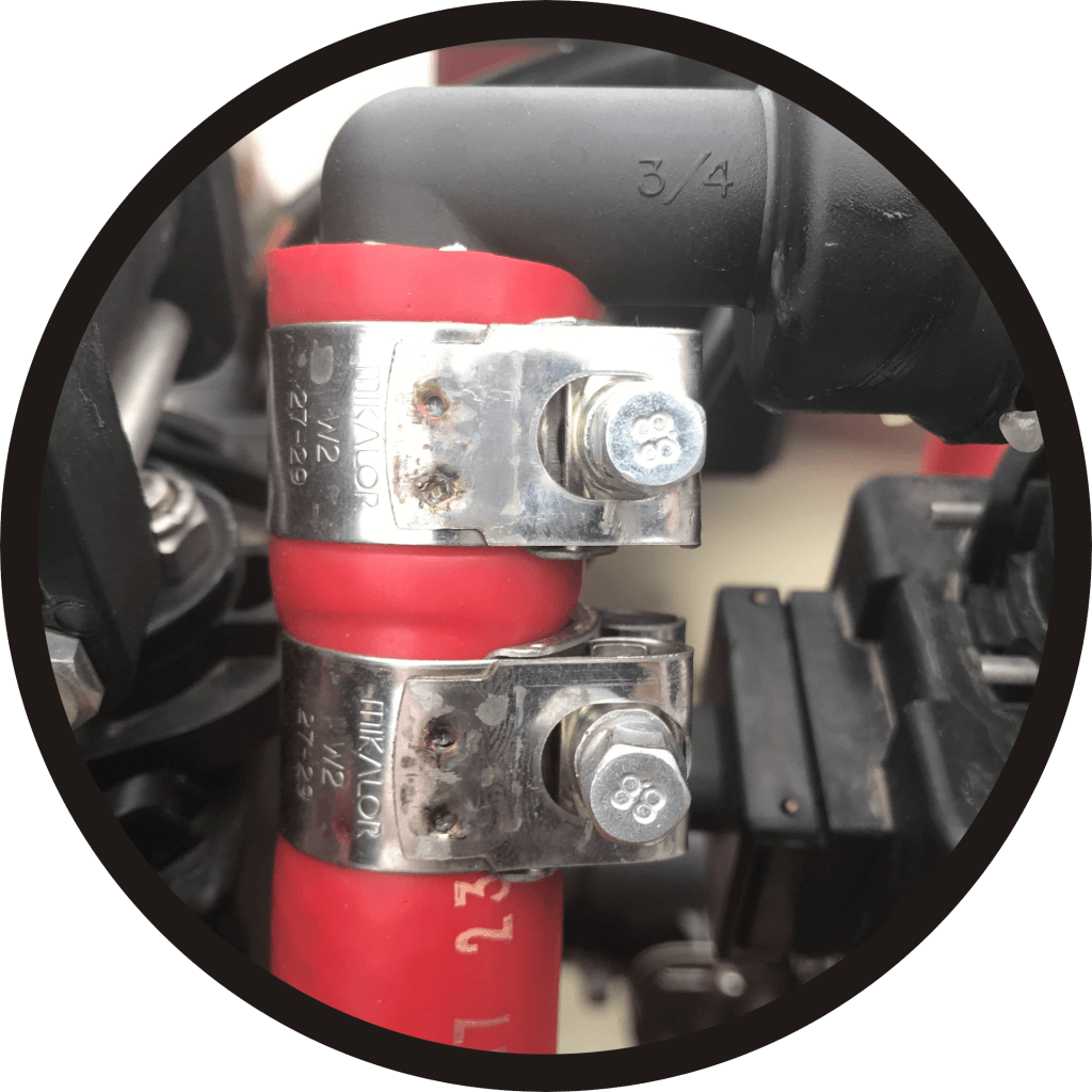
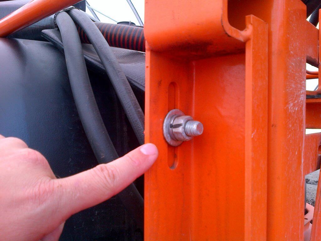
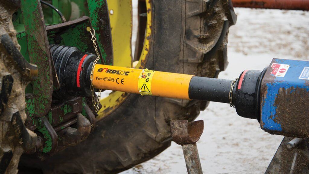
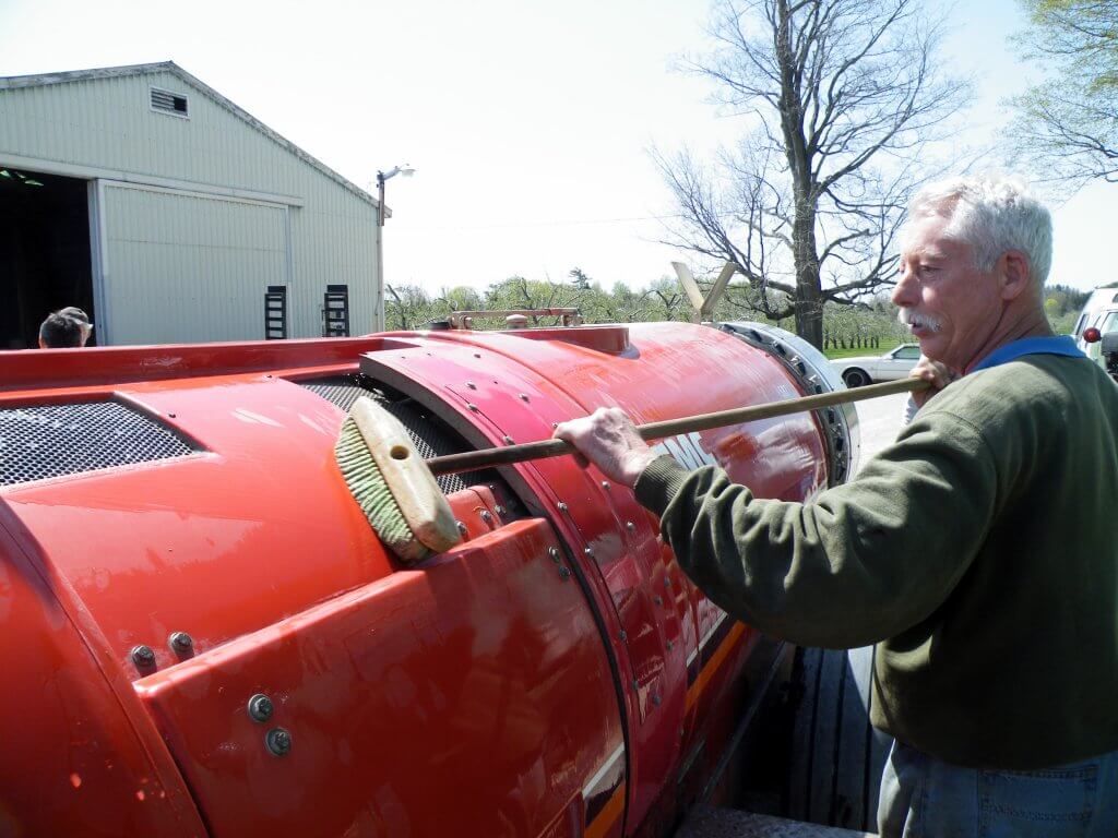
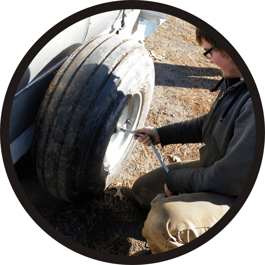
Loosen, lubricate and re-tighten clamps. Always back gears off before tightening to avoid stretching them. (Image from Purdue Extension publication PPP-121: Preparing Spray Equipment for Winter Storage and Spring Startup)Use double clamps on pressurized lines for added safety. Wider clamps are better and T-bolt clamps are better than worm-gear.Put thread release on bolts and re-tighten with a torque wrench (not an impact tool). Use a paint pen to mark nut, washer and bolt for future visual checks. This is called a “Witness Mark”.Protect hoses and wires at rub points. Follow hoses and with a paint pen, number the hose-ends and connections for future reference.Using a new tractor? You may have to re-calibrate to account for different gear ratios. When hitching a new sprayer, note that the distance from the ball on the drawbar hitch to the tip of the PTO should be ~14″. Don’t exceed maximum working angles for PTO shafts (usually <25 degrees). If your tractor or implement manufacturer says differently, go with that. And get it in writing.
Winterizing (Long-term storage)
If you are preparing the sprayer for long-term storage, follow the normal rinsing process, but don’t reinstall strainers and nozzles.
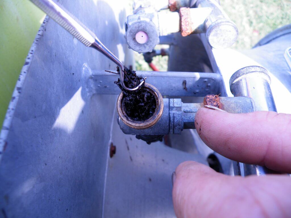
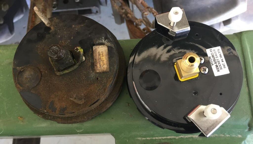
Look in the nozzle bodies for debris. Discard worn or broken nozzles.Soak, scrub, rinse and store nozzles and nozzle strainers. You may replace them once the sprayer is clean, but I prefer to store them separately since they have to come back off during start-up.
With the agitation on, circulate undiluted plumbing antifreeze (the sprayer already has 5-10 L (1.25-2.5 gallons) of water in the system from the decontamination process) for five minutes and drain it through the plumbing system (not the booms).
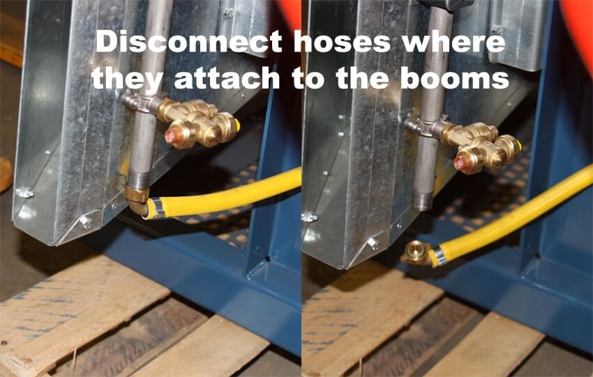
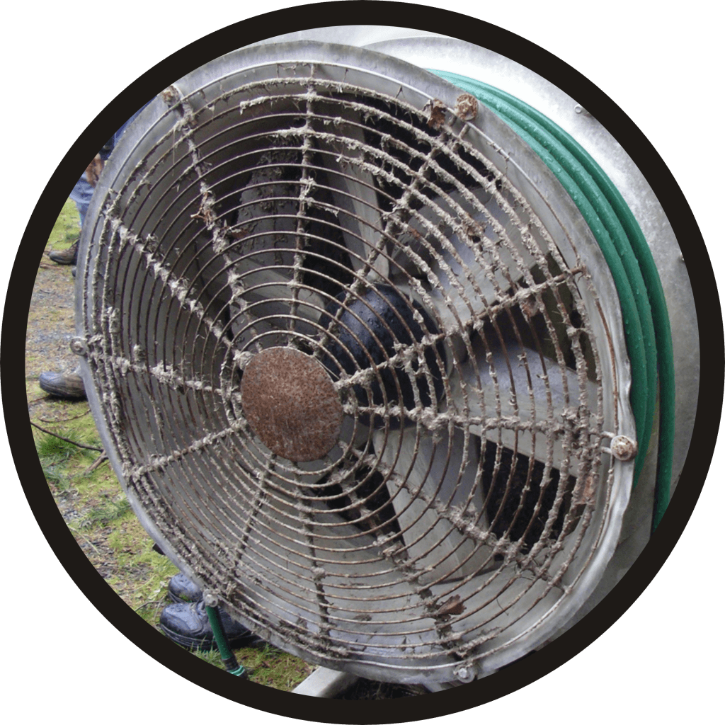
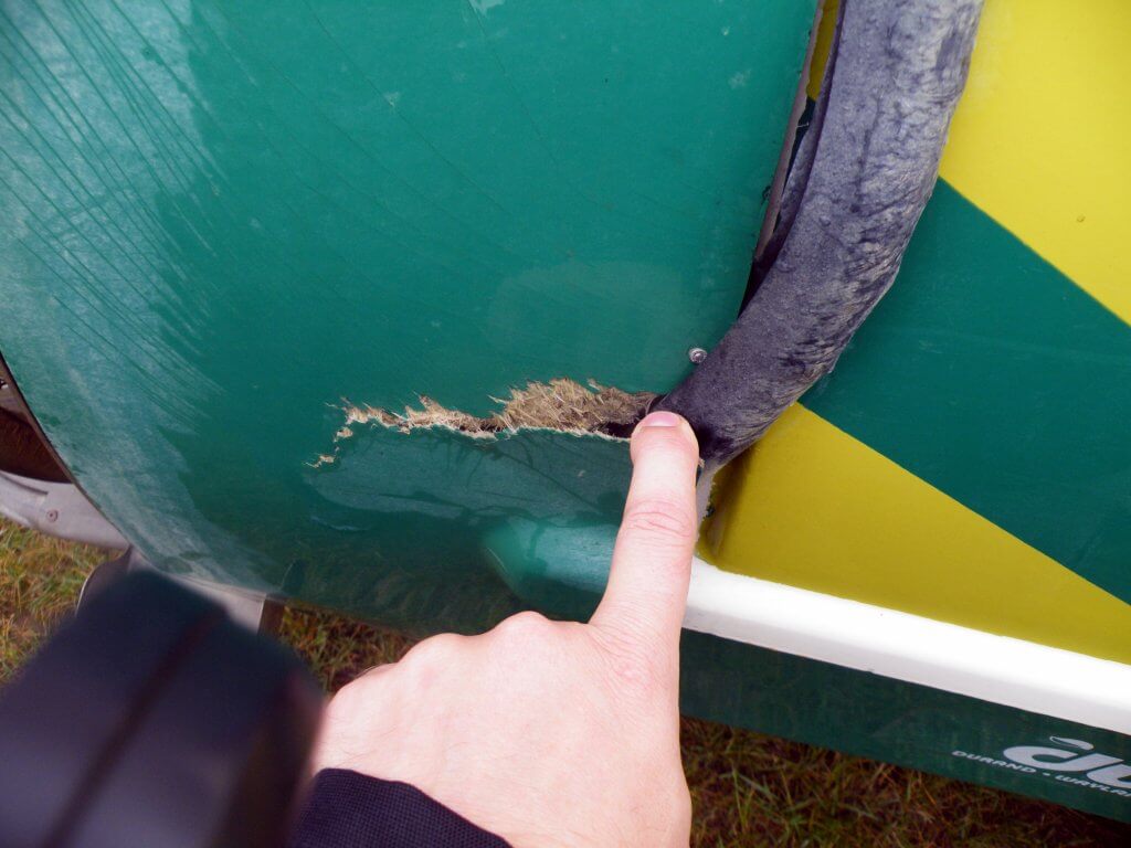
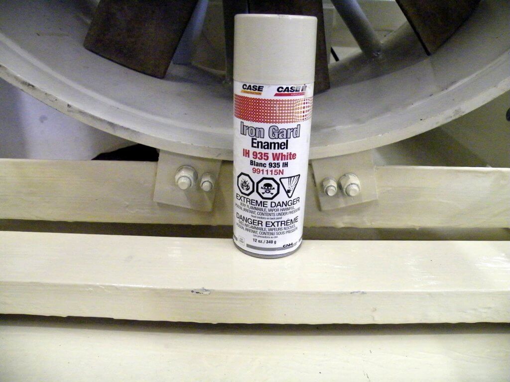
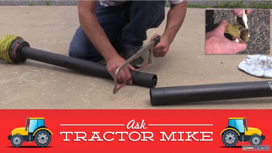
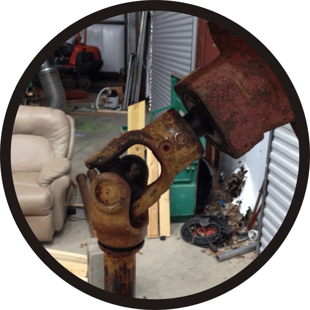
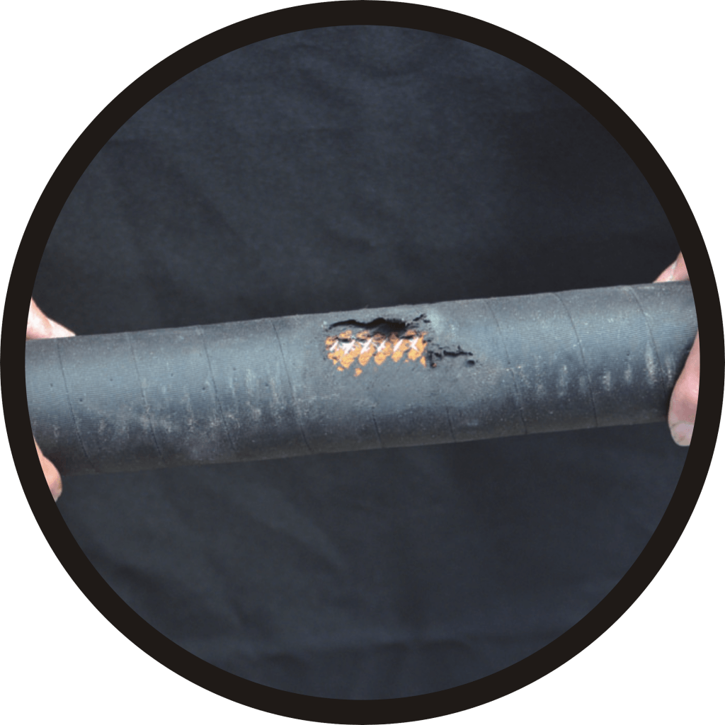
Disconnect hoses where they attach to the booms and drain as much liquid from the sprayer as possible. (Image from Munckhof Sprayers). Take the time to examine any hose fittings.Clean the sprayer (Triple rinse with a detergent) and scrub the exterior. Do not use pressure washers on bearings, fittings, pumps or any lubricated or moving parts.Examine fan blades for cracks, build-up or nicks that can cause imbalance. Replace (not just repair) punctured entrance grills.Don’t ignore tank damage. Poly tanks are prone to sun damage and cracks. Never climb into a tank to repair it. Quite often, replacement is the best option.Clean and inspect wheel assemblies. It’s best to do this during winterization to prevent bearing corrosion as the sprayer sits all winter.Remove any rust and repaint (or just touch up). Paint not only looks good, it protects.The excellent YouTube channel Ask Tractor Mike proposed storing the PTO shaft indoors in two pieces, and to cut away a portion of the interior guard to facilitate reassembly later on. Also, use a paint pen to mark the splines on the shaft for easier hook-up (see inset top-right of image).RV antifreeze is a 50% solution of antifreeze and water with a rust inhibitor. It should not cause phytotoxicity if sprayed or dumped, but be sure to dispose of it away from water sources during start-up. Turn the pump manually to get antifreeze throughout the system. Close the nozzle bodies, loosely fit the tank lid and store indoors. (Image from Purdue Extension publication PPP-121: Preparing Spray Equipment for Winter Storage and Spring Startup).
Spring Start-up
Most operators are guilty of neglecting their airblast sprayers and babying their tractors. Sprayers are precision tools that must be kept in good operating order to prevent costly breakdowns, improve their performance, and increase their lifespan.
Your car is serviced based on distance travelled. Your sprayer should receive regular maintenance based on working hours, per the manufacturer’s recommendations. Daily sprayer inspections are part of regular maintenance since the operator will (hopefully) find small problems before they become big problems.
Never assume your sprayers is ready to go right out of long-term storage. Parts seize, scale breaks away from surfaces, and small beasties sometimes choose to eat, or make their homes in, cozy sprayers.
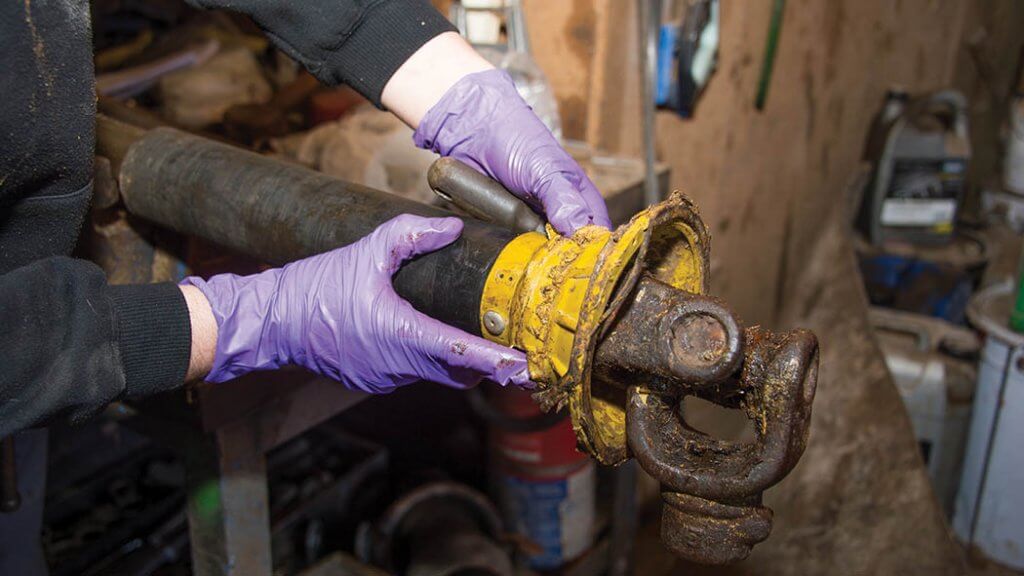
When planning spring start-up, never assume the winterized sprayer is ready for immediate hook-up. Expect a minimum half day per sprayer.Attempting to loosen or shift something that hasn’t moved in several months is risky. Pressure gauges snap off, fittings crack, welds break. Expect the unexpected and either have spare parts on hand, or a plan to get them quickly.Parts are most likely to seize during the first spray. Bearings and PTO universal joints, especially.Start-up is a good time to lubricate parts. Grease the guard ring bearing every 100 hours, the universal joint cross every 25 hours and the shaft and shear bolt regularly.Insects, birds and rodents eat, or make homes in, sprayers. Professional rodent bait/traps, steel wool and peppermint oil/gel are possible solutions.Check belt tension, alignment and wear. (Image from Purdue Extension publication PPP-121: Preparing Spray Equipment for Winter Storage and Spring Startup).
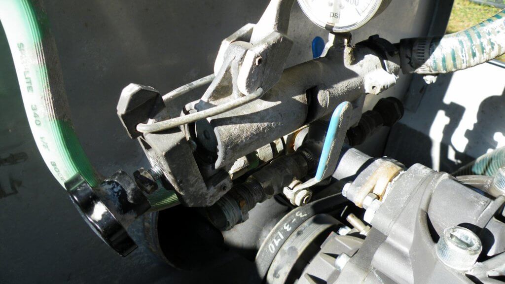
Pump specific maintenance is beyond the scope of this article. Hypro recommends changing oil after 40 hours of break-in operation and every 500 hours after that. The diaphragms should be replaced every 1,000 hours. Generally speaking, EPDM (black) diaphragms are a better choice for airblast sprayers, while the Desmopan (amber) diaphragms are really for lawn care sprayers.
Pump maintenance is beyond this article, but change the oil every 500 hr or 3 months. Use a paint pen to write on the pump what type of oil it requires, and then date the filters. Note the “winterized” sticker.
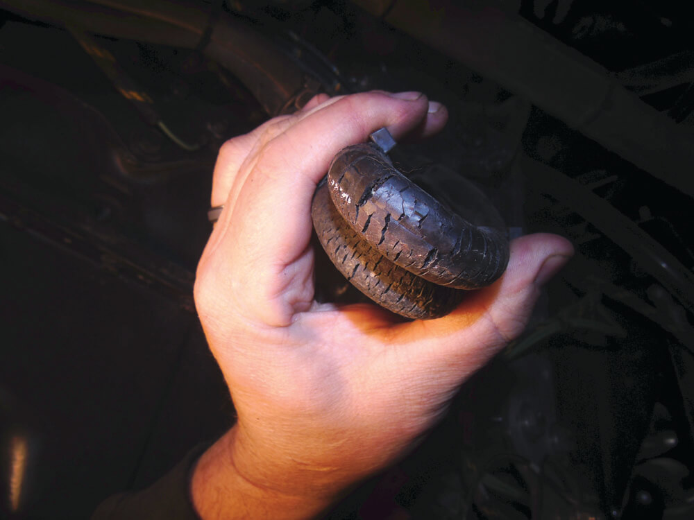
At minimum, check the tire pressure. Hard tires drive faster, but leave compacted ruts. Soft tires drive slower, but disperse weight better. Airblast sprayer wheel assemblies should be cleaned and inspected as part of regular annual maintenance. Wheel bearing maintenance before long-term storage may prevent water from corroding the bearings.
Ensure tire pressure matches the ideal stamped on the tire. Or, if using less pressure to avoid spring soil compaction, ensure both tires have the same pressure.
The relief valve on your sprayer should always be in the bypass position during start-up. If your gauge spikes then the gauge may always read high afterwards and should be replaced.
A reminder to always set the relief valve to the bypass position when starting up the sprayer. This is one reason why pressure gauges spike and can eventually fail.
Replacing leaking, opaque or inaccurate gauges improves sprayer performance. Be sure to use the oil-filled variety of gauge to eliminate a bouncing needle. You can also get suppressors that fit between the gauge and sprayer to prevent pulsing. Consult the article on testing airblast pressure gauge reliability.
Use a wrench to turn gauges at the nut. Don’t twist them by hand holding the face. Ensure they are not opaque, leaking, plugged or resting above the zero pin.
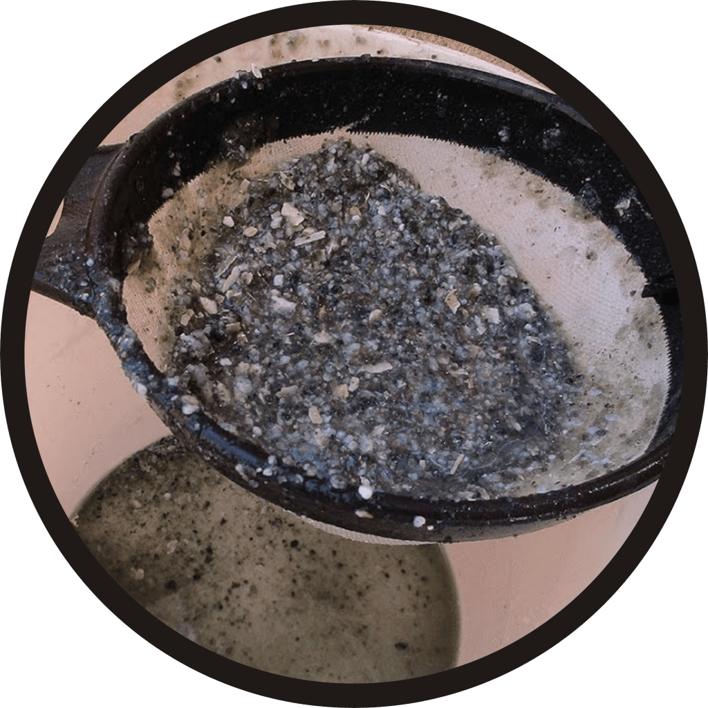
Many spray materials do not mix well and one of the common causes of uneven application is poor agitation. If you find deposits at the sump in the bottom of the sprayer after an application, your agitation is insufficient. For mechanical agitators, check for propeller wear and ensure paddles are secure on the agitator shaft. Learn more about agitation here.
If the agitator shaft is leaking a little, tighten the packing. The packing gland is a common source of leaks. Keep it properly greased. If a leak occurs you can usually repair it by tightening the bolts on the packing gland by ½ a turn, but if that doesn’t work you may have to remove and repack (or replace) it.
On sprayers with mechanical agitators, look for prop wear and loose or damaged paddles. Fill the sprayer with water and looks for tank leaks. Tighten the bolts 1/2 turn if the packing gland on the agitator shaft is leaking. You may have to remove and repack the gland if the leak persists.Look for signs of hose wear and examine the sprayer for leaks while under pressure. Be careful when pressurizing the sprayer for the first time in the spring; this is when lines are likely to come loose or burst. (Image from Purdue Extension publication PPP-121: Preparing Spray Equipment for Winter Storage and Spring Startup).Minerals chelate (i.e. scale) more readily on stainless steel than plastic tanks. In either case, the first tank of water and leftover antifreeze should be sprayed from the nozzle bodies with no line or nozzle strainers, and no nozzles. Replace them once the tank is sprayed out.
The last step is calibrating the sprayer, and that process really depends on your definition. If the preceding steps conflict with those of the manufacturer’s, always follow the manufacturer’s. Do this for reasons of safety and to preserve any warranty.
Thanks to Fred Whitford (Purdue University), Gail Amos and Mark Ledebuhr (Application Insight LLC) for reviewing the content of this article and for their helpful edits.
In the summer of 2024, six Ontario vineyards participated in an authorized herbicide trial. The objective was to assess efficacy as well as determine if the product fit the timing for seasonal weed and sucker management. If successful, it could replace the expensive and time-consuming manual labour required to remove suckers.
Each vineyard applied the same rate, at similar times, employing optimal sprayer settings. A few weeks after application, the researchers and registrant toured the vineyards. They were pleased with how quickly and effectively the product worked on both targets at all six locations. However, one vineyard reported visual injury on a sloped region of their operation.
This raised two questions:
Assuming the cause was drift, and not direct overspray, why did it only happen in a specific region of a single vineyard?
Whether drift or overspray, what is the potential for the applied rate to cause injury?
The vineyard manager and sprayer operator investigated the application equipment and found no problems with how the sprayer was calibrated or operated. Further, the nearby weather stations recorded reasonable environmental conditions. So, that seemed to discount accidental overspray and wind-borne drift.
Then we considered the topography. The level portion of the vineyard appeared undamaged, but as it began to slope downhill, we saw damage on leaves and shoots in the bottom half of the canopy. It was almost as if a stratum of herbicide stayed level as the ground fell away. We discussed temperature inversions, volatility, and sprayer wake, but nothing fit.
Then we stepped back and found ourselves looking up at the Niagara Escarpment. The Escarpment is a long cliff formed by erosion, separating the higher, level ground from where we stood below. And then we had an idea: Could the product have been lifted into contact with the canopy by a Katabatic wind?
The theory
On clear nights with calm winds, the ground cools rapidly. Air in contact with the colder ground cools by conducting heat to the ground and by radiating upwards. When this cooling process occurs along mountain slopes, or on top of a plateau, the cooling air becomes colder and denser, causing it flow downslope like water. Perhaps a layer of relatively cool Katabatic wind off the escarpment slid under the warmer layer of air in the downslope portion of the vineyard. And, perhaps, any product still suspended in the air was lifted upwards into contact with the grape canopy.
Cold air (blue) slides under a warmer layer of air (orange) that carries traces of herbicide in the form of Very Fine, suspended droplets. It is lifted into contact with the lower portions of the grape panels.
Even the coarsest hydraulic nozzle produces a population of driftable fines. These fines take a long time to fall, and some are essentially buoyant. In the following histograms, we see actual data from a nozzle rated between Medium and Coarse. The operators actually used an air-induction nozzle with a much coarser spray quality, but we’re using this data set as a worst-case scenario example. If we divide the volume produced into its constituent droplet sizes, we see that most of the volume is comprised of droplets between 150 and 250 microns.
However, droplet diameter shares a cubic relationship with volume. If we plot that same volume by number of droplets, we see the majority are between 18 and 74 microns in diameter. These very small droplets would fall so slowly that any atmospheric disturbance would displace them. Depending on the crop’s sensitivity to the herbicide, they might carry sufficient active ingredient to cause injury, assuming they didn’t evaporate to the point that they were no longer biologically active.
There are a lot of assumptions in this theory, and perhaps it’s far fetched, but it was the best we could figure. So, if those droplets were lifted into contact with the canopy, were they capable of causing injury? To find out, we conducted a simple, non-replicated bioassay.
The bioassay
On the morning of July 12, we filled a spray bottle with 50% of the field-rate (including 1% v/v MSO) and set the nozzle to the finest setting. We applied a single spritz about mid-way up the canopy of the same Riesling grapes on a VSP flat cane training system. We did this on the upwind side on both older (lower canopy) and newer growth (upper canopy). Then we performed a series of serial dilutions, halving the concentration each time, and repeating the application.
Our hope was to see a subtle response curve when we plotted concentration against tissue damage. Perhaps we’d even see a different curve for older versus newer tissue.
The vineyard manager photographed and recorded observations on an approximately weekly schedule, with a gap in observations between weeks three and six. The following images show the results of a ½ dose treatment, and a 1/16 dose treatment tracked during that period.
The results
We observed the following:
Fruit, foliage, and shoots were injured at all doses by three days after application.
Initial injury remained stable; no secondary injury was observed.
The degree of injury at the lowest dose was significantly more severe than the injury observed following the original May 31st application.
Regular vineyard operations, such as mechanical leaf removal in the fruiting zone and hedging, removed some of the damaged leaves and shoots.
The study did not include an assessment of harvest quality.
This was severe injury, even at the lowest rate. When compared to another herbicide commonly used for perennial weed control (e.g. Ignite SN – glufosinate ammonium) the injury we saw manifested very quickly.
Recently, researchers at Cornell have been exploring the herbicide we used in this study in perennial weed and sucker control in apple orchards. They did not experience any drift issues and found it to be effective between 90-180 ml/ha (0.5-1 oz/ac) (personal communication). That’s ~4x less than the rate proposed for registration in Canada, and it suggests the herbicide in question was certainly capable of causing the damage at very low concentrations.
Ultimately, we can’t be certain how the initial off-target damage occurred, but we were able to evaluate damage potential using a rough-and-simple bioassay that any grower can try. In unusual cases of drift it’s important to know if the product we suspect is even capable of causing the damage. A simple evaluation using serial dilution and a squirt bottle can tell us if we need to look more closely, or look somewhere else to explain injury.
Thanks to Kristen Obeid, OMAFA Weed Specialist (Horticulture) and Josh Aitken, Vineyard Manager of Cave Spring Vineyard for their contributions to this work.
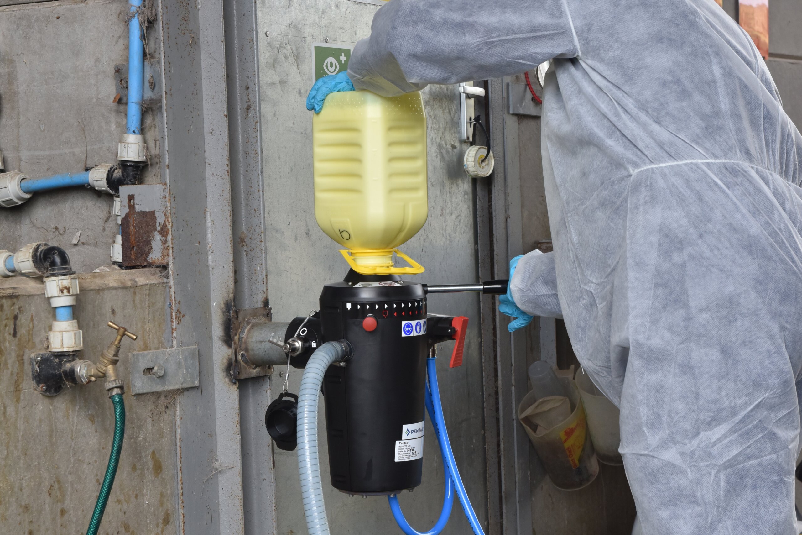
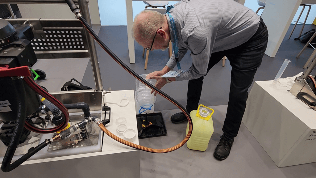
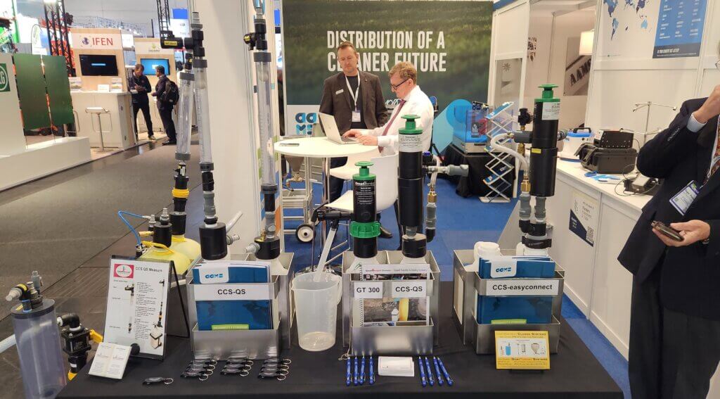
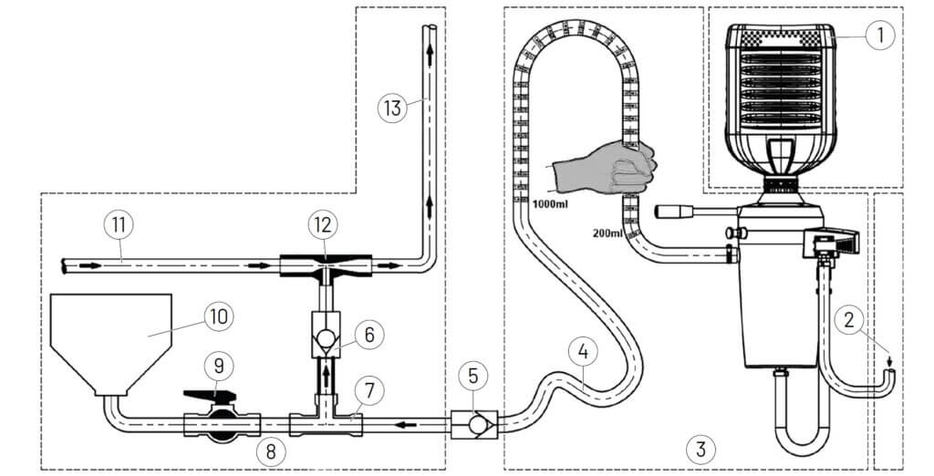
Closed Transfer Systems (CTS) permit the direct transfer of pesticides from container to sprayer while isolating the process from the operator and the environment. Similar systems are already used with bulk pesticide containers and in other industries to dispense a wide range of liquids from household products to industrial chemicals. In the case of small-volume containers (e.g., up to 20 L), these systems include an integrated container rinsing function.
The UK’s Iain Robertson testing Pentair’s Cleanload Nexus Coupler
CTS are comprised of two parts: The Cap (or Adaptor) and the Coupler. The CTS cap is either pre-fitted on the pesticide container, or the user must remove and replace the existing, non-CTS cap with an adaptor. Generically, the container is then locked into the coupler, and a valve in the cap or adaptor opens to permit chemical to be drawn out. If a partial amount is required, the valve can be closed to re-seal the container for safe removal, and the coupler and lines can then be rinsed. If the full amount is required, then the container is also rinsed prior to removal.
Regulatory Requirements: Canada
Canada’s Pest Management Regulatory Agency (PMRA) considers the requirement for closed transfer when products go through their natural re-evaluation cycle. They define it as follows:
“A closed system means removing a pesticide from its original container, rinsing, mixing, diluting, and transferring the pesticide through connecting hoses and couplings that prevent exposure to the pesticide.”
The requirement is primarily a means of reducing operator exposure and point-source contamination during filling, but can also be used to impose rate restrictions, or in response to reformulation. In recent years, several pesticides have had statements added to the labels regarding the requirement for a closed transfer system. They have stated that there have been three scenarios that they have included closed systems on labels:
The registrant requested closed systems be used in the occupational risk assessment.
Closed systems were required when triggered by the occupational risk assessment as a form of mitigation to reduce exposure to the mixer/loader. This is the most common reason it gets added.
Closed systems were used in the specific exposure study submitted to PMRA that was used in the risk assessment.
As standardized language is developed, Canadian operators can expect to see statements that vary in their specificity, such as in the following two examples:
Product 1: “Requirement for additional personal protection equipment (PPE) and engineering controls when mixing/loading and applying to various crops.” Product 2: “Closed mixing/loading systems are required. A closed system means removing a pesticide from its original container, rinsing, mixing, diluting, and transferring the pesticide through connecting hoses, pipes, and couplings that are sufficiently tight to prevent exposure of any person to the pesticide or rinsing solution.”
Questions and concerns have been raised by registrants and growers as these changes have appeared on pesticides with particularly important actives. As of 2025:
Products with standard CTS label statement:
Lorox L Herbicide
Ethrel PGR
Dibrom Insecticide
Products that require CTS without standard label statement:
Bravo ZN Fungicide (bulk totes only, chlorothalonil in 10 L jugs does not require CTS)
Captan 480 SC and Captan L Fungicide (only if open cab AND exceeding a maximum L/day threshold)
Products that may require CTS but not clear on the label:
Sevin XLR Insecticide – “use a closed mixing system”
In some cases, registrants have avoided the requirement by splitting the label rate and promoting multiple applications to ensure rates do not reach the PMRA’s threshold for closed transfer. Another strategy is to remove small-volume formats and rely on Intermediate Bulk Containers (IBC or totes), which already employ closed transfer. If neither option is available, registrants may face expensive changes (which are currently unspecified) to their injection molding process. This is assuming North American small-volume container packers respond to emerging Canadian requirements.
Commercial horticultural and specialty crop growers (or field croppers with smaller acreages and diversified crops) are more likely to purchase pesticides in small-volume containers as opposed to a tote. For growers, the practical requirements for compliant closed transfer are not well understood. Most do not currently have CTS and feel a retrofit is overly burdensome (e.g. slow, expensive, complicated), incompatible with their equipment, or redundant with conventional PPE.
As Canadian agriculture comes to terms with these regulatory changes, the European experience offers valuable insight.
Regulatory Requirements: Europe
In Europe, reducing operator exposure and point source contamination during filling has long been a regulatory priority. Regulatory requirements for CTS are slated or already exist. The following dates are “fluid estimates” that will depend on the politics of each country. At the time of writing, the Netherlands are planning to make it compulsory on liquid formulations by 2025. Denmark will follow by 2024-25 and Belgium by 2026. The Czech Republic already stipulates about 12 separate products must be used in combination with CTS, and a blanket requirement is under discussion. In some cases, growers will be granted a three-year transition period before they must show that they have a capable CTS. Currently the UK doesn’t yet have any concrete targets, but they have been testing CTS since 2017 and their experiences have informed product development and the creation of international standards. According to a 2023 article in EI Operator, CropLife Europe stated that Europe is on track to make CTS available to all European farmers by 2030
Recycling
According to easyconnect (c. 2024), Germany is on the cusp of agreeing to accept both jugs and caps for shredding. Currently the caps are collected separately (if at all) because they aren’t typically rinsed. This is the same as in Canada.
Cap and foil collection awaiting disposal.
However, because the transfer systems also rinse the connection, the caps are down to the same 0.01% residue limit as the jugs, so as long as they’re dry, they’re both recyclable. Discussions are ongoing with France to make the same agreement.
ISO definitions of CTS
The 2021 publication of ISO 21191 has greatly facilitated CTS development. The standard defines what a CTS is and specifies the testing methods and compliance criteria for both operator and environment-related safety. Summarizing key points in the ISO:
The CTS shall
connect to containers and application equipment;
control flow and measuring of all or a part of the container content;
rinse the container into the application equipment;
flush the CTS equipment as well as the interface;
permit operation while using appropriate personal protection equipment specified on pesticide label and any associated operator’s manual;
have clearly labelled controls;
be designed to avoid any return of liquid to the clean water supply.
The CTS shall not
cause leakage when the device is connected to the mix tank or application equipment;
influence the circulation system of the connected application equipment;
allow the introduction of air that promotes foaming or reduces pump performance;
leave a residue level of more than 0.01% of the containers nominal volume following rinsing.
The ISO was reinforced by a 2023 Crop-Life Europe study that tested three systems applying for ISO certification. It demonstrated a more than 98% reduction in operator exposure (while using gloves) for the easyFlow M, GoatThroat, and Cleanload Nexus systems. These systems, and others, are described below.
Note: when using crop protection products, it remains a legal obligation for operators to wear the personal protection equipment indicated on the product label.
Commercial Systems
Pesticide container compatibility is fundamental to the success of any CTS design. There are exceptions, but many agrichemical companies in Europe and North America already employ a 63 mm screw cap for small-volume containers. According to the EPA (EPA 40 CFR Part 165 Subpart B), liquid agricultural pesticides in containers that are rigid and have capacities equal to or larger than 3 liters must have a screw cap either 63 or 38 mm in diameter and at least one thread revolution at 6 threads per inch. Depending on the CTS design, jugs may or may not require a tamper-proof foil. As of 2024, the first available jugs in the U.K. did not have foils.
The following systems are compatible with the 63 mm cap and are emerging as viable options at the time of writing. Some have been commercially available for several years and others are either new or still in development. Cost and availability will vary based on regional distribution and demand. Interested readers are advised to contact the manufacturer to confirm compatibility with their preferred products.
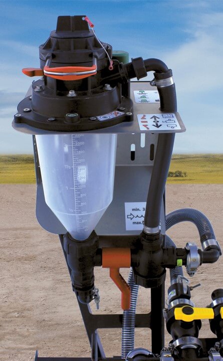
The easyFlow was developed with support from Bayer and has been available for more than 10 years. It requires the operator to remove the existing container cap and replace it with the easyFlow adaptor, which features a built-in knife that automatically cuts any foil seal. It is compatible with container sizes between 1 and 15 L. There are three versions of the easyFlow coupler.
easyFlow
The original easyFlow coupler installs directly to the sprayer tank. Once the pesticide container is joined (maximum 10 L format), product pours via gravity straight into the sprayer tank. The container can then be rinsed using an external water source (e.g. via a garden hose) with a min. ¾” diameter, anti backflow valve and water pressure between 3-6 bar.
easyFlow directly mounted on sprayer tank (image from FreeForm)
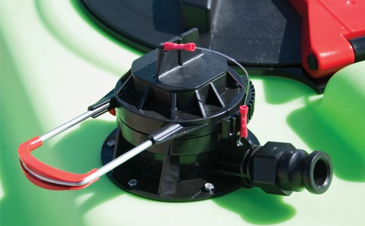
easyFlow M
The easyFlow M is a standalone coupler that supports containers over 10 L and permits dosing via an integrated measuring unit just below the mounting point. The measuring unit holds up to 2,250 ml with a minimum volume of 60 ml and graduations of 20 ml (50 ml over the 400 ml mark). Product transfer is achieved either by gravity, or by a pump (e.g. Teed to the suction side of the sprayer pump).
easyFlow M mounted on separate transfer station (image from FreeForm)
According to agrotop, a 5L container under suction took 2-2.5 minutes to empty and clean during the Croplife study. For reference, some operators claim they are able to drain and triple rinse in less than a minute using a traditional pour into an inductor. An operator in wheat aims to fill in 5-10 min depending and uses 5-10 jugs. On the other hand, CTS users have claimed a “hidden savings” from the overlap in operations where the product from one jug is still entering the system as another is being drained and a third is being prepared. AgroTop sells an optional vent spike called a “Chucker” that makes the process faster still, but penetrating the jug raises questions about ISO compliance.
Empty containers can then be rinsed before removal, or partial containers removed leaving the adaptor on the jug. While this unit can be mounted on the side of the sprayer, most UK farmers that have trialed this system opted to install it on a portable cart.
This system is still under development and information is limited. The easyFlow QF coupler reputedly has all the features of the M but is compatible with all manner of container and employs a 12 VDC supply to automatically meter the dose (starting from a minimum 1 L volume). The rinsing process is electronically automated as well.
Videos of the easyFlow systems in use can be seen hereand here. In the United states, these couplers are carried by Greenleaf Technologies. In Canada, it is also carried by FreeForm, a plastic molding company out of Saskatchewan.
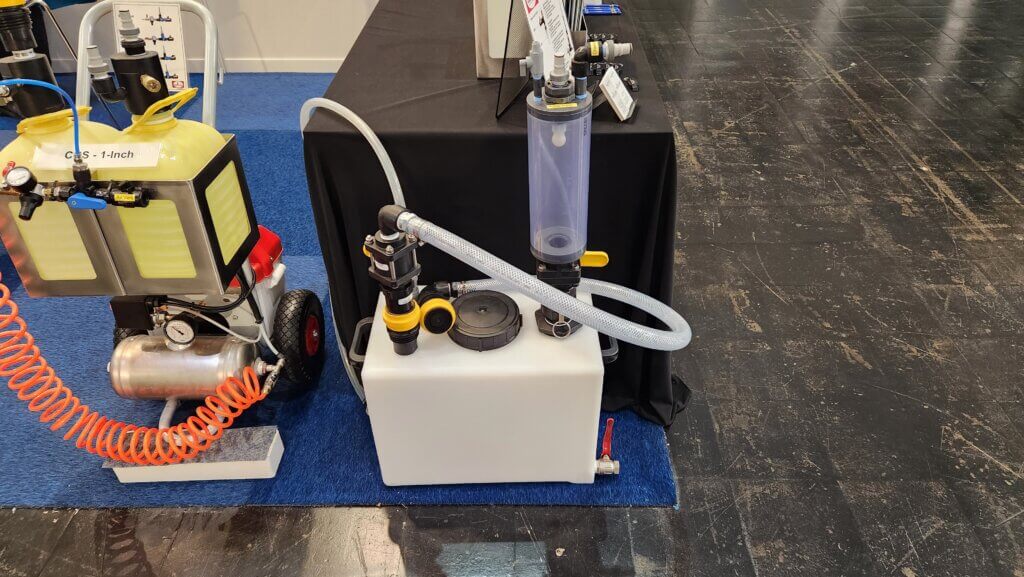
US-based GoatThroat has provided industrial liquid transfer solutions since 2001. Their CCS-8600 series requires the operator to remove the existing container cap and replace it with an adaptor with a siphon tube (which also pierces any foil). The container is then pressurized by a hand pump or compressor, forcing chemical into a measuring cylinder before it’s drawn into the sprayer. A clean water line then rinses the container (if emptied completely) and system before decoupling. The adapter can be left on containers if using partial volumes.
Comparatively, this system transfers and rinses more slowly than other small-format container systems and is entirely manual with multiple steps to transfer product. However, it now has a compressor option to replace manual pumping and it is highly customizable, making compatible with any container from a 1 L jug to a 1,000 L IBC tote. Further, its ability to transfer as little as 5 ml increments makes it a good option for small-acreage horticultural, specialty crop, and research farms where accurate partial loads are prioritized.
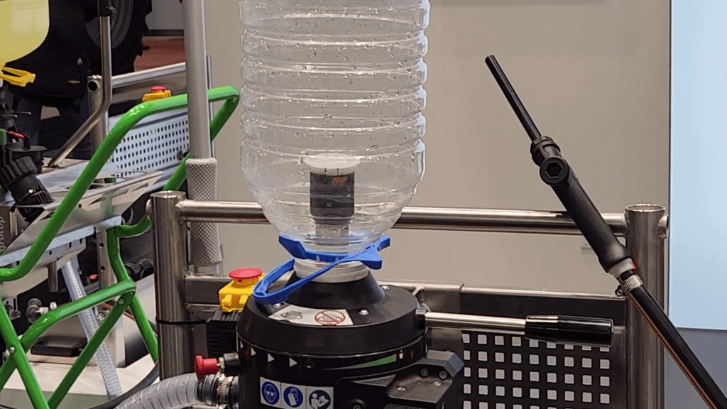
The easyconnect cap was originally developed by IPN Scholle with the support of BASF and is currently under development by Easy Cap and United Cap. It is compatible with container sizes between 1 and 15 L (possibly 20 L).
Because the cap is factory-fitted, it never has to be manually unscrewed or removed and works without requiring a tamper-proof foil. Its success is contingent on major agrochemical manufacturers agreeing to pre-fit it on their products. This has been facilitated by the easyconnect Working Group (ECWG), a consortium of ten major agrichemical companies, including those selling biological products and liquid fertilizers, that are supporting the European implementation of this format.
BASF displayed their compatible coupler, the ezi-connect at the 2023 Agritechnica in Hanover, Germany. Transfer requires the operator to snap off a dust cover, invert the container, and connect and lock it into the coupler. Another lever advances a probe and allows partial volumes to be dispensed via a vacuum generated by the hopper. Finally, a trigger controls rinsing water and undoing a catch allows the assembly to be rotated to improve cleaning without removing it.
Easyconnect will be factory installed on 1, 5 and 10 L containers in 2024. This will not be the entire portfolio from all agrichemical companies in the easy connect working group, but will represent a “significant amount” that will demonstrate commitment. In 2022, Syngenta released some information about their new jug format, the Evopac. In November 2024, Syngenta released this short video describing the design, which has the easyconnect cap and several features informed by sprayer operators to make it as safe and convenient as possible. The ezi-connect coupler will be launched in Europe in the 2025-2026 season.
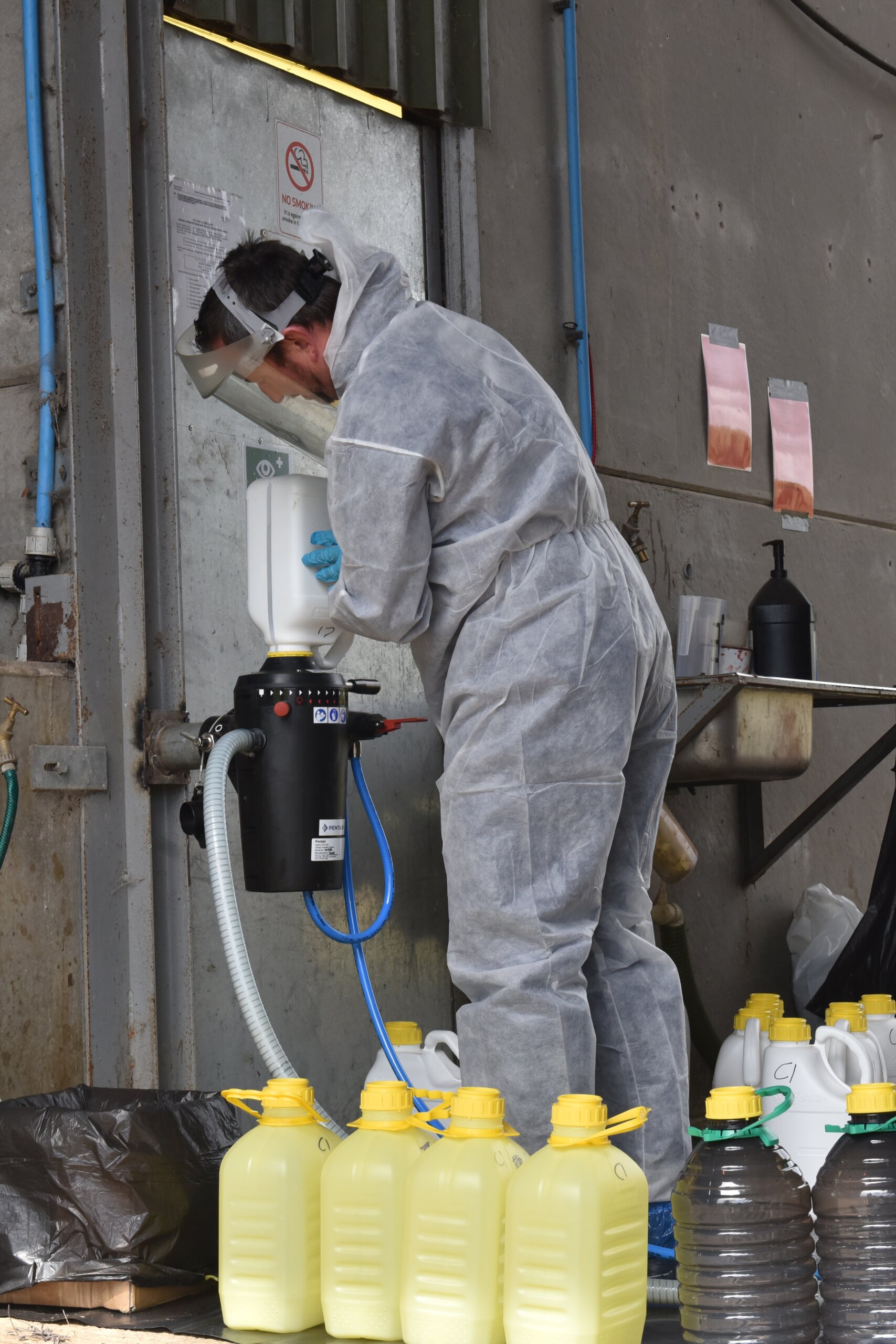
The Cleanload Nexus is a JKI-approved coupler designed for use with easyconnect caps on 1 to 15 L containers. The supplied 25 mm x 4 m suction hose can be connected by teeing it directly into the sprayer suction line ahead of the venturi (mounted to sprayer) or using a suitable dry-break coupler (mounted on a portable transfer station). The supplied 16 mm x 2.5 m rinse water hose connects to a clean rinse water source either on or off the sprayer.
The Cleanload Nexus in use
It is entirely mechanical and has just two manual controls. The first is a lever that locks the cap in place. Rotating the lever controls the emptying rate, which is between 0.5 and 1 L/sec at 4 bar, depending on liquid viscosity. The time to empty and rinse a 15 L container at 3.5 bar is about 2 minutes, and users have stated that this is as fast or faster than traditional pouring and rinsing methods.
For dosing, it currently relies on the operator using scale markings on the side of the pesticide container. It has been noted that the plunger mechanism displaces sufficient volume that it must be accounted for when reading graduations. Alternately, the calibrated suction hose connected to the sprayer can be used to assess larger volumes. The hose is, according to many, not a viable method for dosing and improvements are reputedly under development. Neither approach can achieve the ISO +/- 2.5% dosing accuracy, so Pentair has developed a dosing cylinder add-on that sits between the Cleanload Nexus and the sprayer and provides +/-1% accuracy (anticipated launch was in November 2023). A new measuring device, the Ezi-Connect VacTran Measure Unit by Wisdom Systems, was introduced in 2024 and is discussed in this article from EI OPerator.
Plumbing diagram for the Cleanload Nexus (from Pentair website).
While this video depicts 4 quarter-turns separated by 10-15 seconds rinses, practical application sees the simultaneous full rotation of the jug during a 30 second rinse. While the unit will rinse itself, some keep a dedicated jug full of clean water on hand and run that through the system last to ensure it’s left in a clean state. Note: operators say they only thoroughly rinse the cap when using a partial volume.
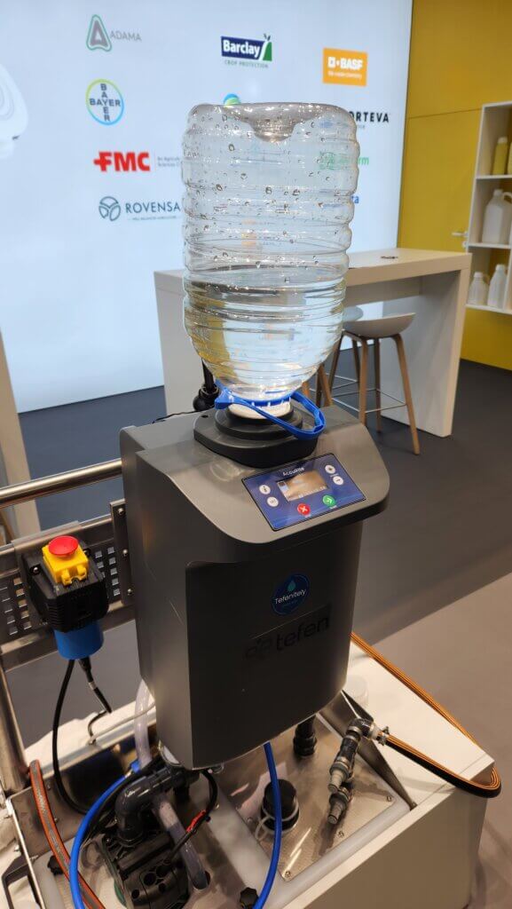
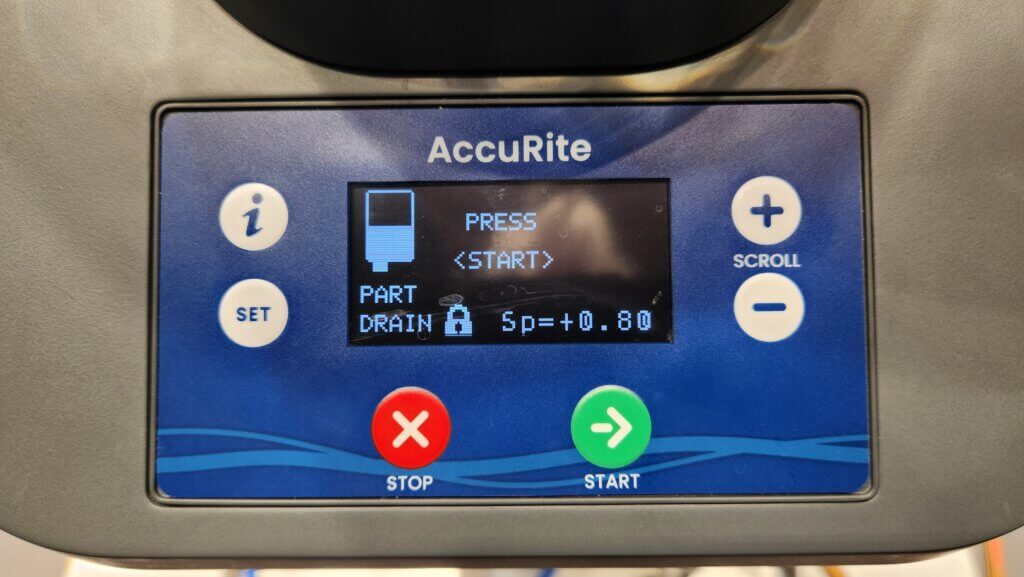
Israel’s Tefen has produced dosing pumps and flow products for many years and began field testing the AccuRite CTS coupler in 2022. With a single digital interface to operate the filling process and mobile capabilities for remote management and cloud-based record keeping (e.g., date, time and chemical usage). It is designed to work with the easyconnect cap on containers ranging from 1 to 20 L. This is slow compared with the ~60L/min. from the Pentair system, but Tefen is working to improve the speed.
Its diaphragm pump can deliver partial volumes at 0.1 L increments with an accuracy of +/- 2.5% of the smallest container used, and a minimum of 0.5 litres remaining in the container. Skip to the 1:50 mark to see the product reviewed (no English) in this video. In 2024, the following instructional video was released:
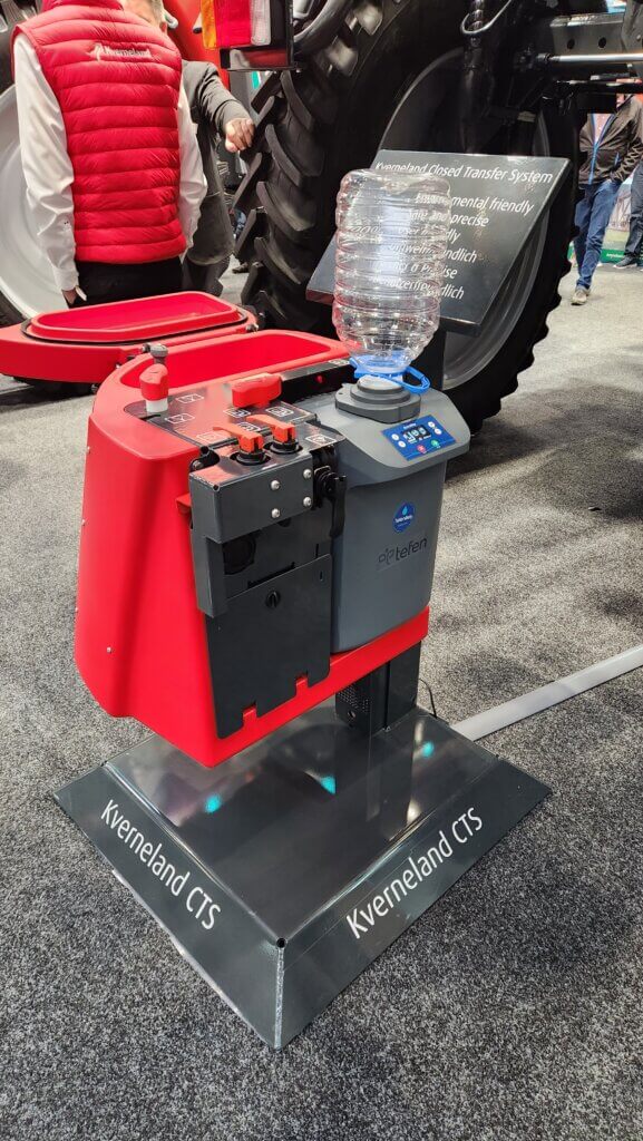
We saw one moulded into a Kverneland sprayer (now owned by Kubota) that was designed to couple with the current induction bowl. This is the first time a sprayer company has altered their design to accommodate a CTS and it points to the future.
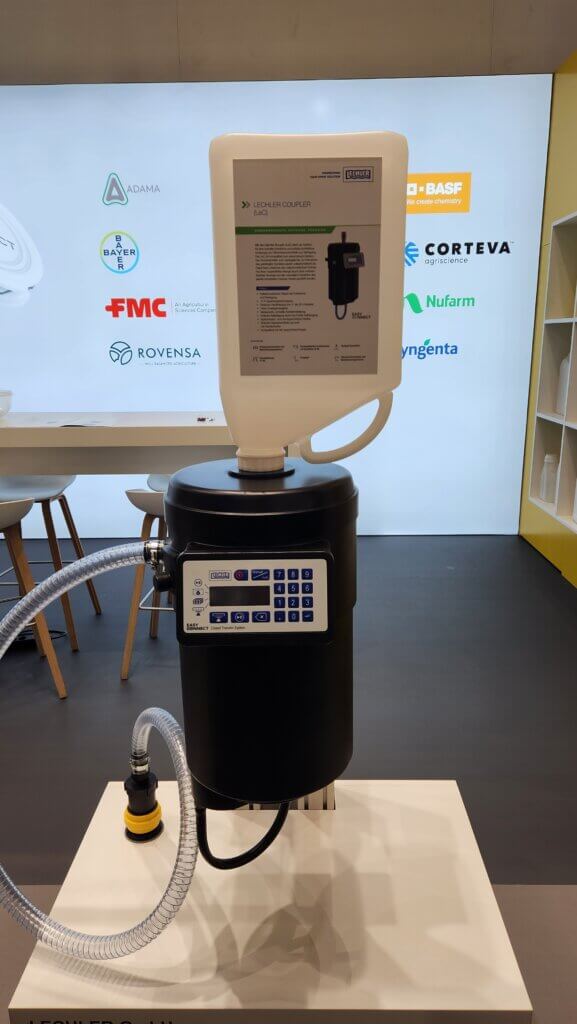
Lechler’s Coupler is compatible with the easyconnect cap and features more electrical automation in its design. It requires a 12V electric supply and creates suction (typically from the sprayer’s venturi) to draw out the chemical. A small metering motor automatically moves the probe that enters the container to adjust emptying rate. It employs a pressurized water line running at about 6 bar.
The system will be controlled via a smartphone app, where the operator can choose partial or full emptying of product containers and control the operating and rinsing processes. Rather than metering flow, the unit employs three load cells with vibration compensation to weigh product. Lechler claims this is more accurate (automatic dosing to a set volume with +/- 2.5% accuracy), because it can compensate for different product densities. The user manually enters these values from product SDS, but likely QR codes will be used in the future.
The system underwent further testing in 2024 and commercial availability is anticipated for 2025. Farmer’s Weekly covered the details of this system following Agritechnica 2023.
Aspects of Applied Biology 147, 2022 International Advances in Pesticide Application Review of ISO 21191 Closed Transfer Systems Performance Specifications. Nancy Westcott and Jan Langenakens.
This article was originally co-authored by Mick Roberts (Owner/Editor of Pro Operator Magazine) with significant contributions from Jan Langenakens (Principal at AAMS) and informed by insightful communications with both users and manufacturers of CTS. It has been updated as of January, 2025.
Tank mixing is the practice of combining multiple registered agricultural products in the sprayer tank for application in a single pass.
The Pros of Tank Mixing
Efficiency: If the timing makes sense, a single pass saves time and reduces trample/compaction. E.g. A “weed-and-feed” application of fertilizer and herbicide in corn.
Resistance management: Multiple modes of action help prevent resistance development and combat existing problems.
Improved performance: Labels may require adjuvants to condition carrier water or reduce drift (utility adjuvants) or to improve the degree of contact between droplets and the plant surface, or enhance product uptake or rainfastness (activator adjuvants).
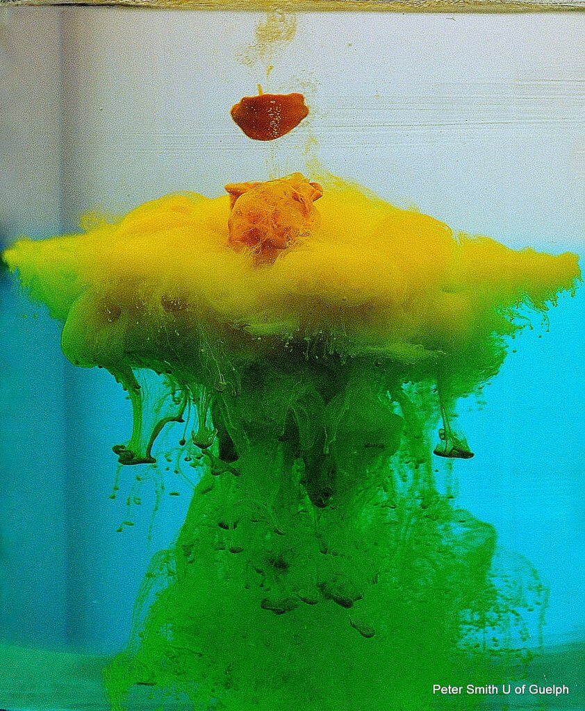
Prowl meets Roundup – A beautiful photo by Peter Smith, University of Guelph
The Cons of Tank Mixing
Tank mixing requires caution and careful investigation. Should tank mix partners prove to be incompatible, the consequences can be subtle or dramatic, but are always negative. There are two kinds of incompatibility.
1. Biological or Chemical Incompatibility
This form of incompatibility may not be immediately apparent following an application. Some level of crop damage or impaired efficacy occurs, which may impact yield or warrant an additional “clean-up” application. This is the result of product synergism or antagonism.
Synergism (Crop damage)
When products synergize, the application becomes too potent. For example, an adjuvant could affect crop retention or uptake, exposing it to more active ingredient or overwhelming crop metabolism. The result is damage to the crop we are trying to protect.
Antagonism (Reduced efficacy)
When products antagonize, the application becomes less potent. There are several examples:
pH adjusters in one product may reduce the half-life
of another product (e.g. The fungicide Captan has a half-life of 3 hours at a
pH of 7.1 and only 10 minutes at a pH of 8.2.)
Active ingredients may get tied-up on the clay-based
adjuvants in other products (e.g. glyphosate tied up by Metribuzin).
One product changes the uptake/retention of another.
For example, a contact herbicide burns weed foliage beyond its ability to take
up a lethal dose of systemic herbicide.
2. Physical Incompatibility
Physical incompatibility affects work rate and efficacy. Products form solids that interfere with, or halt, spraying. It can also make sprayer clean-up more difficult. For example, weak-acid herbicides lower the pH of the spray mix, reducing the solubility of Group 2 herbicides (i.e. imidazolinones, sulfonylureas, sulfonanilides). The oily formulation then adheres to plastic and rubber surfaces in tanks, connectors and hoses.
There are many forms of physical incompatibility:
Liquids can curdle into pastes and gels that clog plumbing to such an extent that flushing cannot clear it and a manual tear down is required.
Clogged screens
Dry formulations don’t hydrate or disperse, becoming sediment that clogs screens and nozzles. Even if they are small enough to spray, they reduce coverage uniformity. For example, a dry product added behind an oil gets coated, preventing it from hydrating.
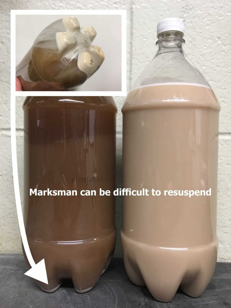
Certain product combinations may cause settling, or one partner is more prone to settling. If the sprayer sits without agitation, settled products may or may not resuspend. Even if they do resuspend in the tank, they may remain as sediment in lines.
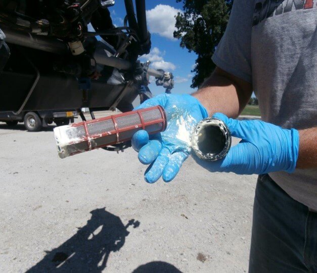
Residue in hoses – Photo courtesy of Fred Whitford, Purdue UniversityClay-based products may or may not resuspend easily in a tank. Even then, they may not resuspend in plumbing lines.
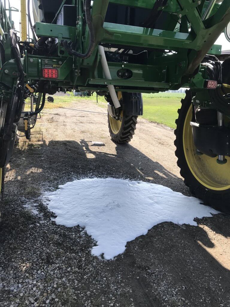
Certain product combinations may cause foaming, or one partner may be prone to foaming, causing overflows or breaking pump suction. When products foam, dry products added through the foam may swell, preventing hydration.
The Foamover Blues
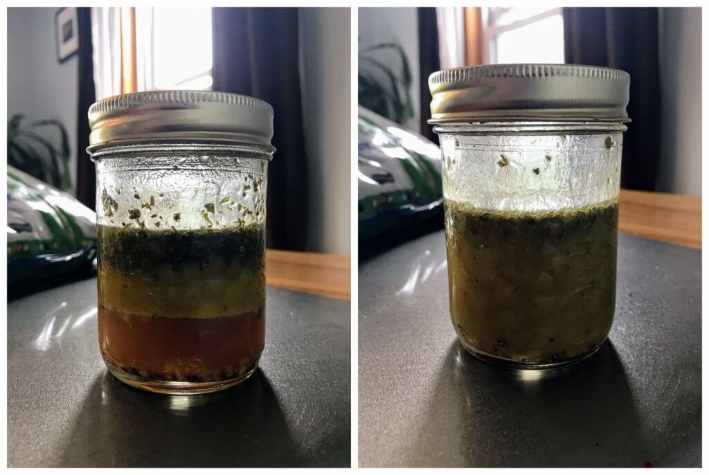
Phase separation occurs when products layer in the tank. Consider oil and water. Even with agitation, the active ingredients may not be uniformly suspended in the tank and coverage uniformity will be reduced during spraying.
Salad dressing left to rest is a great example of separation and stratification (left). Agitation helps emulsify it (right)
Due Diligence – Preventing Tank Mixing Errors
Incompatibility is often a function of the inert ingredients in pesticide formulations (e.g. thickeners, adjuvants, defoamers, stabilizers, solvents, etc.) and not the active ingredients. The more products you add to the tank, the more likely you’ll encounter an issue. It is prudent to perform a jar test to confirm physical compatibility. Remember, even if registered tank mix partners support mixing, your pace, mixing order, and water quality/temperature could cause issues.
Do not decide to try a new-to-you registered tank mix during loading. Even if you’ve used these products successfully in the past, formulations change without notice. Plan as much as possible off season when there is time to do the following:
Consult the pesticide labels
Pesticide
labels are always the first point of reference. They should be obeyed even if they
contradict conventional practices. Booklet-style labels that come with the
products are long, difficult to search and may not be up-to-date.
In Canada, it is faster and easier to go to the PMRA Label Search website and search labels in PDF format. In other countries, consult the manufacturer’s website for label information. For each tank mix partner, use <CTRL>+F to find the following keywords:
Do Not Mix
Mix
Hours
Agitation
Fertilizers
Consult manufacturer and crop advisors
You’re likely not the first to consider a certain tank mix. Learn from those that have been there already:
Consult your chemical sales representative. They
know their products best and want to see you succeed. They may have insight that
is not found on the product label.
Consult local government or academic extension
programs for an unbiased opinion.
Enlist the help of a professional crop advisor.
It is a good practice to get tank mix recommendations in writing. If something should go wrong, liability is an important concern.
If you’ve made a mess – The Reverse Jar Test
It
happens. We’ll use this real-world situation as an example:
“I mixed up a batch of MCPA 500 A and Glyphosate at ¾ recommended label rate, but then got delayed on application with a stuck drill. I came back to the sprayer and found a nasty chemical precipitate – like waxy chunks. Agitation didn’t break them down. I dumped the tank out as I didn’t want to pump it through the booms. How do I clean up the chunks in the system?”
We forwarded
this question to ag chemists Dr. Eric Spandl (Land of Lakes) and Dr. Jim Reiss
(Precision Laboratories) and developed this response:
“Wearing appropriate personal protective equipment, physically remove the “chunky” material. A lot of time can be wasted (and rinsate water created) by experimenting with various concoctions, but if you do choose to try a compatibility agent, first try it in a mason jar. If it works to dissolve the material, it can be added to the tank with water and agitated. If not, you are down to manual cleaning: hot water under pressure.”
We dubbed this process “The Reverse Jar Test”. Do not add hot water, cleaners or compatibility agents until the reverse jar test confirms success. You may create a larger problem. Of course, the best advice is to not put yourself in this position to begin with. Once again, don’t make mixing decisions at the inductor bowl – make them before ordering product.
Tank mixing regulations in Canada (January, 2025 update)
The following legislative framework is specific to Canada, so readers in other countries should consult their own regulatory authorities.
Paragraph 6(5)(b) of the Pest Control Products Act (PCPA) states that no person shall use a pest control product in a way that is inconsistent with the directions on the label. In 2020, a public consultation was held to consolidate and clarify tank mixing requirements. This led to Regulatory Proposal PRO2020-01 (Streamlined Category B Submissions and Tank Mix Labelling – July 3, 2020). Essentially, it stated that tank mixing would be allowed if there was text on the product label that specifically permitted it. This could be a specific tank mix combination, a general statement permitting mixing, or both.
A new general label statement that permits tank mixing was proposed to consolidate tank mixing information in one place on the label and allow greater flexibility in terms of tank mixing options. The prohibition against tank mixing products with the same mode of action was removed, and the reference to tank mixing with a fertilizer is now an optional component of that statement. The general label statement reads as follows:
“This product may be tank mixed with (a fertilizer, a supplement, or with) registered pest control products, whose labels also allow tank mixing, provided the entirety of both labels, including Directions For Use, Precautions, Restrictions, Environmental Precautions, and Spray Buffer Zones are followed for each product. In cases where these requirements differ between the tank mix partner labels, the most restrictive label must be followed. Do not tank mix products containing the same active ingredient unless specifically listed on this label.
In December of 2022, Health Canada released a guidance document describing the federal tank mixing policy. This document is not part of the PCPA, but is an administrative document intended to facilitate compliance by all stakeholders. Registrants have until December, 2025 to update their extension material to align with amended product labels and guidance documents. Similarly, users of pest control products will be provided the same transitional period to adjust their purchasing and production practices to align with the provisions of this document. This means the policy will be in full effect on December , 2025. After that, applicators in Canada can only apply tank mixes that appear specifically on a product label, or tank mixes of products whose labels include the new general tank mixing statement.
Summary of the guidance document
Tank mixing is not permitted when a potential tank mix partner’s label has some exclusionary statement, such as:
Forbidding mixing. E.g. “Do not mix or apply this product with any other additive, pesticide or fertilizer except as specifically recommended on this label.”
Limiting tank mixes to only those specifically listed on the product label.
During the label transition, guidance relating to tank mixing may be found under a section specific to tank mixing, and/or under other sections as in the following examples:
Directions for use: E.g. “When tank-mixes are permitted, read and observe all label directions, including rates and restrictions for each product used in the tank-mix. Follow the more stringent label precautionary measures for mixing, loading and applying stated on both product labels.”
Buffer Zones: E.g. “When tank mixes are permitted, consult the labels of the tank-mix partners and observe the largest (most restrictive) spray buffer zone of the products involved in the tank mixture and apply using the coarsest spray (ASABE) category indicated on the labels for those tank mix partners.”
Resistance Management: E.g. “Use tank mixtures with [fungicide/bactericides/insecticides/acaricides] from a different group that is effective on the target [pathogen/pest] when such use is permitted.”
If there are no directions on the labels, don’t tank mix them.
If your situation does not fit these examples, the following table (Appendix A at the bottom of the Guidance Document), lists several other examples examples of different tank mix wording scenarios for registered pest control products.
Table 1: Permissibility of tank mixing based on various combinations of label statements related to tank mixing
Product X label says
Product Y label says
Can I tank mix? (Y/N)
Nothing (silent on tank mixing)
Nothing (silent on tank mixing)
N
General tank mix statement
Nothing (silent on tank mixing)
N
Nothing (silent on tank mixing)
General tank mix statement
N
General tank mix statement
General tank mix statement
Y
General tank mix statement
Tank mix with Product X
Y
Tank mix with Product Y
General tank mix statement
Y
Tank mix with Product Y
Nothing (silent on tank mixing)
Y
Nothing (silent on tank mixing)
Tank mix with Product X
Y
Tank mix with Product Y
Tank mix with Product X
Y
Tank mix with Product Y
Exclusionary statement (and label does not include a specific Product X tank mix)
N*
Exclusionary statement (and label does not include a specific Product Y tank mix)
Tank mix with Product X
N*
*There may be registered labels that have tank mix scenarios like this. Note that this is not allowed for new tank mix label amendments. Further, any product labels that have tank mix scenarios like this must be amended to alleviate the contradictory scenario. To do this, using the last scenario in Table 1 as an example, one of the following must occur: 1) remove the Product X tank mix from the Product Y label, 2) remove the exclusionary statement from the Product X label, or 3) add a specific tank mix for Product Y on the Product X label. Source: PMRA Guidance Document Tank Mix Labelling 2023
Tank mixing adjuvants
According to the PMRA, the rules surrounding the tank mixing of adjuvants remain the same as they have been since 2009, and are not included under the new guidance document. While the PCPA does not reference adjuvants specifically, they are prescribed to be pest control products in the regulations (Pest Control Products Regulations s.2(b)). The general reference in the PCPA that applies is s.6(5)(b).
Therefore, in the case of activator adjuvants, the label for at least one tank mix partner must specify the use of an adjuvant, and only registered adjuvants labeled for the crop and for tank mixing are permitted. For example, tank mixing the herbicide Reflex with a registered soybean oil adjuvant not labelled for the use, or with an unregistered food grade activator adjuvant, would not be acceptable. Utility adjuvants have registration numbers, but their use is not prescribed or specified on pesticide labels, leaving their use to the discretion of the operator.
For more information on Canada’s Tank Mixing Policy
In late 2022, Australia’s GRDC released a comprehensive guide on pesticide mixing and batching (within the context of the Australian agronomic environment, of course), which can be downloaded for free, here.
Finally, you can watch a 2021 presentation on tank mixing (below). It was delivered to a grape growing audience, but much of the content applies across agriculture. There are a few “oops” moments where I didn’t say quite what I meant. I misread the Sencor dissolution / filtration work. And, I really didn’t answer the last question about mixing herbicides. The answer should have been to consult labels and local resources, such as OMAFRA’s Crop Protection Hub. Note that any discussion of Canadian regulatory policy may have changed in light of the new 2022 Guidance Document.
This article was co-written with Mike Cowbrough, OMAFRA Weed Management Specialist – Field Crops
In 2019 we evaluated the spray coverage from nine application methods on corn silks. The results showed that a directed application from drop hoses (aka drop pipes, drop legs) suspended in between the rows gave significantly higher deposits. The results led us to wonder if the superior coverage from a directed application translated to improved yield.
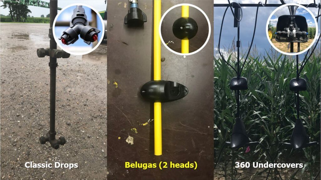
Around this time we started considering the Beluga Drop Hose developed by Agrotop (Germany) and distributed by Greenleaf Technologies (USA). Originally designed to apply neonicotinoids in canola, we found that the stiff-but-flexible hose did not tend to deflect or sway during an application. Further, their unique low-profile nozzle body had less potential to cause mechanical damage or otherwise snag in dense canopies. Unlike homemade drop pipes or other commercial solutions such as the Y-Drop with 360 Undercover, the Belugas were lightweight, simple to install/remove, and did not need a break-away section to prevent damage.
Three examples of directed application systems. Left: Homemade drop pipes and a TeeJet QJ90-2-NYR split nozzle body (inset). Centre: Beluga drop hose with streamlined nozzle body (inset). Right: Y-Drop side-dress drop pipes with Yield 360 Undercover option (inset).
In 2021 we initiated a four-year trial with the Beluga drop hose system in Port Rowan, Ontario. Our objective was to evaluate return-on-investment based on yield using two pesticide regimes. Treatments were established for conventional overhead technology, directed applications (i.e. the Beluga) and unsprayed checks.
Construction and Installation
We ordered 150 cm (60″) drop hoses with two nozzle bodies each so we could customize them. The instructions were in German, but after running them through translation software we were confident in how to proceed (download the translated copy here). We started by determining the hose length.
Hose Length and Boom Spacing
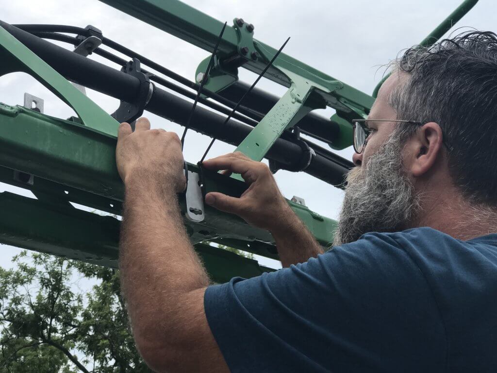
We started by temporarily fixing the mounting plates to the boom using quick ties because we wanted to ensure they did not interfere with boom folding. The drop hose quickly and easily “keys” into the plate allowing it to swing freely and find plumb. The corn was planted on 76 cm (30″) spacing so we aligned the plates with the alleys to permit the drop hoses to move between the planted rows. Each hose is plumbed to the nearest nozzle body via a quarter-turn quick-connect coupler.
Temporarily attaching mounting plates every 30 inches to correspond with corn alleys. The Beluga keys into the mounting plate and is then plumbed into the sprayer via a quarter-turn quick-connect coupler that attaches to the nearest nozzle body.
The drop hose had to clear the ground but still be long enough permit nozzle bodies to span the target region in the canopy. We later learned to cut the excess hose closer to the lowest nozzle body. This eliminated a source of pesticide collection (like a boom end) and prevented them touching the ground and “walking” as occasional contact would cause them them to flex and leap forward.
Target Zone and Nozzle Body Spacing
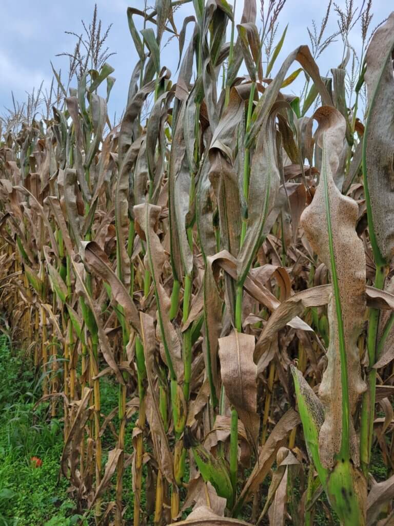
Before we could permanently install the nozzle bodies on the drop hoses, we had to decide what our target was. This required us to establish a primary coverage zone within the corn. Dr. David Hooker (University of Guelph) experimented with directed sprays (triazoles) and leaf disease control in the 2010’s. Dr. Hooker noted that leaf diseases were controlled above the ear to the flag leaf, and postulated it may be due to xylem mobility (i.e. acropetal movement) of the fungicides used at the time. This concept warrants further investigation with modern fungicides, especially with the need to control tarspot and reduce DON risk in SW Ontario.
Tarspot in corn – Southwest Ontario, 2023
Given that the nozzles would be about 38 cm (15″) from the stalk, we elected to use 110° flat fan nozzles on two nozzle bodies spaced 50 cm (20″) apart to increase the swath. Our objective was to protect against foliar disease, so the bottom nozzle was aimed approximately at the ear (for silk coverage) and the upper nozzle covered the higher foliage without being so high as to spray out of the canopy. Between gravity, the wake of the drop hose, and the initial angle of the spray, all surfaces received some degree of spray coverage no matter their orientation or depth. This was later confirmed using fluorescent dye.
It has been suggested that this target zone may not be ideal for all hybrids, and that an overhead component should be included. However, we felt this was the most efficient distribution of the spray given Dr. Hooker’s observations and the results from the 2019 spray coverage work referenced earlier.
Each drop hose was suspended on 76 cm (30″) spacing to correspond with the centre of each alley. Nozzle bodies were spaced 50 cm (20″) apart to cover the primary target zone within the canopy. The outer two drop hoses only had inward-facing nozzles to contain the treatment. We later cut the excess hose closer to the lowest nozzle body.
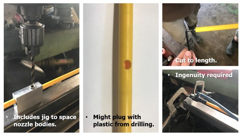
Using the jig provided, we drilled holes for the two nozzle bodies. Then we blew-out the hoses to clear them of any plastic shavings that could plug nozzles. The hoses were cut to length and the end plug was installed with a hex key. Once we found a rhythm, the assembly went quickly and easily. Expect assembly and mounting to take a day.
Customizing the hose length and nozzle spacing. We built our own clamping jig to hold the pipes steady.
Plot Design, Sprayer Set-up and Chemistry
The study took place on 11.3 ha (28 acres) spanning two fields. The corn variety was Pioneer P0720AM, which has a Gibberella Ear Rot rating of 4. Four overhead treatments, four directed treatments and four unsprayed checks were arranged in a random block design for each of two fungicide regimes (n=8 for each treatment per year). Each treatment area was between 1.05 and 1.10 acres..
The sprayer was a self-propelled John Deere R4038 with a rear-mounted 36.5 meter (120′) boom. Treatments were eight corn rows wide, so the boom was nozzled to permit all three treatments in a single pass. Travel speed was between 8.85 – 11.25 km/h (5.5 – 7 mph) and the application volume was 225 L/ha (20 gpa).
Nozzle choice is indicated in the following table. Note that after the first year, we elected to use a smaller droplet size on the Belugas; This gave the advantage of higher deposit density with little or no risk of drift from inside the canopy.
Year
Broadcast (Overhead)
Directed (Beluga)
Unsprayed Check
1
TeeJet AIC11005’s on 15″ centres
4 Airmix 110015’s per drop on 30″ centres
Nozzles blocked
2,3,4
TeeJet AIC11005’s on 15″ centres
4 Spray Max 110015’s per drop on 30″ centres
Nozzles blocked
Treatment nozzles by year
Two tank mix regimes were applied each year, as indicated in the following table. Tank Mix 1 was used each year. Tank mix 2 changed based on pesticide availability and the farmer cooperator’s preference. The insecticide “Delegate” (50 g/ac) was also included in each tank mix. However, there was very little evidence of the target pest (Western Bean Cutworm), so the impact of Delegate will not be discussed. Further, to keeps matters simple, we will not be discussing the relative efficacy of each tank mix in this article. Instead, the results are combined and only the application method and total cost of fungicides will be compared in this study.
Tank Mix (Year)
Product
Rate (/ac )
Tank Mix 1 (all)
Miravis Neo
405 ml
Tank Mix 2 (2021)
Headline AMP + Caramba
303 ml + 405 ml
Tank Mix 2 (2022)
Veltyma + Proline
202 ml + 170 ml
Tank Mix 2 (2023)
Veltyma DLX
202 ml + 405 ml
Tank Mix 2 (2024)
Veltyma DLX
202 ml + 405 ml
Tank mix treatment rates by year.
Qualitative Results
Leaves
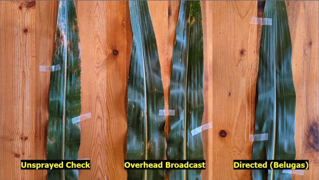
In all four years, a qualitative comparison of randomly-selected ear leaves showed less evidence of disease in the fungicide treatments compared with the unsprayed check. Generally, there was also less evidence of disease in the Directed application treatments versus the Overhead broadcast application treatments.
A typical random sampling of ear leaves were selected from multiple locations in the treatments. Leaves appeared cleaner in the fungicide treatments versus the unsprayed checks. Leaves from the Directed applications seemed cleaner than the Overhead broadcast applications.
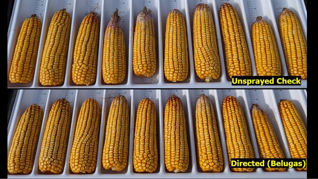
Cob Size / Quality
In all four years, preliminary samples showed evidence of disease and tapered-ends in both fungicide treatments and the unsprayed checks, but trends indicated improved size and quality of the cobs from fungicide treatments. It was difficult to discern any difference between Overhead and Directed application at this stage.
Typically, preliminary sampling showed less incidence of disease in the fungicide treatments but no obvious difference between methods of application.
Quantitative Results
Net Revenue
Each treatment yielded corn with different moisture levels, so we chose not to compare bushels per acre harvested. Instead, we calculated net revenue for each year based on the current market values in the Port Rowan area. We normalized the treatment yields by moisture level and calculated their relative drying costs. Then we accounted for the other inputs (see list below) using the following formula:
Net Revenue (CDN) = Seed Yield × Corn Sale Price – Drying Cost – Treatment Cost
Item
2021 ($)
2022 ($)
2023 ($)
2024 ($)
Corn Sale Price (/bu)
6.00
8.00
6.50
6.00
Custom Spray Cost (/ac)
12.00
12.00
15.00
15.00
Drying Cost based on Moisture Levels (/bu)
0.58-0.64
0.60-0.69
0.49-0.56
0.47-0.54
Tank Mix 1 (/ac)
16.66
18.24
18.50
18.86
Tank Mix 2 (/ac)
15.75
28.52
22.09
22.49
Net revenue input costs and prices by year in Port Rowan, Ontario
Averages were calculated for the eight replications for each treatment. These average yields (bu/ac), moistures and ROIs ($/ac) are presented for each treatment, for each year, in the table below. The average values of all four years are also presented in this table. With few exceptions, it always paid to spray, and the directed application produced a higher yield than the conventional overhead treatment.
Year
Treatment
Yield (bu/ac)
Moisture (%)
AverageROI ($/ac)
1
Broadcast vs. Check
-2.26
+0.58
-0.49
1
Directed vs. Check
+3.48
+0.60
+20.93
1
Directed vs. Broadcast
+5.74
+0.01
+21.42
2
Broadcast vs. Check
+9.79
+0.22
+52.48
2
Directed vs. Check
+14.56
-0.04
+89.14
2
Directed vs. Broadcast
+4.77
-0.26
+36.66
3
Broadcast vs. Check
+8.40
-0.20
+23.70
3
Directed vs. Check
+22.7
+0.20
+117.10
3
Directed vs. Broadcast
+14.4
+0.40
+93.40
4
Broadcast vs. Check
+45.7
+1.00
+244.37
4
Directed vs. Check
+43.7
+0.80
+232.09
4
Directed vs. Broadcast
-2.10
-0.20
-12.28
All
Broadcast vs. Check
+13.40
+0.40
+69.07
All
Directed vs. Check
+19.60
+0.40
+107.00
All
Directed vs. Broadcast
+6.20
0.00
+37.93
Final accounting. Bold indicates a desirable outcome, while italics signify an undesirable outcome (n=8 per year).
Return on Investment
Given that costs changed each year, it’s not ideal to average the final costs. However, doing so gives a relative indication of the value of spraying versus spraying with overhead systems versus spraying with directed systems.
Directed (Belugas) vs. Unsprayed check: Profit of $107.00/ac CAD
Directed (Belugas) vs. Broadcast (Overhead): Profit of $37.93/ac CAD
Broadcast (Overhead) vs. Unsprayed check: Profit of $69.07/ac CAD
Perhaps a more realistic review of the ROI is to calculate how many acres were required to pay for the Beluga system each year. In other words, how many acres would a grower have to spray for the profit to offset the cost of purchase? This value was different each year due to changes in costs and relative disease pressure.
In 2021, 48 Belugas on (30″ centres) and 192 110 degree flat fans was $8,400.00 CDN. 2022: $8,600.00. 2023: $8,800.00. 2024: $8,890.00. Perhaps it was demand, or a change in dealers, or perhaps it was tariffs (or both) but in 2025: $13,500.00. Note that the break even point spanned from roughly 40 to 400 acres, but on average was less than 100 acres.
Corn acres required to offset start up costs of the Beluga system from 2021-2024. A broad description of growing conditions and disease pressure in the test fields is noted for context. n=8 each year.
While now a little out of date, the following video filmed by Real Agriculture discusses the return on investment based on 2021 and 2022 data.
Mycotoxin Assays
We submitted samples for lab analysis of mycotoxins for each treatment, annually. However there are many factors that influence ear mould pathogens, and we did not see any clear correlations between the fungicide, application method, or even the unsprayed check with the level of Deoxynivalenol (DON aka vomitoxin) or zearalenone detected.
The Drop Hose Experience
While cost and efficacy are key considerations, we felt it was also important to describe the utility and user-experience. This study focusses on the Port Rowan trials, but over the years several other Ontario farmers have adopted the Beluga system and reported on their experience. We have included their observations:
Installing and uninstalling the drops took roughly 90 seconds apiece, including moving the ladder.
Deflection was minimal, even when they were dragged perpendicular to the rows through headlands.
The factory mounting bracket permits the drop to be “keyed in” from either side, however this may have led to drop hoses occasionally detaching in shorter corn stands and on sharp turns. The weak point may be the plastic hose barb, which can be damaged if the drops detach from the mounting plates. Rather than the current slot positions of “9:30 and 2:30”, “11:00 and 1:00” may prevent detachment. One dealer, however, has redesigned the mounting plate and linkage to compensate.
Initially, it was a little unnerving not being able to see the spray but the operator quickly got used to it (see video below).
There was no issue folding the boom or driving between fields with the drops installed. They did note that the lugs on the front tires did contact the drops on tight turns, but adjustments were made.
There were issues with other sprayer types (e.g. New Holland Guardian) when folding the booms. Drops did not hang plumb during transport. One dealer developed new linkages to account for differences in boom design.
The drop hoses rinsed as easily as any nozzle. One dealer developed new hose-end plugs to facilitate rinsing.
There were initial concerns that using 015’s nozzles to maintain the target 20 gpa might cause plugging issues, but none occurred.
The drops were resilient. The operator bent the hoses by lowering the boom and then dragged them along the ground. They returned to plumb and appeared undamaged. One operator elected to use a NutraBoss Y-Drop mount to stiffen the top few inches of the Belugas (image below) but no other user found this necessary.
Once removed, the drops stored compactly and easily on a utility shelf, repacked in their original box or hung on the shed wall.
Beluga drop hoses mounted on a NutraBoss frame
Custom Operators
Some custom operators have also begun to use the Beluga system and have reviewed it positively, but others question the fit. The latter feel this technology makes more sense for a home farm operation where the drops can be cut to a size that aligns the nozzles for a specific combination of boom height and corn variety. The concern is that a custom operator would have to adjust boom height (if not already maxed) or swap drop hoses to configurations that align correctly with the client’s crop. However, four years in, early adopters have collectively sprayed more than 20 different corn varieties with multiple sprayers and have had no issues reaching the target zone.
Additionally, our study has focused on 20 gpa where some custom operators would prefer 15 gpa. Reducing volume necessitates a change in travel speed (may not be practical) or a reduction in operating pressure (may increase average droplet size). It would be inadvisable to drop from 015’s to 01’s (think plugs and misty spray).
Both limitations translate to additional cost (currently about $2.00 CDN per acre) to a client. The value proposition becomes the added cost for an efficacious application versus the potential losses should conventional application methods fail to control devastating diseases such as Tar Spot and Northern Corn Leaf Blight.
Adoption in North America
Beluga drop hoses are distributed by Greenleaf Technologies in Covington, Louisiana and resold through dealers in the USA and in Ontario. It is not possible to determine how many sets have been sold, but if a boom is 100′ to 120′ and drops are placed every 30”, then a set would be 40-48 hoses. We started reporting on their value in corn protection in 2021. The following sales figures are annual sales (i.e. not cumulative) from Greenleaf Tech. This includes the 36″ hoses, which may or may not be used in corn. These figures will be updated annually:
Conclusion
With the exception of 2024, which was essentially parity between Overhead and Directed methods, we saw an annual increase in mean net revenue from corn sprayed using a directed application. The low price point, ease of use, and high rate of return make this an attractive proposition in corn production.
Thanks to Petker Farm Ltd. and other early adopters for participating in the study. Thanks to Corteva and Syngenta for contributing the pesticides used.