When operators winterize their sprayers, they should remove all the tips and store them separately. Many store them in large pails with lids. Calibrating the sprayer just prior to winterizing will indicate if the nozzles should be stored, or replaced. Let’s assume each tip flow rate is within 5% of the average output and no more than 5% more than the manufacturer’s pressure tables. Yes, industry standard is 10%, but I always wonder how the spray quality suffers with that much wear. Nozzles are, comparatively, a cheap replacement and it’s not worth skimping. Learn more how to check nozzle flow rate, here.
Just like any other part of the sprayer that comes in contact with spray liquid, nozzles (and strainers) should be cleaned regularly. And, just like any other part of the plumbing, the best way to do that is to dilute any residues via a series of rinses. For a more rigorous cleaning, one of the intermediate rinses should include a detergent, and soaking during this step is an excellent practice.
The orifice of any nozzle is delicate, either machined or molded to exacting standards. Even small changes to the orifice shape results in distorted spray (e.g. spray comes out at undesirable angles), a change to the rate (typically more volume per minute) and a change in the spray quality (typically larger median droplet size). If foreign objects or residues remain in the tips, the subsequent spray job may be less accurate and even damage the tips.
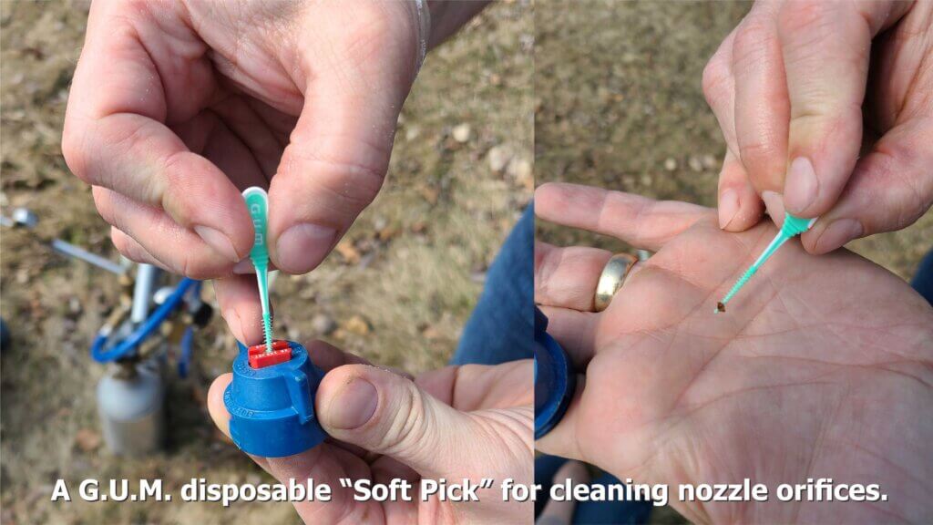
In the case of air induction nozzles, which are essentially the standard on most boom sprayers, debris and weed seeds can plug the air-intake ports. When that happens, the nozzle will not function as intended. So, while the occasional soaking of nozzles does a great deal of good, they may also have to be scrubbed. Don’t use picks or reamers! There are nozzle cleaning tools out there, but they’re basically toothbrushes so save your old ones (and mark them clearly). Soft bristles are the way to go for removing stubborn residues and cleaning any tip orifices, but we found a nifty new way:
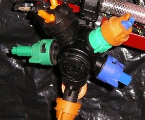
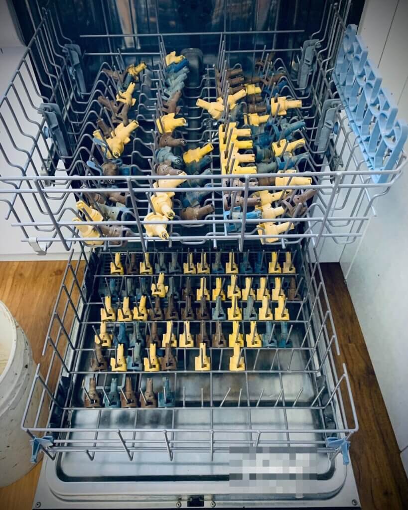
Occasionally we receive photos like the one below and we’re asked what we think. Well, just the same way we don’t recommend cleaning your sprayer overalls in the family clothes washer, we also don’t recommend the use of dishwashers for nozzles.
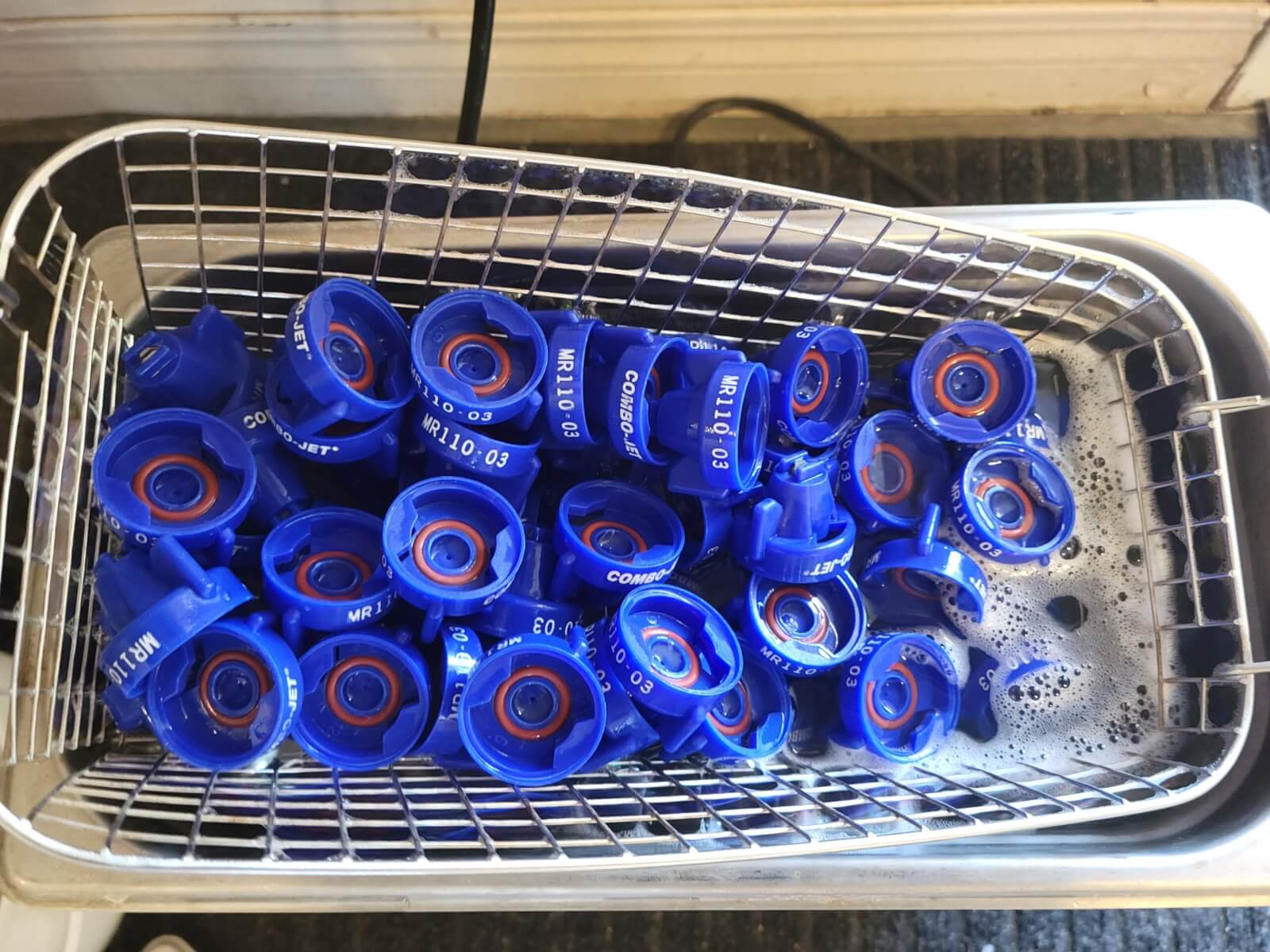
In an interesting experiment, Lucas Olenick of Wilger tried cleaning tips in a heated ultrasonic cleaner. We haven’t tested this and we don’t know what heat and vibration might do to poly and ceramic components, but surely it’s no more aggressive than hot, soapy water and a bristle brush. Lucas tried several durations with and without detergent and arrived at this recipe:
“For tough, non-water-soluble pesticides, around 8+ hours in a heated ultra-sonic cleaner with (Dawn) dish soap to come out like brand new. Other solvents may speed this up, but I’d generally suggest against heating solvents at any concentration. For water-soluble pesticides, expect to be within the 3-6+ hours for the first time to be confident enough in not having to flow-test each of the nozzles. With any pesticides, ensure proper care in handling contaminated nozzles and rinsate after cleaning nozzles.”
Don’t have a heated sonic cleaner? No problem. Here’s a step by step:
- Wearing gloves, remove all nozzles, strainers, rubber gaskets and tips from the sprayer.
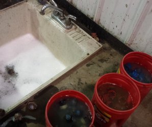
- Put them in a large plastic pail and cover them in warm water. Leave them to soak.
- Drain the pail, but be aware that the rinsate will have pesticide residue.
- Fill a second pail with a solution of the same commercial detergent used to clean the sprayer.
- With a toothbrush, scrub the caps, gaskets, strainers and nozzles to remove any residue. Some nozzles can be pulled apart to expose the mixing chamber and facilitate cleaning.
- Once scrubbed, leave all the parts to soak in the detergent solution.
- Drain the solution, which will contain trace amounts of pesticide, rinse the parts with water and reassemble the nozzles.
While you’re at it, drop those filters and scrub them alongside the tips. This may seem extreme, but of all the technology on a sprayer, the nozzle has the biggest impact on the effectiveness and efficiency of the spray job. Take the opportunity over the winter months to clean and inspect the tips for damage so the sprayer is ready for calibration in the spring.
Thanks to Jason Boersma (@RVFBoys), Ridge Valley Farms, Ontario, who sparked this article with his tweet: “Great job for a cold winter day, soak & clean all your tips to be ready for spring also saves on down time!”