There are many factors that affect the work rate of an airblast application. If an operator can improve their work rate, without compromising spray efficacy or safety, they improve operational efficiency and save money.
But how does each variable factor in? Is it worth the cost of a tender truck and operator to fill more efficiently? Should you upgrade to a multi-row sprayer? Should your next planting have longer rows? We have a simple calculator that can help you make these decisions. You can build and compare multiple scenarios to explore the relative impact of small changes to your typical spray program. We recommend making only one change for each scenario so you can better understand the results. Print the comparison page for your records.
Whether you’re a sprayer operator, or a manager of sprayer operators, this exercise will help you see your spray program in a whole new light. Download a copy of the Airblast Budget and Work Rate Calculator and explore your productivity. You must have Excel to run the spreadsheet, and you must permit the use of macros (you’ll be prompted to accept).
Spoiler: It’s amazing how changes to travel speed have only a marginal impact on work rate. Often less than 60% of the total spray job is spent actually spraying!
If you’d like to see just how productive you can be, check out this rare (possibly unique) sprayer from Ed Oxley Farms in Michigan. Built on an OXBO 7550, this sprayer is the fourth iteration of a concept developed over the last 20 years by Ed Oxley Farms and ag engineers from Michigan State University.
Capable of spraying five rows at a time, this self-propelled beast is a hybrid wrap-around and targeting-tower system that uses CurTec spray heads equipped with tangential fans and wire-mesh basket rotary atomizers.
That’s not dribbling – that’s purging the boom prior to spraying.
It sprays a mere 150 L/ha (~ 15 gallons/acre) at a ripping 13 km/h (~8 mph), as seen on the Ag Leader monitor below.
When row spacing and turn time are accounted for, that means it’s capable of covering almost 15 hectares (~40 acres) per hour.
And, when not spraying grapes, the boom can be swapped to make it a high-clearance corn sprayer. It doesn’t get much more efficient than this.
The following videos will show the view from inside and outside the cab. Note that the row that’s straddled is sprayed from an overhead spray head mounted to the centre rack behind the sprayer. The two adjacent rows are covered from one side from vertical spray heads mounted on the chassis. Finally, the boom holds two more overhead spray heads for the outer-most rows.
Ideally, the boom-mounted spray heads would be suspended vertically inside the row, but it makes for such a wide turn radius that it would take too long to turn… assuming there was enough headland to allow it. They’re also swept-back to minimize the turn radius and reduce the amount of airborne spray that deposits on the sprayer itself.
A clever design that makes a few compromises to ideal coverage in order to improve productivity. The balance works for them and this sprayer might be a sign of things to come in horticultural crop production systems. Want to see how your sprayer stacks up? Download the calculator and see where you might be able to make improvements.
I was excited. Today would be my first in a series of drive-along experiences with Ontario sprayer operators. However, to get from my home in Southwestern Ontario to Newmarket, I would have to cross Toronto. This is not my favourite thing to do. But, Dean Solway, Plant Healthcare Supervisor with Shady Lane Expert Tree Care, was based out of Mount Albert and he liked to start at 6:00 am. So, a hot shower and a hot coffee (not necessarily in that order) gave me the emotional support I needed to throw elbows on the parking lot we call the 401.
It was strangely unsettling to see Tim Horton’s closed, and equally odd to see only a handful of cars on the highways. That may have been the fastest, smoothest drive through Toronto that I’ve ever had.
5:45
I arrived at the 10-acre lot that has been owned by the company for the last 45 years. I walked past a small, 500 tree nursery they’d recently planted to find Dean in the office. He was busy checking bookings for the day and assigning jobs to his three Plant Health Care trucks (PHC1, 2 and 3). More on those later. After a few introductions, I faded into the background and let them get on with things.
Dean was ensuring the routes made sense and that everyone was ready to go. He explained that the week’s bookings were set each Friday, but that things could always change at the last minute. Front-line administration would handle client calls and communicate with the trucks throughout the day. They also ensured the clients were given at least a day’s notice that someone would be coming to treat their plants. Interestingly, the company is also required to inform the client’s neighbours. Dean said it helped avoid potential conflicts such cars, sunbathers or laundry left in the path of potential overspray. Not that such things ever happen, of course.
Operators kept referring to “The Board” which showed their daily assignments. With 2,800 clients scatted over Brechin, Barrie, Oakville, Pickering, Oshawa and downtown Toronto, thoughtful planning and clear communication were critical requirements.
I eavesdropped as Dean talked to a new hire about safety. Filter checks/replacements, face shields, gloves and orange vests were assigned, and I’m confident that it wasn’t staged for my benefit. Operator safety was a theme that came up throughout the day and it was clear Dean took it seriously. As the trucks got ready to roll, he fielded random questions about pesticide rates, tank mixes, crop staging and general agronomy as he double-checked that each truck was properly loaded.
I learned that standard operating practice was to regularly test the equipment and plumbing in each truck. Experience showed it was easier and less contentious to deal with minor leaks and similar issues in the yard than on a Toronto highway or even worse, at a client’s home. That took us outside.
6:15
Each truck was equipped with a tablet containing SDSs for all the products they use, PDFs of the pesticide labels and a hyperlink to Health Canada’s Pesticide Label Search website. Many of the products used by arborists are biorational / organic, either by choice or because labels do not permit the use of many conventional pesticides in urban environments. I felt a bit of team-pride when I was told that OMAFRA’s Pub 840 is a significant reference document for the company.
As he checked the trucks, Dean noted that it was important to explain to clients that eradicating pests isn’t always possible. Most often it’s about maintenance. For example, today would predominantly be about fungicide applications. Ornamental fruit trees such as crab apple were at risk of scab infection and the window for protection was narrow. Far be it for me to bring up climate change, but Dean did mention that this was the earliest he’d had to apply these products in nine years.
Protectant fungicide treatments need time to dry to be effective. If it were to start raining steadily inside two hours following the application, Dean said the client would be eligible for a re-application ASAP. According to OMAFRA Publication 840, four applications were permitted for this chemistry, and clients were scheduled to receive three at regular intervals over four weeks. That gave time for the applicator to rotate back around, and it left capacity for a possible re-application if required.
Incidentally, I am a master of foreshadowing.
The Trucks
PHC1 and PHC2 were designed to apply plant protection products. PHC3 was strictly for fertilizer and carried an extra 450 L just in case it was needed throughout the day. To remain flexible and efficient, the fertilizer applicators had to be able to take advantage of opportunities if the schedule changed. Returning to reload would be a big loss of productivity, so a little extra onboard was reasonable insurance.
Dean explained that all the trucks were filled either the morning of, or the night before, depending on the product. In the case of compost tea, it’s a three-day process that requires a lot of planning. It must be applied at less than 50 psi to prevent mechanical damage to the living component of the mix. It can be applied to the soil or as a foliar treatment.
We’d be riding in PHC1, which had a single tank subdivided into four separate 170-gallon tanks. The reel was a 60 amp electric auto reel with 300 feet of high-pressure hose. The pump was an AR 813 diaphragm pump, and the motor was a 20 hp twin cycle Vanguard and capable of producing up to 300 psi which is sometimes needed to reach the tops of the highest trees. Dean helped design this system himself and grinned when he said that even as low as 150 psi, you can feel the pistol “kick” in your hand.
Speaking of which, the hose terminated in a quick-connect that allows the operator to swap between a pistol for nearby targets, and a long-barreled rifle for more distant targets. There was also a manually pressurized two gallon bottle sprayer for when the hose-and-gun assembly simply wouldn’t reach.
The last thing Dean checked was that each truck had cleanup equipment, including detergents for any overspray accidents. He explained that most clients want no sign of the trucks coming, going, or having ever been there. That might mean washing away speckles on cars and windows, or marks from the hose being dragged on stonework or past beds and gardens. I’ll share my observations on how urban spraying seems to be viewed by the general public later on.
6:45
We’re on the road, passing through Newmarket in the York Region before slipping into stop-and-go traffic on the 404. We aren’t five minutes out before Dean’s phone rings. PHC1 is essentially his office, and he remains in communication via a work phone and headset, relying on a dedicated GPS to guide him from client to client… when the maps are accurate, anyway.
As we drive, Dean notes that rain is forecast so we’ll do as much as we can. He’s set up a linear route going to the furthest client first and working our way back. That way, if it does rain, it will be easier to reschedule because the clients are closer to the yard. He also designs routes that keep the trucks in single neighbourhoods. It’s more efficient and jumping on and off the 407 is an expensive proposition, so they use it judiciously.
7:40
According to the docket, we were slated to spray two 12-foot Siberian Crab-apples in the client’s back yard. We pulled up and hopped out. Dean walked us to the back of the house saying, “Let’s go find our patients”. I liked that.
The Process
Once located, he assessed the trees’ health to ensure the application was appropriate, and then scanned the area. He explained that an arborist had to be very mindful of the surroundings. He ensured nothing was in the path of the hose or the spray, established wind direction, and then (based on tree height and our distance from the truck) estimated the pressure we’d need for the pistol attachment to reach to the treetops.
We returned to the truck and Dean opened the side to put on his PPE. At the same time, he gave me a short safety lecture. Basically, if I saw anything leaking (on or under the truck) I was to turn off the engine immediately and we wouldn’t go anywhere until we figured out and remedied the issue. Also, should something happen to Dean, I was to call 911. Rest assured, there were no such issues that day.
He ensured the pressure regulator was completely backed off, opened the intake and return valves on the fungicide tank, attached the pistol to the hose and started up the motor. Then he adjusted the regulator to get us to 150 psi. It was obvious he’d performed this dance many times and as he went through the motions, he noted that it was important to get comfortable with the equipment but to always be respectful of it. Then he partially-closed the side panel to reduce the motor noise and started dragging out enough hose to reach his patients.
Standing upwind some distance away, I watched Dean work that first tree. He started with a few, short “test shots” into the ground to get the product to the pistol, and to adjust the width of the spray cone. Then a couple more test shots to the top of the tree to gauge the wind and the pressure. I watched him adjust the nozzle to a tighter stream and start circling the tree, spraying in short bursts until he was satisfied he’d achieved the coverage he was looking for.
Then he detached and drained the pistol before starting back to the truck. I asked what kind of coverage he was looking for and he said the standard was 90% of the canopy covered by at least 90%. That was startling to me given that our unofficial goal for most dilute applications in perennial tender fruit, pome, cane and berry is 100% of the canopy covered, but to a minimum threshold of ~15%. It’s likely due to the different chemistries (I noted earlier that urban applications tend towards biorational products). And, practically speaking, airblast sprayer operators cannot slowly circle a tree, aiming at trouble spots with an endless volume of water. Despite these differences, both methodologies seem to produce acceptable results.
The Label Dilemma
I’ve always been sympathetic of sprayer operators working in three-dimensional crops. Interpreting a North American label’s frustrating lack of guidance when it comes to water volumes for non-arable crops places a lot on the operator’s shoulders. I’ve discussed this disconnect (and proposed solutions) in several other articles. I’ve even co-written a book about it. The problem was particularly acute, here.
Ideally, one would evaluate the target tree’s planted area (which may or may not include an associated portion of alley) and work out the amount of formulated product required for that area. Then, that product must be dissolved or suspended in carrier (typically water) and that gives us the spray mix. Finally, working from the rate the sprayer emits, the operator would determine how much time would be needed to cover the target tree without over- or under-dosing. A good example of the process is found here.
But… how much water is the right amount? How do we reconcile having to achieve such a high degree of coverage? Does that mean using a more dilute spray mix depending on the canopy, or the chemistry, or the method of application? And what happens when the target canopy size can be variable by an order of magnitude, such as going from a small, sparse tree to a huge, full tree? Would the operator have to change concentrations for every job in order to have the right combination of water volume and chemistry to propel and deposit the product uniformly?
There’s no easy answer. Yet I watched Dean deal with this problem at every job, working to keep as much spray on target and use only as much spray mix as required to meet his coverage threshold.
Administration and Cleanup
Back at the truck Dean shut off the pump and reeled in the hose through a hand-held rag to ensure the hose came back cleaned of anything it may have been dragged through. Overall, it took six minutes to complete the spray job, but then the clients came out to speak to Dean and that conversation lasted another 10. Client interaction / education is a big part of this job.
By 8:10 Dean had posted a Notice of Service sign in the yard (which must stay there for 48 hours) and punched in the next address on the GPS. As we headed off, he said a big improvement in recent years is the ability to email a Notice of Service and send an invoice right from the client’s driveway, immediately following the service. What traditionally was a 1-2 week wait for payment is now less than a day. If requested, Dean could also write them out manually and leave them at the client’s door.
8:25
The next client had five weeping crab apples. These were low trees easily accessed by the roadside truck. Wind was light so low pressure was required. Dean noted that he takes the pressure off the pump between stops to relax the drive belt. He double checked that the pistol was empty and said the reason he drains it after each job was to prevent any possibility of puddles in the truck, on the road or in the client’s driveway. “Customers should never see puddles. It’s better for the environment and it’s professionalism.”
There’s a lot of wash, rinse, repeat from here on, so I’ll only note anything unique to each spray job. In this case, I watched more closely to understand how Dean aimed. A stream of liquid can traverse a great distance without being deflected by wind, but it’s not the cloud of droplets we generally associate with spraying. I realized Dean was shattering that stream of liquid on the larger branches to create the droplets. That’s also why he occasional pulsed the spray by fluttering the trigger; Sometimes the distance warranted a longer throw (long stream shattering of a branch) and sometimes a series of short pulses (shorter throw and the spray broke up on its own). I watched him as he circled each tree, changing his vantage as required. It wasn’t as easy as he made it look, and he was fast.
9:05
This was a single, 20-foot high crab apple tree. Dean cranked it up to 225 psi and started with the pistol. Given the height, the wind was more of an issue, so he waited for lulls, using short pulses over short distances and holding the stream for longer distances. He widened the nozzle only when the wind was light and the target was particularly close, but eventually switched to the long gun to reach the treetop.
10:10
This time we were spraying a Magnolia tree. Dean inspected the flowers closely. This tree might bloom for 5-8 days and if the flowers are too open, the oil we would use in the treatment might damage them in high UV. Plus, the mechanical damage from the spray might knock them off. But the flowers were still closed enough for the preventative to be applied.
You may have noticed that in this case we weren’t using the fungicide, but instead we’d protect the tree from scale using an oil. So how (I wondered) do we empty the pump and 300 feet of hose of fungicide and exchange it for horticultural oil? Thanks to there being no physical or chemical incompatibility with these two products, it turned not to be the “big deal” it would be for most other spray operations.
Dean opened the draw valve for the oil and kept the return valve open on the fungicide tank. Then he started the pump and hopped up on the truck to spray the fungicide right back into the fungicide tank. When he saw the spray turn opaque, he knew he had primed the oil and stopped spraying. Then he shut off the return on the fungicide tank and opened the return on the horticultural oil tank. The swap took almost no time at all and the subsequent treatment was a breeze.
10:52
Stop five was in Snowball Corners in King City and Dean was a little surprised that the work order underestimated the job. We expected a couple crab apples but instead found 20 trees far into a large backyard. Dean took some time with this new client to explain the process, then we fed all 300’ of hose out to reach the trees. We hoped there was enough in the tanks to finish the day!
Winds were high, but there was nothing around and Dean used short bursts and a tight stream shattered on the trees themselves to reduce the number of driftable fines that would be produced by a wide spray. Slowly, picking his moments, he worked in the up-to-downwind direction so any overspray hit the next target.
11:37
One small Crabapple.
12:00
Nine ornamental apples.
Interfacing with the Public
I used to think that operations like vineyards and orchards, which often suffer the dreaded urban-rural interface, had the hardest time explaining crop protection to the public. And that’s not just agritourism operations with farmgate sales, either. Throughout the day, however, I elevated arborists to the top of the heap. Case in point:
Before the trucks left that the yard that morning, one of the operators asked Dean about a job in downtown Toronto for a major business on Bloor Avenue. The client did not want applications performed after 8:00 am because hoses on sidewalks are a tripping hazard. They were also restricted from spraying at night because of city noise bylaws (those pumps can be loud).
Accessing the plants can be very difficult and working in downtown Toronto can be exceptionally challenging. Dean knew the spot by rote, saying they should “Come from the street, look to 1 o’clock and 15 m from the statue to find the boxwoods. Then pace the distance to ensure the 300 foot hose would reach. If not, transfer the chemistry to bottle spray. If so, bring the operating pressure up to compensate for the distance.”
Dean explained that the crew-leader of each truck makes the call for the most effective and safest set-up. He went on to relate stories about angry neighbours that responded poorly to seeing staff in PPE, or the grief they would suffer when a flower bed or stone path was marred by the hose. He reiterated throughout the day how much of his job was explaining the spray application process to clients, their neighbours and anyone (read everyone) that might be watching.
Dean said there would always be a way forward if you gave it some thought. “Work the problem. Don’t let the problem work you.”
12:33
One backyard crabapple.
1:10
Two crab apples in the backyard. This was the last stop and it was perhaps the most complicated. One nearby tree was vibrating with honeybees. The wind was blowing into the neighbour’s yard and the two tall trees were on the property line. Dean really took his time here, rapidly pulsing the pistol whenever the wind died down and directed away from the pollinators. Some overspray moved to the next yard, but it couldn’t be helped. At least it was minimized. All in all we were pleased at the accuracy.
Then the clients, who were new, came home and Dean once again spent time with them explaining the process. We got back in the truck after posting the sign and as Dean emailed the Notice of Service and the invoice, the first few drops of rain started to hit our windshield. All that patience and effort on the last stop and the client would likely need a re-application the next day. Dean was unflappable: “You can’t control the weather.”
Epilogue
We grabbed a late lunch and Dean drove us back to the yard. I’d learned a lot and really enjoyed Dean’s company. He headed back into the office to see how the day went for the other operators and plan for tomorrow. As for me, it had been a long day and I was loathing the punishing drive ahead of me… so I sprang for the 407 toll highway.
Take Homes
Upon reflection, and having written this article over about two weeks, I think I’ll end each article with a few observations. Bear in mind that I do so based on a sample size of one. That means what I did and what I saw may be unique; It should not be taken to represent an industry, a company, or even the typical practices of a single operator given that we only spent one day together.
Generally, label direction does not adequately inform sprayer operators working in three-dimensional crops. I have noted this in fruit protection systems and greenhouse systems, but it may be particularly relevant for arborists.
The classic urban-rural interface can cause friction between agricultural production and surrounding residential areas. Not only as a function of pesticide drift, but also noise, dust, odour, etc. Arborists work in urban environments, are scrutinized constantly and are quite often misunderstood by well-meaning people. As such, their job is far more than product application – they spend a considerable amount of time educating and answering questions, making them front-line ambassadors for crop protection processes.
The concept of threshold spray coverage (or minimal effective dose) continues to be a difficult and elusive thing. Factors such as mode of action, the nature of the target (surface structure and location), environmental conditions, application equipment and spray quality/concentration are already tricky to say the least. Having watched the relatively dilute, saturating, and highly mechanical applications performed by an arborist I continue to reassess what I think of as “good coverage”.
We sprayed 42 trees in roughly seven hours. Productivity, refill time, travel time and the economic considerations common to all spraying have different standards in each agricultural space. Efficiency is, obviously, important to any operation, but this experience reinforced just how different each operation can be. An orchardist may grumble about having to drive between blocks using county roads but imagine doing that on the 404! It’s all relative.
I feel it’s important to occasionally remind myself why I do what I do, and who I’m doing it for. With that, let me tell you a story.
I was recently asked to give a presentation about spray coverage and drift mitigation to an arborist organization. I agreed but harboured reservations. I’ve given talks of this nature many, many times, but I rarely work with arborists. In preparation I looked back through my files and discovered I’d spoken to them 10 years ago. Coincidently, that was also the last time I’d encountered an arborist.
So, what value could I possibly offer? My concern was that all I’d leave them with was a few “factoids” and the vague sense that they’d been entertained. But would I leave things better than I found them? What could I say that would move the needle and give them something actionable?
Fortunately, I was paired with a veteran sprayer operator and together we worked out a presentation / demonstration. It went over very well, and I was relieved that people were engaged and asked insightful questions. Crisis averted.
I believe the reason it worked was because I asked the operator about the real-world challenges (however unpopular) that he faced. We discussed and agreed upon a few lesser-of-two-evils solutions to share with the group. It was authentic, it was pragmatic, and it was appreciated.
As a result, I decided to dedicate some time this spring/summer to riding along with a variety of sprayer operators as they perform their jobs. If they’d have me, I’d promise to stay out of their hair, acting only as an observer. I wouldn’t make suggestions and I wouldn’t criticize. I would ask the occasional question and I’d watch to see where policy and reality crossed paths.
I was hoping for a few educational experiences that would inform my research trajectory and teach me a few tips and tricks to share at winter meetings. Perhaps I’d reinforce my understanding of spray application, or maybe I’d be forced to re-evaluate my position on what is a technical truth and what is a practical truth. At the very least I would get to see how professionals did their jobs, and which best practices got sacrificed when things didn’t go to plan.
And, while I was at it, I decided to keep a journal to create articles in the vein of “A Day in the Life”. You’re reading the first one right now and I hope you find it as interesting to read about as I did to live it. It’s unlikely you work in all the agricultural spaces I’ll be writing about in this series but keep an open mind. The potential for cross-pollination is enormous; Perhaps your “cousin” sprayer operator has solved a problem you face in your own operation.
And so, given our recent success, my first victim will be my new arborist-friend. You can read all about it here.
A quick selfie in suburbia as I’m guided through a day in the life of an arborist.
Sprayer math can be intimidating, but the effort gives solid value. When combined with a calibrated sprayer you reap the following benefits:
Estimate how long a job will take.
Estimate how much spray mix is required.
Estimate how much crop protection product must be ordered for the season.
Populate spray records which allow you to review practices, respond to enquiries and satisfy traceability requirements.
There are many ways to perform sprayer math, and you need only look to local pesticide safety courses, industrial catalogues, and extension resource centres for examples. If you’re already comfortable with your current method, don’t mix and match with others. Sprayer math is a series of related calculations that employ constants to keep the units straight. It’s all or none.
Walkthrough
Let’s start with the classic, US Imperial formula for calculating the required nozzle output. In other words, you want to know which nozzle size you need to get the volume-per-planted area you’re aiming for. This is the bread-and-butter formula that seems to be needed most often, so that’s why we list it first.
In order to determine nozzle size (gallons per minute), you’ll need to know your target volume (gallons per acre), your average travel speed (miles per hour) and your nozzle spacing (in inches). The number “5,940” is a constant that handles all the unit conversions. It is what it is.
GPM = [GPA x MPH x W] ÷ 5,940
Of course, this formula can be adjusted to allow you to solve for any factor, as long as you’re only missing one piece of information. Algebra is all about solving for X, or in other words, determining some unknown variable. I know, it’s been a long time since you learned this in school and it doesn’t come easily to most. I propose brushing up on the basics using a series of three great YouTube videos from “Mathantics“
As we noted earlier, you can do a lot more with sprayer math than just pick the ideal nozzle. But before we continue, a warning: If you live where units are strictly US Imperial, or strictly Metric, then Canada’s odd hybrid “Mock-tric” units can get a little confusing. The rest of this article attempts to be globally-relevant by including examples of both Metric and US Imperial formulae, but watch out for unit conversions. If at any time you don’t see the units you’re looking for, you can consult our exhaustive list of unit conversion tables.
Grab your calculator or favourite smart phone app – it’s math time!
Don’t be intimidated. With a little practice, sprayer math gets easier and it’s always worthwhile. The real trick is navigating unit conversions.
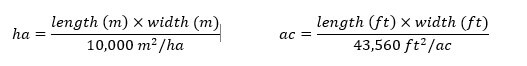
Step 1 – How large is the area you need to spray?
Multiply the length of the area you plan to spray times the width. If you are using metres, then divide the product by 10,000, which is the number of m2 in a hectare (ha). For feet and acres, divide by 43,560 which is the number of ft2 in an acre (ac):
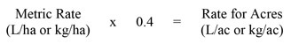
Step 2 – How much product is needed to spray the area?
Consult the rate(s) shown on the label. In Canada, rates are often based on planted area (E.g. hectares). In Australia and New Zealand, they may be based on row length (not covered in this article). If you measure your area in acres, you’ll have to convert the rate by multiplying by a constant: 0.4.
Now multiply the area you want to spray (step 1) by the rate (step 2).
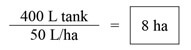
Step 3 – How far can you go on a full tank?
You know your sprayer output (determined through calibration) so you divide that into your tank size. Watch your units:
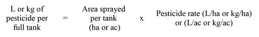
Step 4 – How much pesticide per tank?
Multiply the area that can be sprayed per tank (Step 3) by the pesticide rate (Step 2). Again, watch your units:
Step 5 – How much area is left to spray?
Just subtract what you’ve already sprayed from the total area.
Step 6 – How much pesticide in the last, partially-full tank?
Multiply the area you have left to spray (Step 5) by the pesticide rate (Step 2). Yes, watch your units:
Step 7 – How much spray mix will I need for the partial tank to finish spraying the total area?
Multiply the area you have left to spray (Step 5) by the sprayer output (determined through calibration). Guess what? Watch your units:
Sample problems
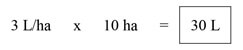
Time to test your knowledge. Let’s suppose you want to apply a product rate of 3 L/ha to your blueberries. You calibrate your sprayer and determine your output to be 50 L/ha. Your tank holds 400 L of spray mix. Your planting is 500 m long and 200 m wide.
Q1 – How large is the area you need to spray?
Q2 – How much product is needed to spray the area?
Q3- How much area can be sprayed on one tank?
Q4 – How much product should be added to a full tank?
Q5 – After the tank is empty, how much area is left to spray?
Q6 – How much product to add to the last, partially full tank?
Q7 – How much spray mix will be needed to finish spraying?
Exceptions
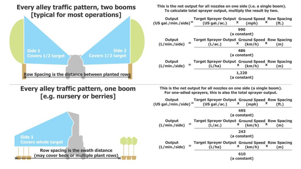
Certain situations aren’t covered in this article. If you are spraying a greenhouse, the math is different. If you are performing a banded application, the math is different. And, if you’re an airblast operator trying to reconcile why a pesticide label uses planted area rather than canopy volume for its rates, you’re in for a lot of additional reading. Some of that latter process can be summed up in this infographic:
When you find a method that works for you, write it down and keep it with your spray records. Happy spraying!
White mould is caused by the fungus Sclerotinia sclerotiorum and it’s an annual threat to soybean when cool, wet conditions correspond with flowering. Variety selection (e.g. high tolerance) and cultural control (e.g. crop rotation and wider row width) are important management tools, but ultimately the application of a crop protection product between R1 and R2 is required for high-risk fields. (Learn more here).
This article describes the results of an experiment exploring soybean canopy coverage and fungicide efficacy from a rotary spray drone. All work was performed under PMRA research authorization. There are currently no labels to apply crop protection products in Canada.
Experimental design
For the spray coverage trials, two locations were selected in southern Ontario (one south of Sparta and one west of Talbotville). This was a full field-scale trial with a single application made at R1.5 on July 18 (Sparta area) and July 22 (Talbotville area), 2023. There were two replications in each field and treatments were laid out parallel with the planting direction in a randomized design. Four other locations in Ontario and Quebec were also used in the larger efficacy/yield study. All locations had some level of white mould infection.
New Holland 345 – 150 L/ha (TeeJet XR11006 nozzles on 50 cm spacing) *Not included in spray coverage trial
We established an effective swath width of approximately 4 m (13.1 ft). The drone made three passes to cover the 12 m (40’)-wide treatment area, corresponding to the widths of the 9 m (30’) or 12 m (40’) headers later used to harvest in each field. Buffers were left on either side the treatment area. Fungicide was applied at label rate plus 0.125% Activate.
Target placement and retrieval
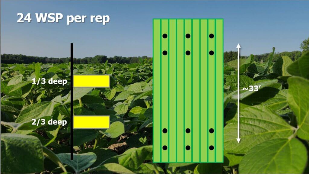
Soybeans were planted on 38 cm (15”) row spacing. The coverage sampling area was positioned in the middle of the treatment area. A length of rebar was positioned in-row and sheathed in PVC tubing. Two SpotOn brand water sensitive papers (WSP) from the same production run were secured face-up approximately 1/3 and 2/3 deep in the canopy. A block of six such samplers were positioned in a 3 x 2 grid (every third row and approximately 2 m apart in row). This block was then repeated 10 meters (33’) further into the block for a total 24 water sensitive papers per replicated treatment (see below).
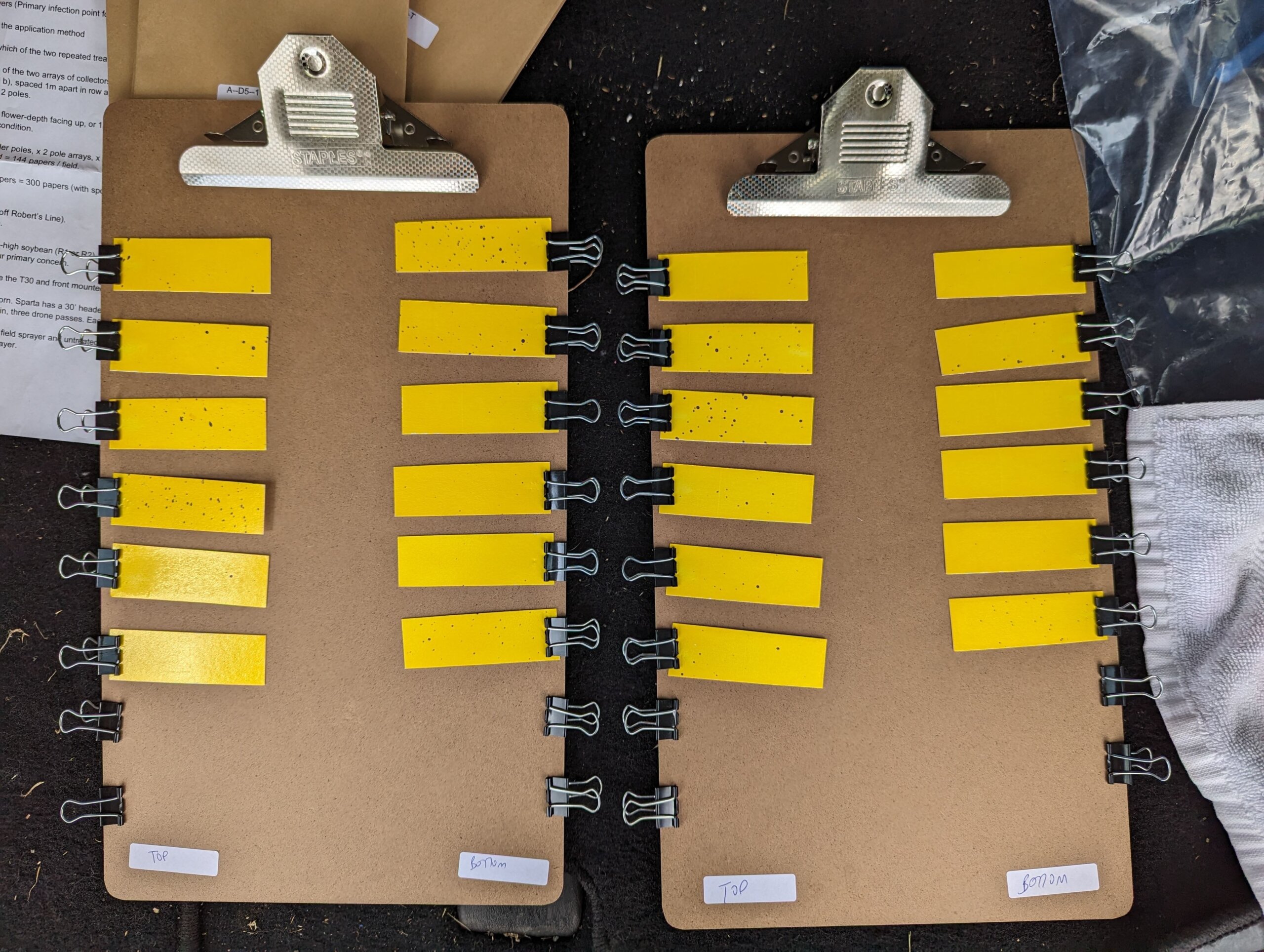
The papers were retrieved and temporarily placed on clipboards to dry before they were placed in paper bags for short term storage. They were digitized using a SprayX DropScope within 48 hours of retrieval on the “ground sprayer” setting, measured as percent surface covered (% area), and deposit density (# deposits/cm2).
Weather during coverage trials
Weather data was monitored using a Kestrel 3550AG weather meter (Kestrel Instruments) in a vane mount positioned 1.5 m (5 ft) above the ground. Wind speed fluctuated during the treatments, but wind direction remained relatively stable at 90 degrees to the flight path. The Sparta location averaged 6.4 km/h (4 mph) while the Talbotville location was considerably higher at 14.4 km/h (9 mph). Nevertheless, targets remained within the swath, despite any offset, as indicated by visual confirmation as well as the consistent coverage observed on the windward WSP compared to other, downwind samplers in each pass. Cloud cover was high at both locations.
Results
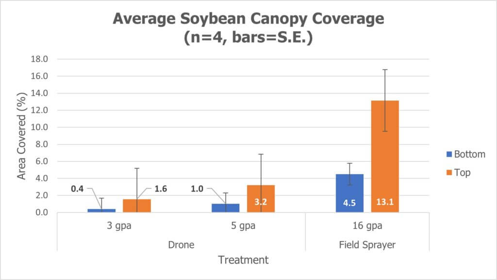
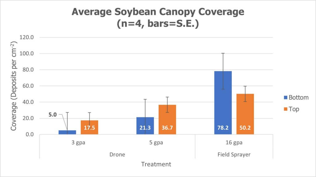
Coverage
The coverage recorded from each WSP was averaged by canopy position (bottom 1/3 or top 1/3 of canopy) and presented in the following histograms with standard error. There were some spoiled collectors, primarily in the lowest canopy position, ruined by high humidity and physical contact with the plant. However, the lowest n for any treatment was 31 collectors and the highest was the full 48. Coverage is presented both as % area covered and as deposit density in counts per cm2.
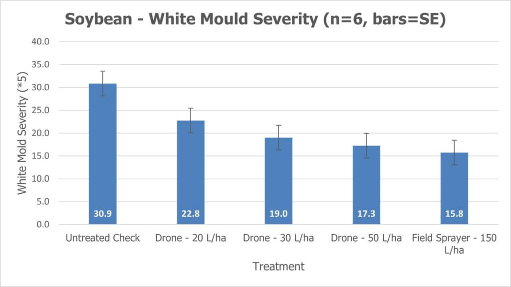
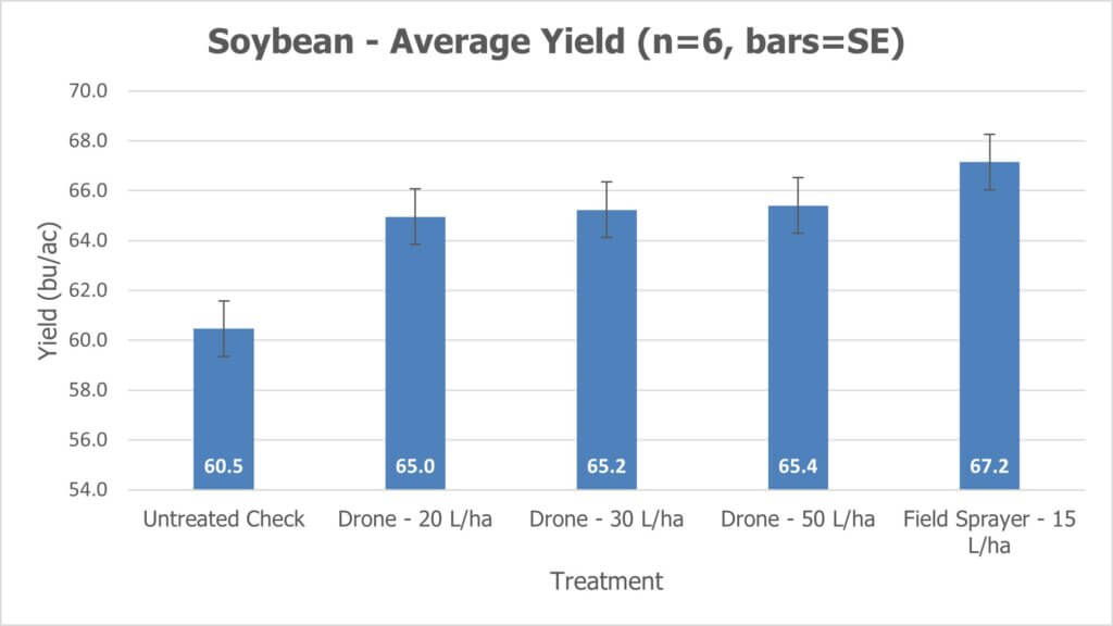
Efficacy and yield
Three phytotoxicity ratings were performed 7, 14 and 21 days after treatment. White mould was rated at harvest and final crop yield reported in bu/ac.
Observations and Considerations
As expected, both water volume and canopy depth share direct relationships with percent-area covered (i.e. lower water and lower canopy depths mean lower coverage). Water volume also shares a direct relationship with deposit density for a given droplet size, but canopy depth is more complicated as smaller droplets tend to penetrate more deeply into canopies and low water volumes tend to produce smaller droplets. However, as a general observation, less water translates to less coverage no matter the metric for coverage, and this has been shown to reduce product efficacy.
How, then, can we reconcile the claims of efficacy from low-volume drone applications? It’s typical that the % area covered from a 50 L/ha drone application is ¼ or less than that of “conventional” field drop systems which in North America tend to employ 150-200 L/ha. In speaking with Mark Ledebuhr (Application Insight LLC) about how low volumes could possibly be efficacious, he explained that in sugarcane production in Guatemala, the condensing humidity is likely the reason why their 1 gallon/acre applications are working. The droplet survivability, and the re-hydration and secondary movement of the deposits were a good thing.
In the case of contact fungicides in North America, it may be humidity as well, but also the deposit density, combined with higher concentrations of active ingredient, that explain the similar efficacy and yields as seen here between the 50 L/ha (drone) treatment and the 150 L/ha (field sprayer) treatment. This would concentrate both the active ingredient (possibly increasing uptake rate, or residue persistence, depending on the product mode of action and the target’s physiology) as well as the adjuvant load (possibly improving sticking/spreading of deposits).
Another consideration surrounds how deposit spread is analyzed. Water sensitive paper underestimates the spreading effect that can occur on plant surfaces (especially where surfactants are used). This is why WSP tends to be used as a relative index, meaning that papers should only be compared to other papers. Perhaps deposits are spreading more on the plant surfaces in the low-volume drone application (again, given the higher concentration of formulated adjuvants) than the water sensitive paper is indicating, and that is improving efficacy.
This concept of how low-volume applications might affect coverage and subsequent efficacy, and the potentially positive impact of re-formulating products to include higher adjuvant loads, is well-described in this precis by Dr. Andrew Chapple and Malcolm Faers. Currently, accepting that the amount of control provided by the drone application falls short of that provided by a field sprayer, this study indicates that drones have the potential to produce acceptable results in fungicide applications if conditions are suitable, timing is optimal and water volumes are sufficiently high.
This study was a collaborative effort with Bayer Canada and Drone Spray Canada.