Category: Speciality Sprayers

Main category for all sprayers that are not horizontal booms

  • Working with an Arborist: Drive-Along Diaries #1

    Working with an Arborist: Drive-Along Diaries #1

    April 23rd, 3:45 am

    I was excited. Today would be my first in a series of drive-along experiences with Ontario sprayer operators. However, to get from my home in Southwestern Ontario to Newmarket, I would have to cross Toronto. This is not my favourite thing to do. But, Dean Solway, Plant Healthcare Supervisor with Shady Lane Expert Tree Care, was based out of Mount Albert and he liked to start at 6:00 am. So, a hot shower and a hot coffee (not necessarily in that order) gave me the emotional support I needed to throw elbows on the parking lot we call the 401.

    It was strangely unsettling to see Tim Horton’s closed, and equally odd to see only a handful of cars on the highways. That may have been the fastest, smoothest drive through Toronto that I’ve ever had.

    5:45

    I arrived at the 10-acre lot that has been owned by the company for the last 45 years. I walked past a small, 500 tree nursery they’d recently planted to find Dean in the office. He was busy checking bookings for the day and assigning jobs to his three Plant Health Care trucks (PHC1, 2 and 3). More on those later. After a few introductions, I faded into the background and let them get on with things.

    Dean was ensuring the routes made sense and that everyone was ready to go. He explained that the week’s bookings were set each Friday, but that things could always change at the last minute. Front-line administration would handle client calls and communicate with the trucks throughout the day. They also ensured the clients were given at least a day’s notice that someone would be coming to treat their plants. Interestingly, the company is also required to inform the client’s neighbours. Dean said it helped avoid potential conflicts such cars, sunbathers or laundry left in the path of potential overspray. Not that such things ever happen, of course.

    Operators kept referring to “The Board” which showed their daily assignments. With 2,800 clients scatted over Brechin, Barrie, Oakville, Pickering, Oshawa and downtown Toronto, thoughtful planning and clear communication were critical requirements.

    I eavesdropped as Dean talked to a new hire about safety. Filter checks/replacements, face shields, gloves and orange vests were assigned, and I’m confident that it wasn’t staged for my benefit. Operator safety was a theme that came up throughout the day and it was clear Dean took it seriously. As the trucks got ready to roll, he fielded random questions about pesticide rates, tank mixes, crop staging and general agronomy as he double-checked that each truck was properly loaded.

    I learned that standard operating practice was to regularly test the equipment and plumbing in each truck. Experience showed it was easier and less contentious to deal with minor leaks and similar issues in the yard than on a Toronto highway or even worse, at a client’s home. That took us outside.

    6:15

    Each truck was equipped with a tablet containing SDSs for all the products they use, PDFs of the pesticide labels and a hyperlink to Health Canada’s Pesticide Label Search website. Many of the products used by arborists are biorational / organic, either by choice or because labels do not permit the use of many conventional pesticides in urban environments. I felt a bit of team-pride when I was told that OMAFRA’s Pub 840 is a significant reference document for the company.

    As he checked the trucks, Dean noted that it was important to explain to clients that eradicating pests isn’t always possible. Most often it’s about maintenance. For example, today would predominantly be about fungicide applications. Ornamental fruit trees such as crab apple were at risk of scab infection and the window for protection was narrow. Far be it for me to bring up climate change, but Dean did mention that this was the earliest he’d had to apply these products in nine years.

    Protectant fungicide treatments need time to dry to be effective. If it were to start raining steadily inside two hours following the application, Dean said the client would be eligible for a re-application ASAP. According to OMAFRA Publication 840, four applications were permitted for this chemistry, and clients were scheduled to receive three at regular intervals over four weeks. That gave time for the applicator to rotate back around, and it left capacity for a possible re-application if required.

    Incidentally, I am a master of foreshadowing.

    The Trucks

    PHC1 and PHC2 were designed to apply plant protection products. PHC3 was strictly for fertilizer and carried an extra 450 L just in case it was needed throughout the day. To remain flexible and efficient, the fertilizer applicators had to be able to take advantage of opportunities if the schedule changed. Returning to reload would be a big loss of productivity, so a little extra onboard was reasonable insurance.

    Dean explained that all the trucks were filled either the morning of, or the night before, depending on the product. In the case of compost tea, it’s a three-day process that requires a lot of planning. It must be applied at less than 50 psi to prevent mechanical damage to the living component of the mix. It can be applied to the soil or as a foliar treatment.

    We’d be riding in PHC1, which had a single tank subdivided into four separate 170-gallon tanks. The reel was a 60 amp electric auto reel with 300 feet of high-pressure hose. The pump was an AR 813 diaphragm pump, and the motor was a 20 hp twin cycle Vanguard and capable of producing up to 300 psi which is sometimes needed to reach the tops of the highest trees. Dean helped design this system himself and grinned when he said that even as low as 150 psi, you can feel the pistol “kick” in your hand.

    Speaking of which, the hose terminated in a quick-connect that allows the operator to swap between a pistol for nearby targets, and a long-barreled rifle for more distant targets. There was also a manually pressurized two gallon bottle sprayer for when the hose-and-gun assembly simply wouldn’t reach.

    The last thing Dean checked was that each truck had cleanup equipment, including detergents for any overspray accidents. He explained that most clients want no sign of the trucks coming, going, or having ever been there. That might mean washing away speckles on cars and windows, or marks from the hose being dragged on stonework or past beds and gardens. I’ll share my observations on how urban spraying seems to be viewed by the general public later on.

    6:45

    We’re on the road, passing through Newmarket in the York Region before slipping into stop-and-go traffic on the 404. We aren’t five minutes out before Dean’s phone rings. PHC1 is essentially his office, and he remains in communication via a work phone and headset, relying on a dedicated GPS to guide him from client to client… when the maps are accurate, anyway.

    As we drive, Dean notes that rain is forecast so we’ll do as much as we can. He’s set up a linear route going to the furthest client first and working our way back. That way, if it does rain, it will be easier to reschedule because the clients are closer to the yard. He also designs routes that keep the trucks in single neighbourhoods. It’s more efficient and jumping on and off the 407 is an expensive proposition, so they use it judiciously.

    7:40

    According to the docket, we were slated to spray two 12-foot Siberian Crab-apples in the client’s back yard. We pulled up and hopped out. Dean walked us to the back of the house saying, “Let’s go find our patients”. I liked that.

    The Process

    Once located, he assessed the trees’ health to ensure the application was appropriate, and then scanned the area. He explained that an arborist had to be very mindful of the surroundings. He ensured nothing was in the path of the hose or the spray, established wind direction, and then (based on tree height and our distance from the truck) estimated the pressure we’d need for the pistol attachment to reach to the treetops.

    We returned to the truck and Dean opened the side to put on his PPE. At the same time, he gave me a short safety lecture. Basically, if I saw anything leaking (on or under the truck) I was to turn off the engine immediately and we wouldn’t go anywhere until we figured out and remedied the issue. Also, should something happen to Dean, I was to call 911. Rest assured, there were no such issues that day.

    He ensured the pressure regulator was completely backed off, opened the intake and return valves on the fungicide tank, attached the pistol to the hose and started up the motor. Then he adjusted the regulator to get us to 150 psi. It was obvious he’d performed this dance many times and as he went through the motions, he noted that it was important to get comfortable with the equipment but to always be respectful of it. Then he partially-closed the side panel to reduce the motor noise and started dragging out enough hose to reach his patients.

    Standing upwind some distance away, I watched Dean work that first tree. He started with a few, short “test shots” into the ground to get the product to the pistol, and to adjust the width of the spray cone. Then a couple more test shots to the top of the tree to gauge the wind and the pressure. I watched him adjust the nozzle to a tighter stream and start circling the tree, spraying in short bursts until he was satisfied he’d achieved the coverage he was looking for.

    Then he detached and drained the pistol before starting back to the truck. I asked what kind of coverage he was looking for and he said the standard was 90% of the canopy covered by at least 90%. That was startling to me given that our unofficial goal for most dilute applications in perennial tender fruit, pome, cane and berry is 100% of the canopy covered, but to a minimum threshold of ~15%. It’s likely due to the different chemistries (I noted earlier that urban applications tend towards biorational products). And, practically speaking, airblast sprayer operators cannot slowly circle a tree, aiming at trouble spots with an endless volume of water. Despite these differences, both methodologies seem to produce acceptable results.

    The Label Dilemma

    I’ve always been sympathetic of sprayer operators working in three-dimensional crops. Interpreting a North American label’s frustrating lack of guidance when it comes to water volumes for non-arable crops places a lot on the operator’s shoulders. I’ve discussed this disconnect (and proposed solutions) in several other articles. I’ve even co-written a book about it. The problem was particularly acute, here.

    Ideally, one would evaluate the target tree’s planted area (which may or may not include an associated portion of alley) and work out the amount of formulated product required for that area. Then, that product must be dissolved or suspended in carrier (typically water) and that gives us the spray mix. Finally, working from the rate the sprayer emits, the operator would determine how much time would be needed to cover the target tree without over- or under-dosing. A good example of the process is found here.

    But… how much water is the right amount? How do we reconcile having to achieve such a high degree of coverage? Does that mean using a more dilute spray mix depending on the canopy, or the chemistry, or the method of application? And what happens when the target canopy size can be variable by an order of magnitude, such as going from a small, sparse tree to a huge, full tree? Would the operator have to change concentrations for every job in order to have the right combination of water volume and chemistry to propel and deposit the product uniformly?

    There’s no easy answer. Yet I watched Dean deal with this problem at every job, working to keep as much spray on target and use only as much spray mix as required to meet his coverage threshold.

    Administration and Cleanup

    Back at the truck Dean shut off the pump and reeled in the hose through a hand-held rag to ensure the hose came back cleaned of anything it may have been dragged through. Overall, it took six minutes to complete the spray job, but then the clients came out to speak to Dean and that conversation lasted another 10. Client interaction / education is a big part of this job.

    By 8:10 Dean had posted a Notice of Service sign in the yard (which must stay there for 48 hours) and punched in the next address on the GPS. As we headed off, he said a big improvement in recent years is the ability to email a Notice of Service and send an invoice right from the client’s driveway, immediately following the service. What traditionally was a 1-2 week wait for payment is now less than a day. If requested, Dean could also write them out manually and leave them at the client’s door.

    8:25

    The next client had five weeping crab apples. These were low trees easily accessed by the roadside truck. Wind was light so low pressure was required. Dean noted that he takes the pressure off the pump between stops to relax the drive belt. He double checked that the pistol was empty and said the reason he drains it after each job was to prevent any possibility of puddles in the truck, on the road or in the client’s driveway. “Customers should never see puddles. It’s better for the environment and it’s professionalism.”

    There’s a lot of wash, rinse, repeat from here on, so I’ll only note anything unique to each spray job. In this case, I watched more closely to understand how Dean aimed. A stream of liquid can traverse a great distance without being deflected by wind, but it’s not the cloud of droplets we generally associate with spraying. I realized Dean was shattering that stream of liquid on the larger branches to create the droplets. That’s also why he occasional pulsed the spray by fluttering the trigger; Sometimes the distance warranted a longer throw (long stream shattering of a branch) and sometimes a series of short pulses (shorter throw and the spray broke up on its own). I watched him as he circled each tree, changing his vantage as required. It wasn’t as easy as he made it look, and he was fast.

    9:05

    This was a single, 20-foot high crab apple tree. Dean cranked it up to 225 psi and started with the pistol. Given the height, the wind was more of an issue, so he waited for lulls, using short pulses over short distances and holding the stream for longer distances. He widened the nozzle only when the wind was light and the target was particularly close, but eventually switched to the long gun to reach the treetop.

    10:10

    This time we were spraying a Magnolia tree. Dean inspected the flowers closely. This tree might bloom for 5-8 days and if the flowers are too open, the oil we would use in the treatment might damage them in high UV. Plus, the mechanical damage from the spray might knock them off. But the flowers were still closed enough for the preventative to be applied.

    You may have noticed that in this case we weren’t using the fungicide, but instead we’d protect the tree from scale using an oil. So how (I wondered) do we empty the pump and 300 feet of hose of fungicide and exchange it for horticultural oil? Thanks to there being no physical or chemical incompatibility with these two products, it turned not to be the “big deal” it would be for most other spray operations.

    Dean opened the draw valve for the oil and kept the return valve open on the fungicide tank. Then he started the pump and hopped up on the truck to spray the fungicide right back into the fungicide tank. When he saw the spray turn opaque, he knew he had primed the oil and stopped spraying. Then he shut off the return on the fungicide tank and opened the return on the horticultural oil tank. The swap took almost no time at all and the subsequent treatment was a breeze.

    10:52

    Stop five was in Snowball Corners in King City and Dean was a little surprised that the work order underestimated the job. We expected a couple crab apples but instead found 20 trees far into a large backyard. Dean took some time with this new client to explain the process, then we fed all 300’ of hose out to reach the trees. We hoped there was enough in the tanks to finish the day!

    Winds were high, but there was nothing around and Dean used short bursts and a tight stream shattered on the trees themselves to reduce the number of driftable fines that would be produced by a wide spray. Slowly, picking his moments, he worked in the up-to-downwind direction so any overspray hit the next target.

    11:37

    One small Crabapple.

    12:00

    Nine ornamental apples.

    Interfacing with the Public

    I used to think that operations like vineyards and orchards, which often suffer the dreaded urban-rural interface, had the hardest time explaining crop protection to the public. And that’s not just agritourism operations with farmgate sales, either. Throughout the day, however, I elevated arborists to the top of the heap. Case in point:

    Before the trucks left that the yard that morning, one of the operators asked Dean about a job in downtown Toronto for a major business on Bloor Avenue. The client did not want applications performed after 8:00 am because hoses on sidewalks are a tripping hazard. They were also restricted from spraying at night because of city noise bylaws (those pumps can be loud).

    Accessing the plants can be very difficult and working in downtown Toronto can be exceptionally challenging. Dean knew the spot by rote, saying they should “Come from the street, look to 1 o’clock and 15 m from the statue to find the boxwoods. Then pace the distance to ensure the 300 foot hose would reach. If not, transfer the chemistry to bottle spray. If so, bring the operating pressure up to compensate for the distance.”

    Dean explained that the crew-leader of each truck makes the call for the most effective and safest set-up. He went on to relate stories about angry neighbours that responded poorly to seeing staff in PPE, or the grief they would suffer when a flower bed or stone path was marred by the hose. He reiterated throughout the day how much of his job was explaining the spray application process to clients, their neighbours and anyone (read everyone) that might be watching.

    Dean said there would always be a way forward if you gave it some thought. “Work the problem. Don’t let the problem work you.”

    12:33

    One backyard crabapple.

    1:10

    Two crab apples in the backyard. This was the last stop and it was perhaps the most complicated. One nearby tree was vibrating with honeybees. The wind was blowing into the neighbour’s yard and the two tall trees were on the property line. Dean really took his time here, rapidly pulsing the pistol whenever the wind died down and directed away from the pollinators. Some overspray moved to the next yard, but it couldn’t be helped. At least it was minimized. All in all we were pleased at the accuracy.

    Then the clients, who were new, came home and Dean once again spent time with them explaining the process. We got back in the truck after posting the sign and as Dean emailed the Notice of Service and the invoice, the first few drops of rain started to hit our windshield. All that patience and effort on the last stop and the client would likely need a re-application the next day. Dean was unflappable: “You can’t control the weather.”

    Epilogue

    We grabbed a late lunch and Dean drove us back to the yard. I’d learned a lot and really enjoyed Dean’s company. He headed back into the office to see how the day went for the other operators and plan for tomorrow. As for me, it had been a long day and I was loathing the punishing drive ahead of me… so I sprang for the 407 toll highway.

    Take Homes

    Upon reflection, and having written this article over about two weeks, I think I’ll end each article with a few observations. Bear in mind that I do so based on a sample size of one. That means what I did and what I saw may be unique; It should not be taken to represent an industry, a company, or even the typical practices of a single operator given that we only spent one day together.

    • Generally, label direction does not adequately inform sprayer operators working in three-dimensional crops. I have noted this in fruit protection systems and greenhouse systems, but it may be particularly relevant for arborists.
    • The classic urban-rural interface can cause friction between agricultural production and surrounding residential areas. Not only as a function of pesticide drift, but also noise, dust, odour, etc. Arborists work in urban environments, are scrutinized constantly and are quite often misunderstood by well-meaning people. As such, their job is far more than product application – they spend a considerable amount of time educating and answering questions, making them front-line ambassadors for crop protection processes.
    • The concept of threshold spray coverage (or minimal effective dose) continues to be a difficult and elusive thing. Factors such as mode of action, the nature of the target (surface structure and location), environmental conditions, application equipment and spray quality/concentration are already tricky to say the least. Having watched the relatively dilute, saturating, and highly mechanical applications performed by an arborist I continue to reassess what I think of as “good coverage”.
    • We sprayed 42 trees in roughly seven hours. Productivity, refill time, travel time and the economic considerations common to all spraying have different standards in each agricultural space. Efficiency is, obviously, important to any operation, but this experience reinforced just how different each operation can be. An orchardist may grumble about having to drive between blocks using county roads but imagine doing that on the 404! It’s all relative.

    Stay tuned for the next installment.
  • The Drive-Along Diaries: Prologue

    The Drive-Along Diaries: Prologue

    I feel it’s important to occasionally remind myself why I do what I do, and who I’m doing it for. With that, let me tell you a story.

    I was recently asked to give a presentation about spray coverage and drift mitigation to an arborist organization. I agreed but harboured reservations. I’ve given talks of this nature many, many times, but I rarely work with arborists. In preparation I looked back through my files and discovered I’d spoken to them 10 years ago. Coincidently, that was also the last time I’d encountered an arborist.

    So, what value could I possibly offer? My concern was that all I’d leave them with was a few “factoids” and the vague sense that they’d been entertained. But would I leave things better than I found them? What could I say that would move the needle and give them something actionable?

    Fortunately, I was paired with a veteran sprayer operator and together we worked out a presentation / demonstration. It went over very well, and I was relieved that people were engaged and asked insightful questions. Crisis averted.

    I believe the reason it worked was because I asked the operator about the real-world challenges (however unpopular) that he faced. We discussed and agreed upon a few lesser-of-two-evils solutions to share with the group. It was authentic, it was pragmatic, and it was appreciated.

    As a result, I decided to dedicate some time this spring/summer to riding along with a variety of sprayer operators as they perform their jobs. If they’d have me, I’d promise to stay out of their hair, acting only as an observer. I wouldn’t make suggestions and I wouldn’t criticize. I would ask the occasional question and I’d watch to see where policy and reality crossed paths.

    I was hoping for a few educational experiences that would inform my research trajectory and teach me a few tips and tricks to share at winter meetings. Perhaps I’d reinforce my understanding of spray application, or maybe I’d be forced to re-evaluate my position on what is a technical truth and what is a practical truth. At the very least I would get to see how professionals did their jobs, and which best practices got sacrificed when things didn’t go to plan.

    And, while I was at it, I decided to keep a journal to create articles in the vein of “A Day in the Life”. You’re reading the first one right now and I hope you find it as interesting to read about as I did to live it. It’s unlikely you work in all the agricultural spaces I’ll be writing about in this series but keep an open mind. The potential for cross-pollination is enormous; Perhaps your “cousin” sprayer operator has solved a problem you face in your own operation.

    And so, given our recent success, my first victim will be my new arborist-friend. You can read all about it here.

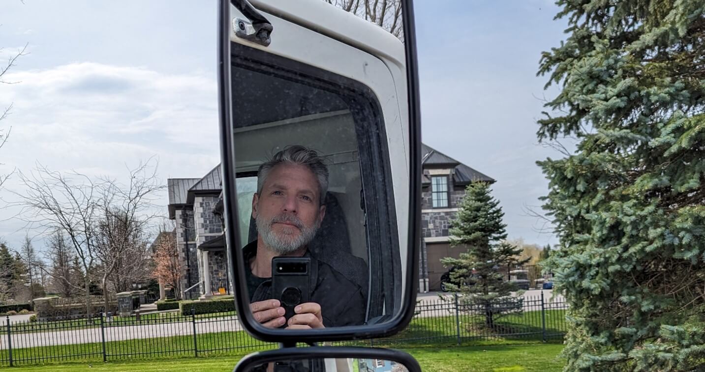
    A quick selfie in suburbia as I’m guided through a day in the life of an arborist.
  • Exploring Spray Drones in Soybean

    Exploring Spray Drones in Soybean

    White mould is caused by the fungus Sclerotinia sclerotiorum and it’s an annual threat to soybean when cool, wet conditions correspond with flowering. Variety selection (e.g. high tolerance) and cultural control (e.g. crop rotation and wider row width) are important management tools, but ultimately the application of a crop protection product between R1 and R2 is required for high-risk fields. (Learn more here).

    This article describes the results of an experiment exploring soybean canopy coverage and fungicide efficacy from a rotary spray drone. All work was performed under PMRA research authorization. There are currently no labels to apply crop protection products in Canada.

    Experimental design

    For the spray coverage trials, two locations were selected in southern Ontario (one south of Sparta and one west of Talbotville). This was a full field-scale trial with a single application made at R1.5 on July 18 (Sparta area) and July 22 (Talbotville area), 2023. There were two replications in each field and treatments were laid out parallel with the planting direction in a randomized design. Four other locations in Ontario and Quebec were also used in the larger efficacy/yield study. All locations had some level of white mould infection.

    1. Untreated Check
    2. *DJI Agras T30 – 20 L/ha (6.8 m/s, 2.5 m above canopy, TJ TT110015)
    3. DJI Agras T30 – 30 L/ha (5.7 m/s, 2.5 m above canopy, TJ TT110015)
    4. DJI Agras T30 – 50 L/ha (3.3 m/s, 2.5 m above canopy, TJ TT110015)
    5. New Holland 345 – 150 L/ha (TeeJet XR11006 nozzles on 50 cm spacing)
      *Not included in spray coverage trial

    We established an effective swath width of approximately 4 m (13.1 ft). The drone made three passes to cover the 12 m (40’)-wide treatment area, corresponding to the widths of the 9 m (30’) or 12 m (40’) headers later used to harvest in each field. Buffers were left on either side the treatment area. Fungicide was applied at label rate plus 0.125% Activate.

    Target placement and retrieval

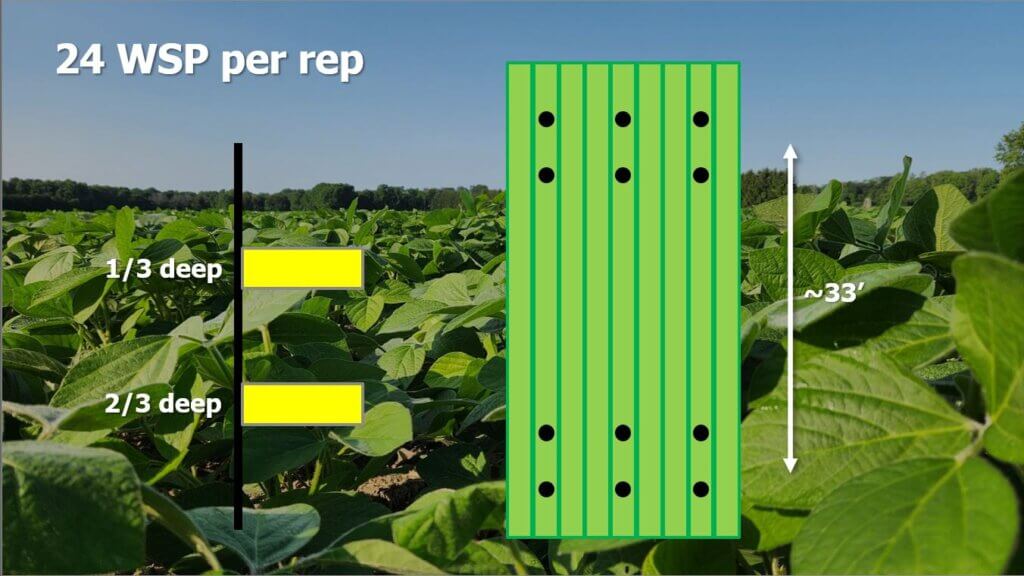
    Soybeans were planted on 38 cm (15”) row spacing. The coverage sampling area was positioned in the middle of the treatment area. A length of rebar was positioned in-row and sheathed in PVC tubing. Two SpotOn brand water sensitive papers (WSP) from the same production run were secured face-up approximately 1/3 and 2/3 deep in the canopy. A block of six such samplers were positioned in a 3 x 2 grid (every third row and approximately 2 m apart in row). This block was then repeated 10 meters (33’) further into the block for a total 24 water sensitive papers per replicated treatment (see below).

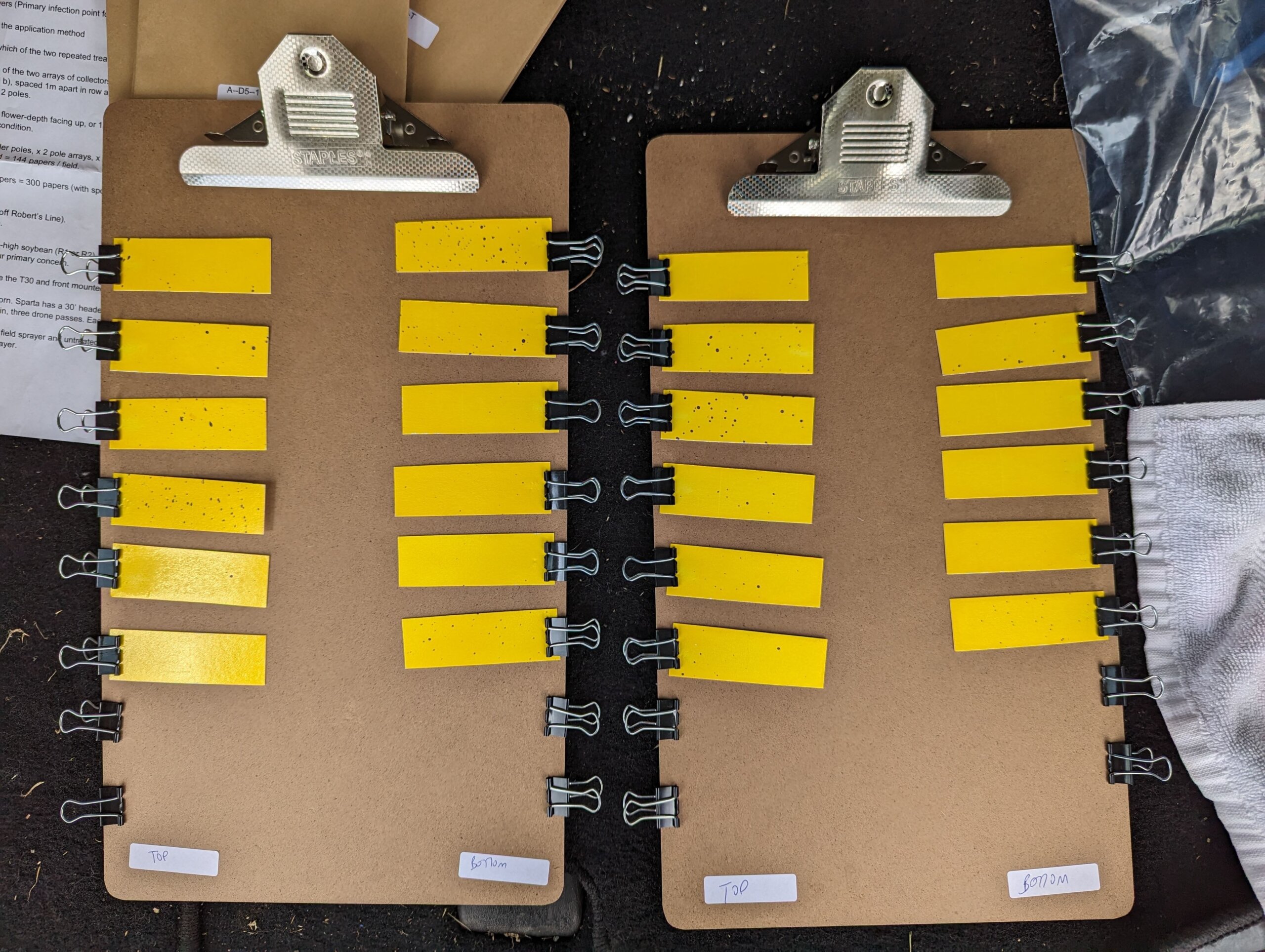
    The papers were retrieved and temporarily placed on clipboards to dry before they were placed in paper bags for short term storage. They were digitized using a SprayX DropScope within 48 hours of retrieval on the “ground sprayer” setting, measured as percent surface covered (% area), and deposit density (# deposits/cm2).

    Weather during coverage trials

    Weather data was monitored using a Kestrel 3550AG weather meter (Kestrel Instruments) in a vane mount positioned 1.5 m (5 ft) above the ground. Wind speed fluctuated during the treatments, but wind direction remained relatively stable at 90 degrees to the flight path. The Sparta location averaged 6.4 km/h (4 mph) while the Talbotville location was considerably higher at 14.4 km/h (9 mph). Nevertheless, targets remained within the swath, despite any offset, as indicated by visual confirmation as well as the consistent coverage observed on the windward WSP compared to other, downwind samplers in each pass. Cloud cover was high at both locations.

    Results

    Coverage

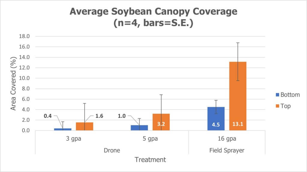
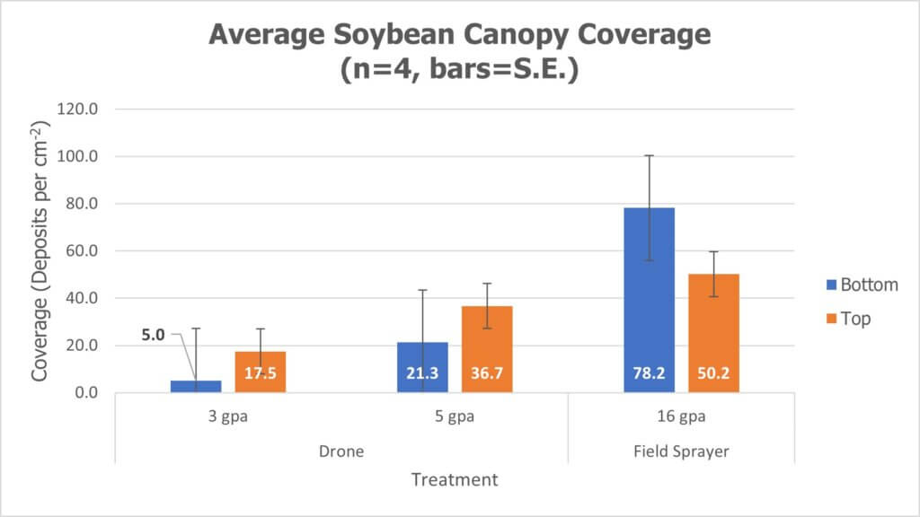
    The coverage recorded from each WSP was averaged by canopy position (bottom 1/3 or top 1/3 of canopy) and presented in the following histograms with standard error. There were some spoiled collectors, primarily in the lowest canopy position, ruined by high humidity and physical contact with the plant. However, the lowest n for any treatment was 31 collectors and the highest was the full 48. Coverage is presented both as % area covered and as deposit density in counts per cm2.

    Efficacy and yield

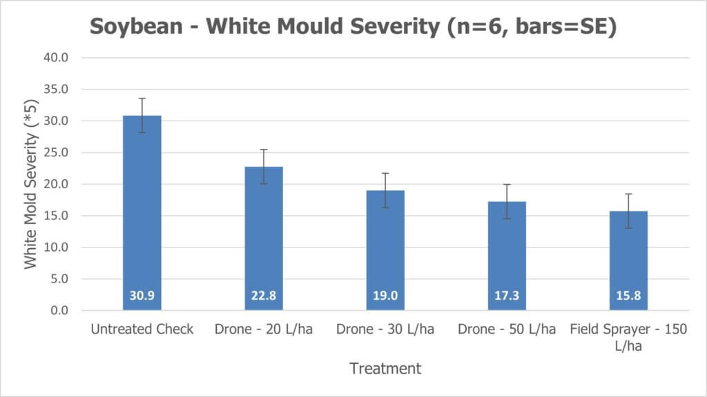
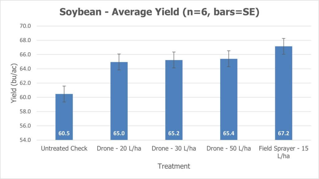
    Three phytotoxicity ratings were performed 7, 14 and 21 days after treatment. White mould was rated at harvest and final crop yield reported in bu/ac.

    Observations and Considerations

    As expected, both water volume and canopy depth share direct relationships with percent-area covered (i.e. lower water and lower canopy depths mean lower coverage). Water volume also shares a direct relationship with deposit density for a given droplet size, but canopy depth is more complicated as smaller droplets tend to penetrate more deeply into canopies and low water volumes tend to produce smaller droplets. However, as a general observation, less water translates to less coverage no matter the metric for coverage, and this has been shown to reduce product efficacy.

    How, then, can we reconcile the claims of efficacy from low-volume drone applications? It’s typical that the % area covered from a 50 L/ha drone application is ¼ or less than that of “conventional” field drop systems which in North America tend to employ 150-200 L/ha. In speaking with Mark Ledebuhr (Application Insight LLC) about how low volumes could possibly be efficacious, he explained that in sugarcane production in Guatemala, the condensing humidity is likely the reason why their 1 gallon/acre applications are working. The droplet survivability, and the re-hydration and secondary movement of the deposits were a good thing.

    In the case of contact fungicides in North America, it may be humidity as well, but also the deposit density, combined with higher concentrations of active ingredient, that explain the similar efficacy and yields as seen here between the 50 L/ha (drone) treatment and the 150 L/ha (field sprayer) treatment. This would concentrate both the active ingredient (possibly increasing uptake rate, or residue persistence, depending on the product mode of action and the target’s physiology) as well as the adjuvant load (possibly improving sticking/spreading of deposits).

    Another consideration surrounds how deposit spread is analyzed. Water sensitive paper underestimates the spreading effect that can occur on plant surfaces (especially where surfactants are used). This is why WSP tends to be used as a relative index, meaning that papers should only be compared to other papers. Perhaps deposits are spreading more on the plant surfaces in the low-volume drone application (again, given the higher concentration of formulated adjuvants) than the water sensitive paper is indicating, and that is improving efficacy.

    This concept of how low-volume applications might affect coverage and subsequent efficacy, and the potentially positive impact of re-formulating products to include higher adjuvant loads, is well-described in this precis by Dr. Andrew Chapple and Malcolm Faers. Currently, accepting that the amount of control provided by the drone application falls short of that provided by a field sprayer, this study indicates that drones have the potential to produce acceptable results in fungicide applications if conditions are suitable, timing is optimal and water volumes are sufficiently high.

    This study was a collaborative effort with Bayer Canada and Drone Spray Canada.

  • How to Succeed with a Soil Drench Application in Strawberries

    How to Succeed with a Soil Drench Application in Strawberries

    In 2016, Ontario berry growers were surveyed to determine the typical spray volume they used to apply unspecified crop protection products. For strawberry growers (day-neutral and June-bearing), the results spanned 50 to 1,000 L/ha (~5 gpa to ~100 gpa). In an earlier survey (2013), respondents specified 250 to 650 L/ha (~26.5 to 70 gpa) for fungicides, herbicides and insecticides. Miticide applications were as high as 750 L/ha (80 gpa).

    This rather wide span of carrier volumes shouldn’t be surprising. No matter the horticultural cropping system, the choice of carrier volume reflects the operation’s unique pressures and priorities. These variables include, but aren’t limited to, operation size, spray equipment, crop varieties/staging, geography, and pest profiles. The ultimate goal is to achieve threshold coverage (i.e. efficacy) while maximizing productivity.

    However, even the highest carrier volume reported did not reach the volumes required for those crop protection products intended to drench the soil. These products can span a range of 1,200 to 2,000 L/ha (~128 to 214 gpa). Experienced matted-row strawberry growers employ different methods to apply soil drenches, and we will discuss them later in the article. But first let’s address three common factors that must be considered:

    Know the target

    If (for example) the target is white grubs in the root zone, or phytopthora root rot, then the spray should be focused at the base of the plant in a banded application. Performing a broadcast application that covers the alleys as well as the plant rows may represent wasted spray. Knowing the target can help make the most efficient use of carrier.

    Know the soil

    Soil that is compressed or has high clay content won’t soak up water as quickly as drier, looser or sandier soil. If the beds are raised and resist absorption, much of the volume will run off into the alleys. This may not be desirable if the target is the raised bed itself. The following basic water movement principles come from the Manitoba Agriculture, Food and Rural Initiatives Soil Management Guide.

    • Water flows more quickly through large pores (sandy soils) than small pores (clay soils); water is held more tightly in small pores (clay soils) than in large pores (sandy soils).
    • Water moves from wet areas to dry areas (not necessarily by gravity) due to forces of adhesion and cohesion. This is called matric flow.
    • Water will not move from small soil pores to large soil pores unless conditions are saturated.

    Know the weather forecast

    Spraying on a hot, dry day means a higher rate of evaporation. As the carrier evaporates, the product will have less opportunity to infiltrate the soil. Conversely, applying product just before a heavy rain can result in a much diluted product being rinsed too deeply into the soil and beyond the target area.

    Consider that one millimetre of rain on one hectare of land is 10,000 litres. That seems like a lot, but how deeply does it infiltrate into soil? One way to know is to use calculations based on soil porosity and bulk density. From these calculations it can be generalized that 25 mm of rain will infiltrate 45 mm into dry, sandy soil, but only 32 mm into dry clay soil. Remember, that 25 mm of rain represents 250,000 L/ha!

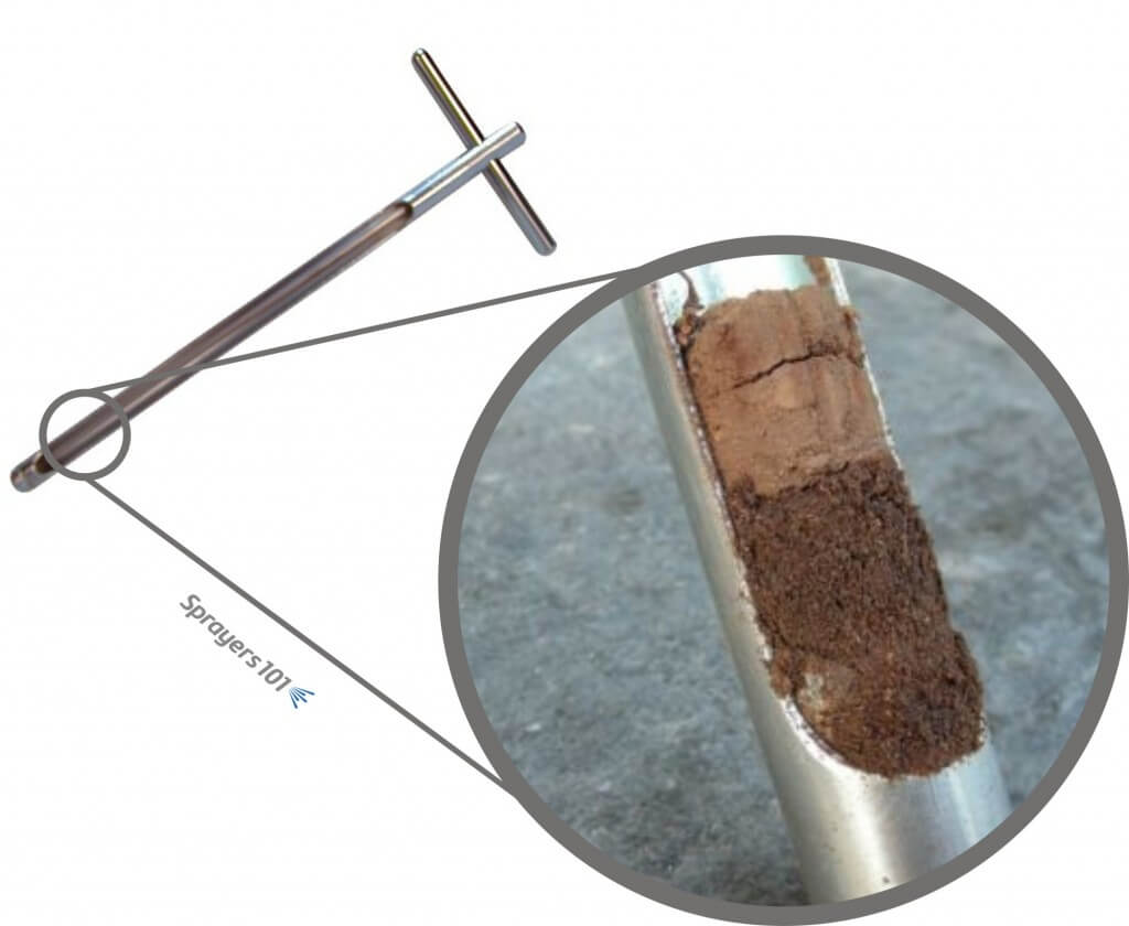
    Perhaps the best way to know how far water will infiltrate the soil is to use a soil probe (aka soil sample tube). They can be purchased from local dealers for about $100.00 CAD, or they could be borrowed from whomever provides soil sampling services in the area. For the best results, perform this test in multiple locations in the field.

    The soil probe. See how far water infiltrates soil by taking core samples.
    The soil probe. See how far water infiltrates soil by taking core samples.

    So what methods do strawberry growers employ to apply a drench? Here are the top three:

    1. Slow down

    Some growers elect to use their existing sprayer setup, but they slow down to get more volume on per hectare. For example, if the grower normally applies 500 L/ha (53.4 gpa) driving at 5 km/h (3.1 mph) they would have to drive 1.25 km/h (0.78 mph) to achieve the 2,000 L/ha some labels require. If the sprayer tank held 1,500 litres (~400 US gallons) that would mean doing 0.75 hectares (1.9 acres) to a tank compared to the normal 3 hectares (7.5 acres). That would be four times as long, without considering the time for the extra refills.

    Alternately, but related to slowing down, is double-pass spraying. In this case the tank is mixed at half-rate and the operator makes a pass through the field. Then, a second half-rate tank is applied immediately afterwards, ideally driving from the opposite direction. This effectively gives a full rate of product in a higher volume of water.

    2. Re-nozzle

    When slowing down is not enough (or not an option), some growers elect to re-nozzle. It may be tempting to increase the operating pressure to increase output on existing nozzles, but that makes finer droplets which tend to drift off target. The largest hollow-cone nozzles will only emit ~870 L/ha at 5.0 km/h (93 gpa at 3.1 mph) and that’s at 125 psi, which many trailed sprayers cannot manage. Further, many labels indicate a need for Coarse droplets in a drench, and hollow cones cannot produce such large droplets.

    There are a limited number of flat fan nozzles that can achieve sufficiently high rates, and even then they must be used at slightly slower travel speeds. For example, the TeeJet AI11008 used at 70 psi will apply 145 gpa (~ 1,350 L/ha) with a Very Coarse spray quality at 4 mph (6.4 km/h). Driving slower can rise those volumes considerably. Alternately, streamer nozzles (e.g. TeeJet’s 5 or 7 hole StreamJets) require lower pressures (up to 60 psi) to emit as much as 2,310 L/ha at 5.0 km/h (247 gpa at 3.1 mph). The grower can maintain their travel speed, but will still have to refill more often.

    3. “Wash In” the spray

    Still another choice is to apply the product using the existing sprayer set-up, using a typical carrier volume, just prior to a rain event or sprinkler (not drip line) irrigation. For example, if the grower normally applies 500 L/ha (53.5 gpa), they would continue to do so. If the grower is relying on rain to wash the product in, it should be sufficient precipitation to move the product to the desired soil depth. Where sprinklers are an option, this can be controlled, and the depth of infiltration tested with a soil probe. Washing in the spray should take place as soon after application as possible to ensure the product is distributed evenly into the soil.

    Thanks to Pam Fisher, former OMAFRA Berry Crop Specialist, and Anne Verhallen, former OMAFRA Soil Management Specialist, for their contributions to this article.

  • Rotary-Wing Drone Spray Coverage and Drift in Field Corn

    Rotary-Wing Drone Spray Coverage and Drift in Field Corn

    This work was performed with Mark Ledebuhr (Application Insight LLC.), Adrian Rivard (Drone Spray Canada) and Adam Pfeffer (Bayer Crop Science – funding partner). Amy Shi is gratefully acknowledged for her assistance with statistical analysis.

    Introduction

    In June 2017, Transport Canada cleared the general use of drones. In 2018, Health Canada clarified that the use of Remote Piloted Aircraft Systems (RPAS) for pesticide application is not permitted under the Pest Control Products Act without sufficient data to characterize any associated risk. Currently, there are no liquid pest control products registered for application by drone in Canada.

    Stakeholders want to use drones to apply pest control products in Canada. To that end, several research trials have been approved by Health Canada. However, multi-rotor drones represent a unique application technology more akin to air-assisted ground sprayers than manned aircraft. As such, conventional models for drift, exposure and efficacy may not apply. Fundamental questions surrounding the utility of drones must be addressed before efficacy and residue can be considered in any relevant context.

    Research and user experience has identified, and is beginning to understand the relative influence of, external factors such as crop morphology, planting architecture, topography, and environmental conditions. Considered with the product mode of action, these factors inform operational settings such as altitude, travel speed, nozzle choice, and application volume to optimize applications. This collective “Use Case” depends on drone design, which is highly variable and rapidly evolving.

    Having performed preliminary work characterizing effective swath width, and recognizing its popularity in North America, we used DJI’s Agras T10 in this study. Our objective was to evaluate fungicide efficacy on Northern Corn Leaf Blight, Tar Spot, Grey Spot and Common Rust in field corn, as applied using the T10. Drift and coverage would be characterized to provide context for the efficacy analysis, but also to develop data to inform best practices and possibly regulatory decisions surrounding risk. Aspects of the study would be repeated using conventional ground sprayer technologies to form a basis for comparison.

    Objectives

    1. Quantify spray coverage in field corn at three canopy depths, on adaxial and abaxial surfaces, as recovered tracer dye (indexed to % of applied rate ac-1), area covered (%) and deposit density (deposits cm-2).
    2. Quantify drift as recovered tracer dye (indexed to % applied rate ac-1) collected using the horizontal flux method up to eight meters high on the immediate downwind edge of the application.
    3. Evaluate the fungicide efficacy, applied using the T10, at 2 and 5 gpa as compared to a conventional overhead broadcast treatment at 16.7 gpa.

    Material and Methods

    Design

    Trials were conducted between July and August of 2022 in three Ontario corn fields. The locations, the application methods and data collected are detailed in Table 1.

    FieldLocationCorn VarietyApplication MethodRate (gpa)Data Collected
    1Jaffa (42°45’56.6″N 81°02’06.5″W)DKC45-65RIBAgras T102 and 5Drift, Coverage, Efficacy
    Overhead Broadcast16.7Coverage, Efficacy
    2Fingal (42°42’17.9″N 81°15’15.3″W)DKC49-09RIBAgras T102 and 5Drift, Coverage, Efficacy
    Overhead Broadcast16.7Efficacy
    3Port Rowan
    (42°35’53.6″N 80°30’43.2″W)
    P0720AMDirected (Drop hoses)20Coverage
    Table 1 – Trial sites by application method and data collected

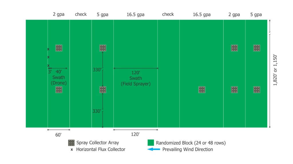
    Treatments were arranged in a randomized complete block design (Figure 1). Corn was planted on 30″ centres, with about 6” in-row spacing between stalks. We targeted spray for the R1 stage of development (approx. 8’ high). Fields 1 and 2 each hosted two replicated treatments of 2 gpa, 5 gpa, and 16.7 gpa, as well as two unsprayed checks. In field 1, blocks were 60’ (24 rows) wide by 1,150’ long for the T10, and 120’ (48 rows wide) by 1,150’ long for the broadcast field sprayers. A single, 120’ swath was applied using the field sprayers, and four 10’ (4 row) swaths were required to spray the centre 40’ (16 rows) of corn using the T10. This was based on a 10’ effective swath width determined in previous research. Field 2 had a similar layout but was 1,820’ long.

    Figure 1- Sample experimental layout for Field 2. In this example, horizontal flux collectors are positioned 3’ downwind to intercept any off-target drift from the edge of the adjacent 2 gpa treated area.

    Coverage Analysis

    To account for variability, each treatment block was subdivided into two regions, each containing an array of nine spray collectors. Each spray collector (Figure 2) consisted of a vertical, 8’ pole in-row between corn plants. Samplers were attached at three depths to span the silking region: Top: 1.5’-2’ below the tassel. Bottom: 1.5’-2’ from the ground. Middle: halfway between them. Samplers were parallel with the ground to ensure the highest degree of spray interception. On one side, two 1”x3” water sensitive papers (WSP; Innoquest Inc.) were clipped back-to-back with a sensitive side positioned up (adaxial) and facing down (abaxial). The other clip held two 4” square sheets of Mylar in the same orientation. Sampler type was alternated vertically (e.g. Mylar – WSP – Mylar or WSP – Mylar – WSP).

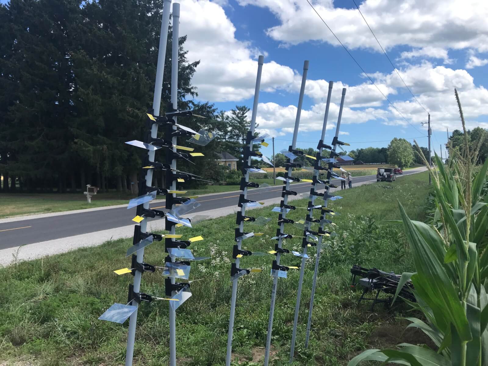
    Figure 2- Spray collectors temporarily loaded with WSP and Mylar samplers. These were held above the tassels as they were carried to the collection sites in each block. Three clips were positioned per pole, alternating Mylar and WSP samplers on each side, on two arrays of nine poles, as previously described.

    This study used 864 WSP and 864 Mylar samplers for the RPAS treatments, and 162 WSP for the overhead broadcast and directed applications. Following the application, samplers were retrieved as soon as they were dry enough to handle (about 30 minutes) and individually placed into pre-labeled sealable plastic bags, each uniquely coded to the exact position and orientation of the collector.

    Operational Use Cases

    • 5 gpa: DJI Agras T10 was operated at 3.3 m/s, 2 m above tassels. TeeJet 11002 AIXR nozzles equipped with 50 mesh filters were operated at 70 psi.
    • 2 gpa: DJI Agras T10 was operated at 7.0 m/s, 2 m above tassels. TeeJet 11002 AIXR nozzles equipped with 50 mesh filters were operated at 45 psi.
    • 16.7 gpa: Overhead broadcast condition. Field 1 ran a John Deere 4038R operated at approx. 10 mph with TeeJet XR11006 nozzles on 20” spacing. Pulse width modulation (ExactApply) was engaged. Field 2 ran a New Holland 345 front-mounted boom sprayer with TeeJet XR11006 nozzles on 20” spacing.
    • 20 gpa: Directed condition. John Deere R4038 operated at approx. 4.5 mph with Beluga drop hoses suspended on 30” centres to correspond with alley spacing. Two nozzle bodies were positioned 15″ apart equipped with Greenleaf Spray Max 110015 nozzles to span the silking area.

    Drift Analysis

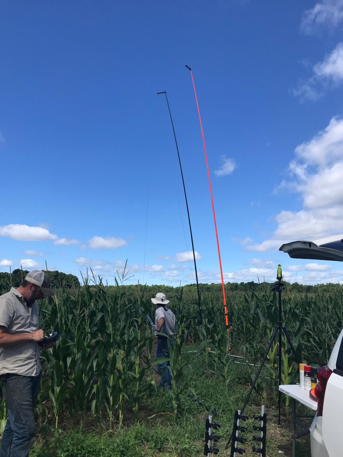
    Three free-standing 26’ (8 m) horizontal flux collectors were positioned in the corn field approximately 3’, or 1.5 rows from the downwind edge of the spray plot downwind of the area treated by drone (Figure 3). The sampling poles were positioned about 30’ apart parallel to the treatment block. Sterilized, 1.8 mm braided polyethylene collector line was run up the poles on pulleys just prior to application. Following applications, the line was collected in 1 m lengths into sealed bags.

    The assumption was that by placing the horizontal flux samplers as close to the “zero” downwind edge position as possible, nearly the entire off-swath movement of drift would be captured. A compromise of placing the samplers in the middle of the first row past the downwind swath edge was made due to the scale of the sample and the relative low swath precision of the drone. Placing the samplers closer to the zero downwind line was deemed to be too high a risk of inadvertently sampling in-swath.

    Figure 3- Moving horizontal flux poles into the field prior to positioning them for trials. String collectors were run up the poles just before spray application and retrieved immediately afterwards.

    Spray Solution (Formulated Product plus Tracer)

    Fungicide was applied at field rates (8 oz/ac or 586 mL/ha). The field sprayer applied this at 16.7 gpa. The drone applied it at 2 or 5 gpa but also included tracer solution at 0.2% (20 ml/10L solution) vol./vol. of a 20% mass/mass solution of PTSA in dH2O. PTSA residue data assumes 100% recovery and 0% degradation of the tracer. Tests of PTSA with fungicide prior to the study showed no physical antagonism and >98% tracer recovery. Prior testing of PTSA showed an acceptable 1-2% solar degradation in the timeframe required to collect samplers. Tank samples were drawn from the drone at the beginning and end of each trial and used to confirm tank concentration and to establish fluorescence curves.

    Weather Conditions

    Weather data was collected using a Kestrel 3550AG weather meter (Kestrel Instruments) in a vane mount positioned 1 m above the tassel (approximately 1 m below drone altitude). Data was logged every 5 seconds. Issues with data loss required us to supplement local data with Field Level Weather Summary data (Table 2).

    Date (2022)FieldVol. (gpa)Avg. Temp. (°C)Avg. Windspeed (km/h)Start TimeDuration (min.)
    Jul 2515*22.36.213:0035
    Jul 251521.47.518:4535
    Jul 26116.718.85.410:0045
    Jul 261223.97.715:3025
    Jul 2925**n/a16.411:0035
    Jul 2922***23.621.014:0025
    Aug 12320****25.46.313:3015
    Table 2- Date, location, and weather conditions for each treatment
    *Trial pass over spray collectors only – no horizontal flux collectors employed.
    **All bottom-level water sensitive paper samplers spoiled by high humidity. Wind changeable and horizontal flux poles moved 2x before application to orient downwind.
    ***Noted flocculation in tank samples likely from rainfastness adjuvant. Did not affect analysis.
    ****Coverage data from a single array of nine spray collectors with water sensitive paper samplers.

    Results

    Statistics

    The % applied rate ac-1, % area covered, and deposits cm-2 were subjected to analysis of variance using SAS® OnDemand for Academics PROC GLM. When a significant treatment effect was found, means were compared using Tukey’s honest significant difference test (HSD) at p=0.05.

    Data Collation

    Each spray collector was a vertical structure that supported Mylar samplers at three depths. Each depth held two samplers oriented abaxially or adaxially, in parallel with the ground. When discussing the amount of PTSA recovered by sampler depth or by sampler orientation, the % applied rate ac-1 of each of the nine related samplers were averaged within each array (n=2 arrays per block times two replicates equal n=4 per treatment).

    When considered from above, the six Mylar samplers are vertical cross-sections of the same area of ground. Therefore, the % applied rate ac-1 from each sampler was added to represent the total mass of tracer intercepted per collector. When these nine sub-samples are averaged, we arrive at the average % applied rate ac-1 per array.

    Similarly, the % applied rate ac-1 from each 1 m length of string on a horizontal flux collector could be averaged across collectors by relative position to explore drift by height (n=3 poles per block times two replicates equal n=6 per treatment). Alternately, the total PTSA recovered per pole could be calculated (n=3 poles per block times two replicates equal n=6 per treatment). This interpretation allowed us to perform a mass balance accounting of residue in-canopy and as drift compared to the known applied rate ac-1.

    It was not possible to collate the data in this fashion for the WSP because it was not possible to index % area or deposits cm-2 on a 1”x3” area to a theoretical maximum. Therefore, we averaged the nine samplers within an array relative to their position and orientation (n=2 arrays per block times two replicates equal n=4 per treatment) or averaged the six samplers per collector prior to averaging all collectors in an array (n=2 arrays per block times two replicates equal n=4 per treatment).

    RPAS Coverage – Mylar Samplers

    There is a negative linear relationship (r2=0.997) between the depth of the sampler and the average % applied rate ac-1 (Table 3). The deeper the sampler, the less tracer recovered. The sum of the average % applied rate ac-1 at each depth was 17.7% of known rate applied rate ac-1.

    Sampler DepthAvg. % Applied Rate ac-1Significance
    Top9.6A
    Middle5.7B
    Bottom2.4C
    Total:17.7
    Table 3- The depth of the sampler had a significant effect on the overall average amount of PTSA recovered.

    The orientation of the sampler significantly affected the overall average amount of tracer recovered (Table 4). The abaxial surfaces intercepted an average 11.1 % applied rate ac-1 less (a 97% difference) than adaxial surfaces. Note: When Mylar was retrieved a few had physically shifted, potentially exposing the back side of abaxial collectors to primary deposition from above. Therefore, it is assumed that the actual deposit is lower than reported here.

    Sampler OrientationAvg. % Applied Rate ac-1Significance
    Adaxial11.4A
    Abaxial0.3B
    Table 4- The orientation of the sampler had a significant effect on the overall average amount of PTSA recovered.

    When we separate the data to focus on the volume applied, we see volume had a significant impact on the amount of tracer recovered (Table 5). The average % applied rate ac-1 was 2.1% less (a 58% difference) in the 2 gpa condition compared to the 5 gpa condition.

    FieldAvg. % Applied Rate ac-1Significance
    17.1A
    24.6B
    Table 5- The field location had a significant impact on the average amount of PTSA recovered.

    When we isolate the volume applied by field, the 2 gpa treatment resulted in less coverage in field 2 (average 1.4 % applied rate ac-1 or 28% less) and significantly for the 5 gpa treatment (average 3.6 % applied rate ac-1 or 41% less: Table 6).

    DateFieldVolume (gpa)Avg. % Applied Rate ac-1Significance
    Jul 25159.2A
    Jul 26125.0B
    Jul 29255.6C
    Jul 29223.6B
    Table 6- The average amount of PTSA recovered by date and location show lower overall recovery in Field 2.

    When sampler depth is included in the field analysis (Table 7), we see similar deposition patterns; a negative linear relationship between coverage and canopy depth in all treatments save the 5 gpa treatment in field 2. Closer inspection confirms a reduction in coverage for the 2 gpa condition in field 2 versus field 1, and a significant reduction for the 5 gpa condition in field 2 versus field 1.

    Sampler DepthField 1 – Jul 25: 5 gpa.
    Avg. % Applied Rate ac-1 (Sig.)
    Field 1 – Jul 26: 2 gpa.
    Avg. % Applied Rate ac-1 (Sig.)
    Field 2 – Jul 25: 5 gpa.
    Avg. % Applied Rate ac-1 (Sig.)
    Field 2 – Jul 29: 2 gpa.
    Avg. % Applied Rate ac-1 (Sig.)
    Top15.2 (A)8.3 (A)8.0 (A)6.7 (A)
    Middle9.1 (B)4.7 (B)6.1 (AB)2.9 (B)
    Bottom3.5 (B)1.9 (C)2.6 (B)1.5 (B)
    Total:27.814.916.711.1
    Table 7- The average residue recovered by date, location and sampler depth is significantly less in the 5 gpa condition in field 2 and does not distribute linearly by sampler depth.

    RPAS Drift – Horizontal Flux

    Overall, the volume applied had a significant impact on drift, where the 2 gpa treatment resulted in an average increase of 1.6 % applied rate ac-1 (44% difference: Table 8) versus the 5 gpa treatment.

    Volume Applied (gpa)Avg. % Applied Rate ac-1Significance
    23.6A
    52.0B
    Table 8- The volume applied had a significant impact on the amount of the PTSA recovered.

    As with the Mylar samplers, there was a “field effect” where the field had a statistically significant impact on the amount of tracer recovered (Table 9). However, unlike the Mylar samplers in the crop, more tracer was recovered in field 2 (average increase of 3.2 applied rate ac-1 or a 67% difference) than in field 1.

    FieldAvg. % Applied Rate ac-1Significance
    11.4A
    24.2B
    Table 9- The field location had a significant impact on the amount of PTSA recovered.

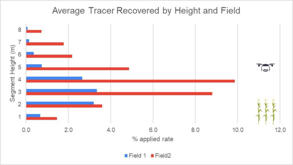
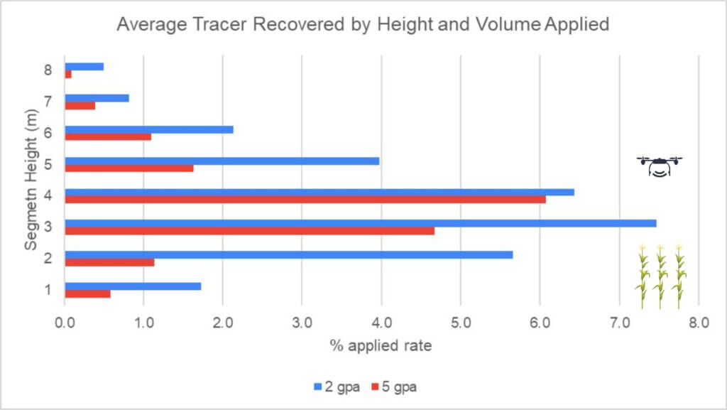
    The pattern of deposition by height was similar across all treatments. For context, note that the first 2.5-3 m of string were within the corn canopy and drone altitude was approximately 5 m off the ground (2 m over the tassels) per Figure 4 and 5. The differences were only statistically significant in field 2 (Table 10) where an average 33% applied rate ac-1 was intercepted compared to 11% in field 1.

    Figure 4- Average PTSA recovered (% applied rate ac-1) by height and field.
    Figure 5- Average PTSA recovered (% applied rate ac-1) by height and volume applied.
    Height
    (1m segment in m from ground)
    Field 1:
    Avg. % Applied Rate ac-1
    Sig.Field 2:
    Avg. % Applied Rate ac-1
    Sig.
    80.7A1.5C
    73.2A3.6BC
    63.3A8.8A
    52.7A9.9A
    40.7A4.9AB
    30.4A2.2BC
    20.1A1.8C
    10.1A0.7C
    Total:11.233.3
    Table 10- The average amount of PTSA recovered by height for field 1 and field 2.

    The volume applied had a significant effect on the total PTSA tracer detected in both fields, with an average 4.4% applied rate ac-1 more (a 59% difference) recovered in the 2 gpa treatment (Table 11 and Figure 5). Separated by fields, the 5 gpa treatment had an average 1.4% % applied rate ac-1 more (a 77% difference) in field 2 and the 2 gpa treatment had an average 2.8% % applied rate ac-1 more (a 76% difference) in field 2.

    Volume Applied (gpa)Field 1:
    Avg. % Applied Rate ac-1
    Sig.Field 2:
    Avg. % Applied Rate ac-1
    Sig.
    22.2A5.0A
    50.7B2.1B
    Table 11- The volume applied had a significant impact on the amount of PTSA recovered.

    Mass Balance Accounting

    It is never possible to entirely “close mass” in spray studies because there are other surfaces (e.g. leaves) within the vertical profile that intercept spray, as well as off-swath deposition and the ground itself (not measured in this study). Nevertheless, the exercise does allow us to estimate and compare how much spray was captured and how much remains unaccounted for (Table 12). We see that the 2 gpa treatment in field 1 had the highest unaccounted-for fraction, and on average we were able to account for an average 53% of the applied rate ac-1 in this study.

    Field
    (Volume in gpa)
    Coverage:
    Avg % Applied Rate ac-1
    (A)
    Drift:
    Avg % Applied Rate ac-1
    (B)
    Total % Detected
    (A+B)
    Unaccounted Fraction
    [100-(A+B)]
    1 (5)5155644
    1 (2)26.51743.556.5
    2 (5)30245446
    2 (5)19.54059.540.5
    Table 12- Closing mass using % PTSA detected on in-canopy samplers and on drift collectors.

    RPAS and ground rig coverage – Water Sensitive Paper

    The depth of the sampler had a significant effect on the overall average % area covered at all depths (Table 13). However, there was no significant difference at the two lower depths for deposit density (Table 14). In both cases, the negative linear relationship between coverage and sampler depth corresponds closely to the PTSA recovered on the Mylar samplers (see Table 3).

    Sampler DepthAvg. Coverage (% Area)Significance
    Top2.80A
    Middle1.28B
    Bottom0.62C
    Table 13- Overall average % coverage by sampler depth.
    Sampler DepthAvg. Coverage (Deposits cm-2)Significance
    Top44.5A
    Middle17.9B
    Bottom7.2C
    Table 14- Overall average deposit density by sampler depth.

    The sampler orientation had a significant effect on both overall average % area covered (Table 15) and deposits cm‑2 (Table 16).

    Sampler OrientationAvg. Coverage (% Area)Significance
    Adaxial3.03A
    Abaxial0.12B
    Table 15- The orientation of the sampler had a significant effect on the average % area covered.
    Sampler OrientationAvg. Coverage (Deposits cm-2)Significance
    Adaxial43.5A
    Abaxial3.1B
    Table 16- The orientation of the sampler had a significant effect on the average deposit density.

    The treatment had a significant effect on the overall % coverage (Table 17) with the overhead broadcast condition covering an average 3.31% more sampler surface (a 60% difference) compared to the next highest treatment value. The directed application delivered a significantly higher 67 deposits cm-2 (a 72% difference) compared to the next highest treatment value (Table 18).

    Treatment (gpa)Avg. Coverage (% Area)Significance
    Broadcast (16.7)5.91A
    Directed (20)2.32B
    Drone (5)1.34BC
    Drone (2)0.55C
    Table 17- Overall average % coverage by treatment.
    Treatment (gpa)Avg. Coverage (Deposits cm-2)Significance
    Broadcast (16.7)92.6A
    Directed (20)25.8B
    Drone (5)22.9B
    Drone (2)5.9B
    Table 18- Overall average deposit density by treatment.

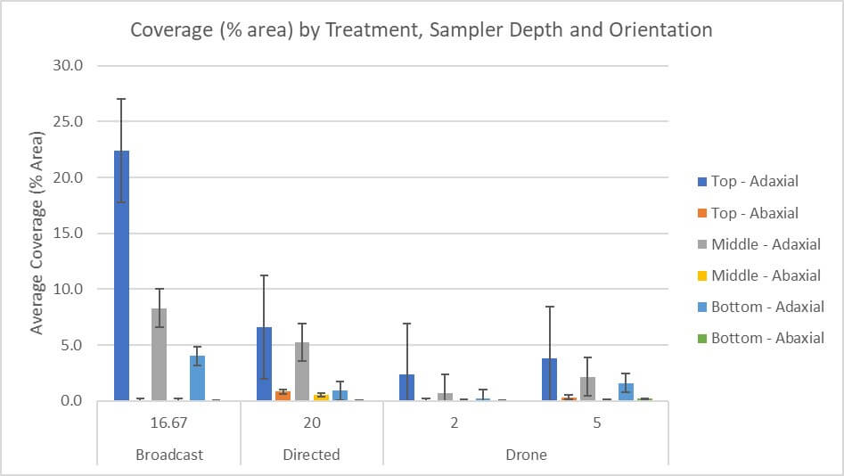
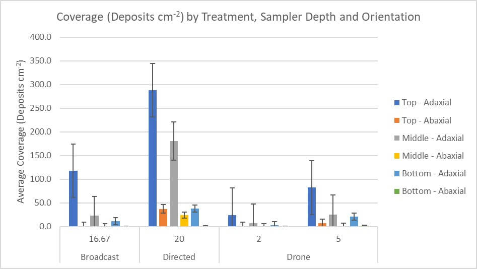
    When we increase resolution to include sampler orientation, we see high standard errors typical of the variability inherent to spray coverage analysis (Figures 6 and 7). The broadcast treatment had the highest average adaxial % area coverage and the second highest average deposit density. The directed treatment had the second highest average adaxial % area coverage and the highest average deposit density but had the highest overall average coverage on the abaxial samplers. RPAS coverage on all samplers was lowest overall and was relative to the volumes applied.

    Figure 6- Coverage (% area) by treatment, sampler depth and orientation.
    Figure 7- Coverage (Deposits cm-2) by treatment, sampler depth and orientation.

    Focusing on RPAS treatments, the orientation of the sampler significantly affected coverage (Tables 19 and 20).

    Sampler OrientationAvg. Coverage (% Area)Sig.Avg. Coverage (Deposits cm-2)Sig.
    Adaxial1.1A11.6A
    Abaxial0.0B0.4B
    Table 19- RPAS (2 gpa) coverage by sampler orientation.
    Sampler OrientationAvg. Coverage (% Area)Sig.Avg. Coverage (Deposits cm-2)Sig.
    Adaxial2.5A47.3A
    Abaxial0.2B7.5B
    Table 20- RPAS (5 gpa) coverage by sampler orientation

    Continuing to focus on the RPAS treatments, the depth of the sampler had a significant effect on overall average coverage at both 2 gpa (Table 21) and 5 gpa (Table 22). Just as with the average % applied rate ac-1 (included here for comparison), the overall average coverage on the top adaxial sampler was significantly higher than the other two depths for % area covered and deposits cm-2.

    Sampler DepthAvg. Coverage
    (% Area)
    Sig.Avg. Coverage
    (Deposits cm-2)
    Sig.Avg.
    % Applied Rate ac-1
    Sig.
    Top1.2A12.8A7.5A
    Middle0.4B3.9B3.8B
    Bottom0.1B1.3B1.7B
    Table 21- Coverage on the top sampler was significantly different than other depths at 2 gpa.
    Sampler DepthAvg. Coverage
    (% Area)
    Sig.Avg. Coverage
    (Deposits cm-2)
    Sig.Avg.
    % Applied Rate ac-1
    Sig.
    Top2.1A48.3A9.2A
    Middle1.1B17.6B5.8B
    Bottom0.9B16.4B2.3B
    Table 22- Coverage on the top sampler was significantly different than other depths at 5 gpa.

    Comparing data from WSP to Mylar Samplers

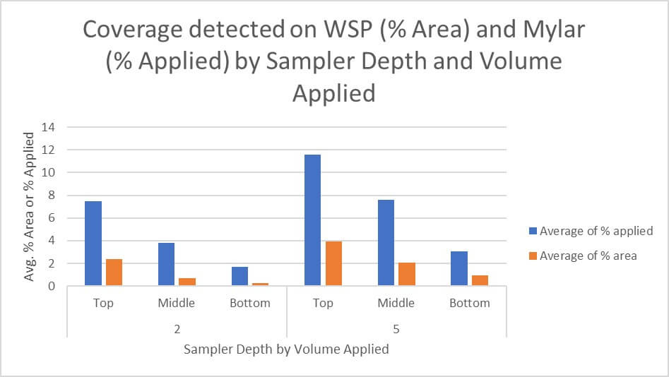
    There was a correlation between the % area coverage detected using WSP and the tracer recovered from the Mylar samplers. Deposit density provides valuable information about the distribution of spray over the target surface but does not always correlate with % area covered, and it is therefore omitted from this comparison. When we plot the average % area covered from the adaxial WSP against the average % applied rate ac-1 from the Mylar samplers, we see the same near-linear pattern of decay with depth (Figure 8).

    Figure 8- Average coverage from adaxial samplers plotted by depth and volume applied show similar coverage patterns.

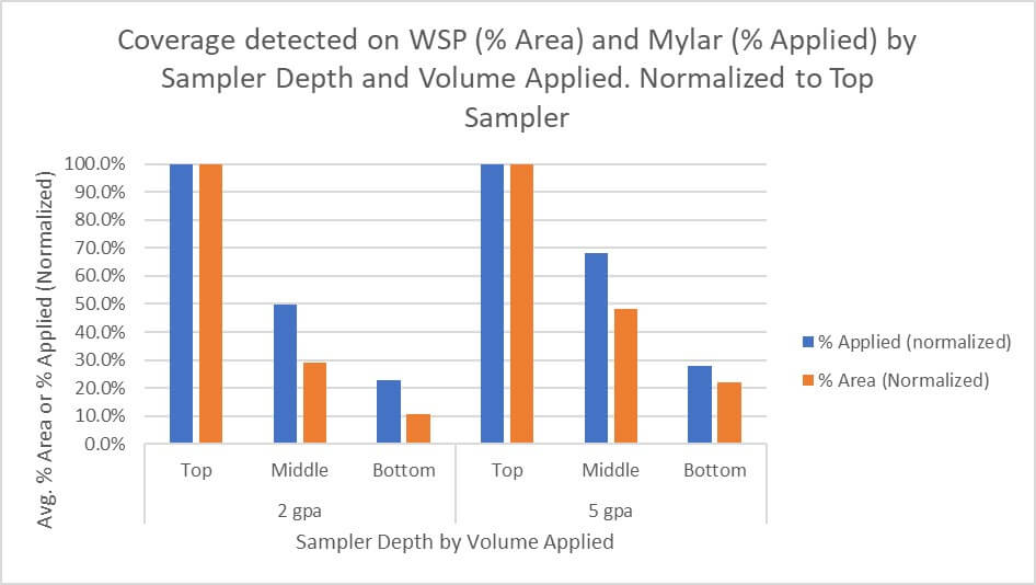
    If we assume each top, adaxial sampler (irrespective of sampler material) represents the highest degree of coverage, we can assign it a value of 100% and index the data to this value. This allows us to visualize and compare the two sampler types directly (Figure 9) and illustrates similar relative coverage, but perhaps a greater rate of decay for the WSP.

    Figure 9- Average coverage from adaxial samplers plotted by depth and volume applied show similar coverage patterns. Normalized to top sampler.

    Net Revenue and Disease Pressure

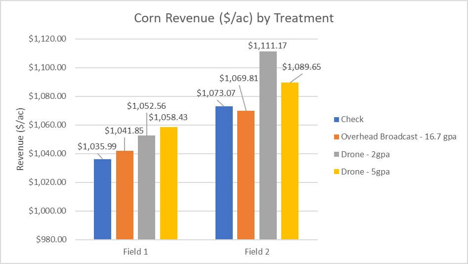
    Crops were harvested at the R4 stage of development. There was no disease pressure detected in any field and no clear impact of application method on net revenue (Figure 10). Results based on the following formula: (CAD $/ac) = (Seed Yield × Corn Sale Price) – Drying Cost. No conclusions regarding efficacy can be drawn from this data.

    Figure 10- Net Revenue (CAD $/ac) by field and treatment.

    Key Observations

    1. Water Sensitive Paper (WSP) measurements of percent area covered (% area) and deposit density (deposits cm-2), and Mylar samplers measuring mass deposit (% applied rate ac-1), revealed similar coverage patterns, making both samplers viable methods for RPAS coverage analysis. These are complimentary methods that reveal different aspects of coverage. When possible, they should be used simultaneously to produce a more complete analysis.
    2. RPAS and conventional overhead broadcast applications produced similar deposition patterns in the corn canopy: A negative linear relationship between coverage and adaxial sampler depth was observed for most treatments (r2=0.997) and abaxial coverage was very low or more often, nonexistent. Further, overall coverage shared a direct relationship with volume for RPAS and conventional overhead broadcast applications.
    3. Directed applications in this study employed a finer spray quality, released laterally from within the canopy. This produced a different coverage pattern than the RPAS and overhead broadcast applications. Per WSP, this treatment resulted in the highest overall deposit density and was the only treatment to produce significant deposition on abaxial surfaces.
    4. For RPAS, spray coverage was significantly reduced by -58% (based on avg. applied rate ac-1), by -59% (based on avg. % covered) and by -74% (based on avg. deposits cm-2) and drift was significantly increased by +73% for the 2 gpa treatments versus the 5 gpa. We attribute this primarily to drone travel speed, which increased from 3.3 m/s at 5 gpa to 7 m/s at 2 gpa. For context, and with certain exceptions, travel speed shares a negative relationship with spray coverage and a direct relationship with drift in airblast and field sprayer applications.
    5. There was a “field effect” where field 2 had lower overall RPAS coverage for both 2 and 5 gpa treatments. Compared to field 1, by -28% for the 2 gpa treatment, and by -41% for 5 gpa. Average drift increased by +76% for 2 gpa and by +77% for 5 gpa. We attribute this to the significantly higher wind conditions in field 2.
    6. Given the lack of disease pressure in the two fields, and the lack of any significant difference in revenue by treatment within each field, efficacy is inconclusive. This study represented only two of eight fields in a larger RPAS efficacy trial where five locations had disease pressure high enough to rate. Preliminary results suggest that Tar Spot control from a 5 gpa drone application may be comparable to that of a 16.7 gpa overhead broadcast application from a field sprayer (data not shown).

    Summary

    Drone and conventional overhead broadcast treatments deposited spray in a similar pattern (a negative linear relationship with canopy depth and very low or no abaxial coverage), irrespective of the method used to analyze coverage. RPAS produced significantly lower coverage than the conventional overhead broadcast treatment, which is attributed primarily to the low volumes employed, per the direct relationship between volume applied and overall coverage (up to some point of diminishing return). High ambient windspeed significantly increased drift in both the 2 and 5 gpa conditions and reduced spray coverage. High travel speeds (required to apply 2 gpa) likely contributed to the significantly increased drift and reduced coverage in that treatment versus 5 gpa. For the use cases explored in this study, low volumes and high travel speeds are not advisable for RPAS, particularly in high wind conditions. Future work separating the travel speed and ambient wind speed variables would clarify their relative influence on RPAS drift and coverage.

    This video presentation is covers the highlights of the study. And disregard the verbal slip-up: we didn’t travel 110 mph.