Category: Coverage

All hort articles about achieving, confirming or correcting for spray coverage.

Rotary-Wing Drone Spray Coverage and Drift in Field Corn

This work was performed with Mark Ledebuhr (Application Insight LLC.), Adrian Rivard (Drone Spray Canada) and Adam Pfeffer (Bayer Crop Science – funding partner). Amy Shi is gratefully acknowledged for her assistance with statistical analysis.

Introduction

In June 2017, Transport Canada cleared the general use of drones. In 2018, Health Canada clarified that the use of Remote Piloted Aircraft Systems (RPAS) for pesticide application is not permitted under the Pest Control Products Act without sufficient data to characterize any associated risk. Currently, there are no liquid pest control products registered for application by drone in Canada.

Stakeholders want to use drones to apply pest control products in Canada. To that end, several research trials have been approved by Health Canada. However, multi-rotor drones represent a unique application technology more akin to air-assisted ground sprayers than manned aircraft. As such, conventional models for drift, exposure and efficacy may not apply. Fundamental questions surrounding the utility of drones must be addressed before efficacy and residue can be considered in any relevant context.

Research and user experience has identified, and is beginning to understand the relative influence of, external factors such as crop morphology, planting architecture, topography, and environmental conditions. Considered with the product mode of action, these factors inform operational settings such as altitude, travel speed, nozzle choice, and application volume to optimize applications. This collective “Use Case” depends on drone design, which is highly variable and rapidly evolving.

Having performed preliminary work characterizing effective swath width, and recognizing its popularity in North America, we used DJI’s Agras T10 in this study. Our objective was to evaluate fungicide efficacy on Northern Corn Leaf Blight, Tar Spot, Grey Spot and Common Rust in field corn, as applied using the T10. Drift and coverage would be characterized to provide context for the efficacy analysis, but also to develop data to inform best practices and possibly regulatory decisions surrounding risk. Aspects of the study would be repeated using conventional ground sprayer technologies to form a basis for comparison.

Objectives

Quantify spray coverage in field corn at three canopy depths, on adaxial and abaxial surfaces, as recovered tracer dye (indexed to % of applied rate ac^-1), area covered (%) and deposit density (deposits cm^-2).
Quantify drift as recovered tracer dye (indexed to % applied rate ac^-1) collected using the horizontal flux method up to eight meters high on the immediate downwind edge of the application.
Evaluate the fungicide efficacy, applied using the T10, at 2 and 5 gpa as compared to a conventional overhead broadcast treatment at 16.7 gpa.

Material and Methods

Design

Trials were conducted between July and August of 2022 in three Ontario corn fields. The locations, the application methods and data collected are detailed in Table 1.

Field	Location	Corn Variety	Application Method	Rate (gpa)	Data Collected
1	Jaffa (42°45’56.6″N 81°02’06.5″W)	DKC45-65RIB	Agras T10	2 and 5	Drift, Coverage, Efficacy
			Overhead Broadcast	16.7	Coverage, Efficacy
2	Fingal (42°42’17.9″N 81°15’15.3″W)	DKC49-09RIB	Agras T10	2 and 5	Drift, Coverage, Efficacy
			Overhead Broadcast	16.7	Efficacy
3	Port Rowan (42°35’53.6″N 80°30’43.2″W)	P0720AM	Directed (Drop hoses)	20	Coverage

Table 1 – Trial sites by application method and data collected

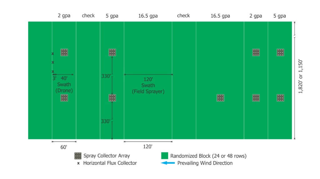
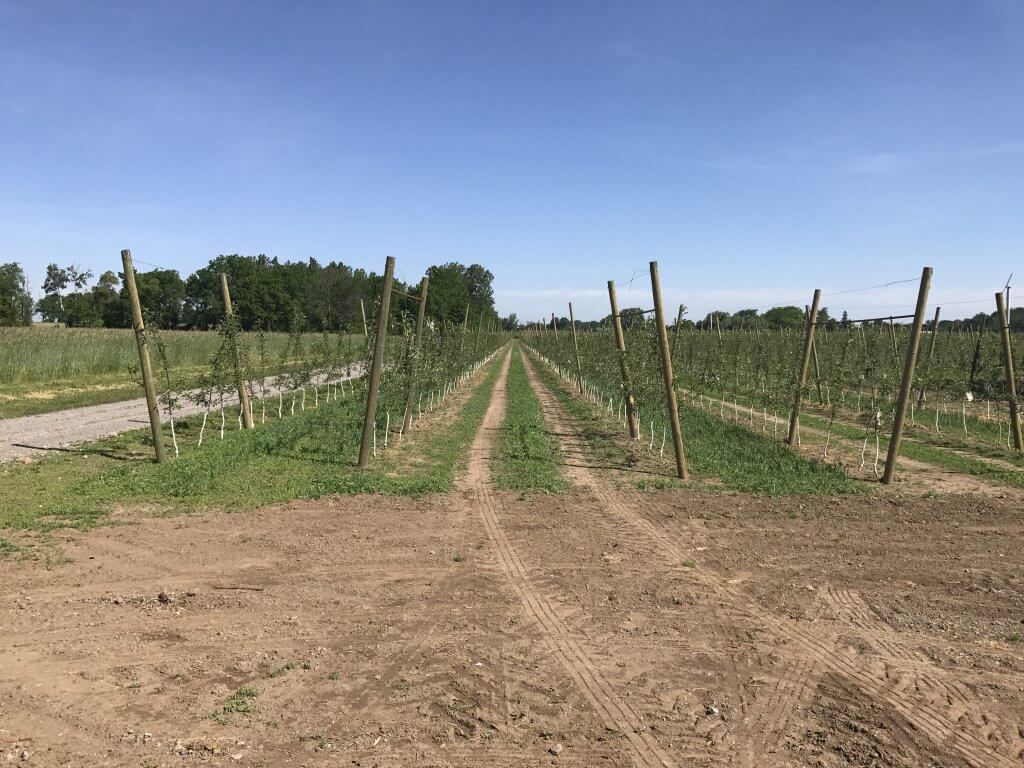
Treatments were arranged in a randomized complete block design (Figure 1). Corn was planted on 30″ centres, with about 6” in-row spacing between stalks. We targeted spray for the R1 stage of development (approx. 8’ high). Fields 1 and 2 each hosted two replicated treatments of 2 gpa, 5 gpa, and 16.7 gpa, as well as two unsprayed checks. In field 1, blocks were 60’ (24 rows) wide by 1,150’ long for the T10, and 120’ (48 rows wide) by 1,150’ long for the broadcast field sprayers. A single, 120’ swath was applied using the field sprayers, and four 10’ (4 row) swaths were required to spray the centre 40’ (16 rows) of corn using the T10. This was based on a 10’ effective swath width determined in previous research. Field 2 had a similar layout but was 1,820’ long.

Figure 1- Sample experimental layout for Field 2. In this example, horizontal flux collectors are positioned 3’ downwind to intercept any off-target drift from the edge of the adjacent 2 gpa treated area.

Coverage Analysis

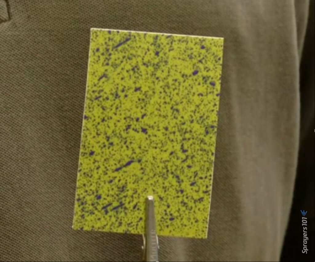
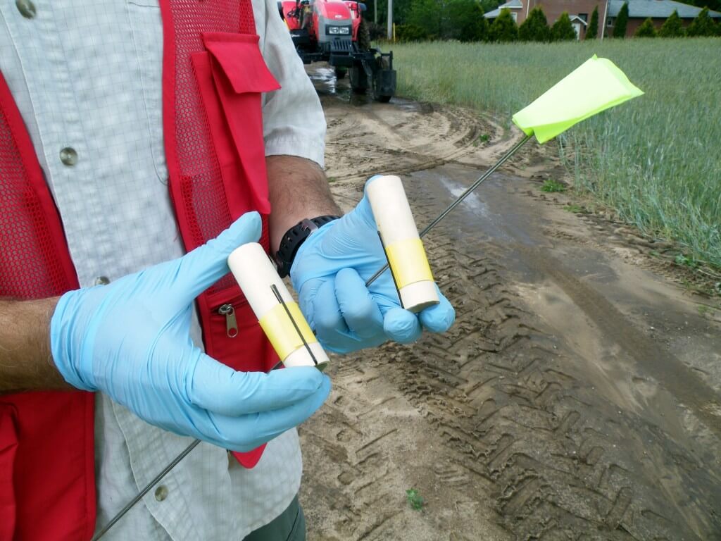
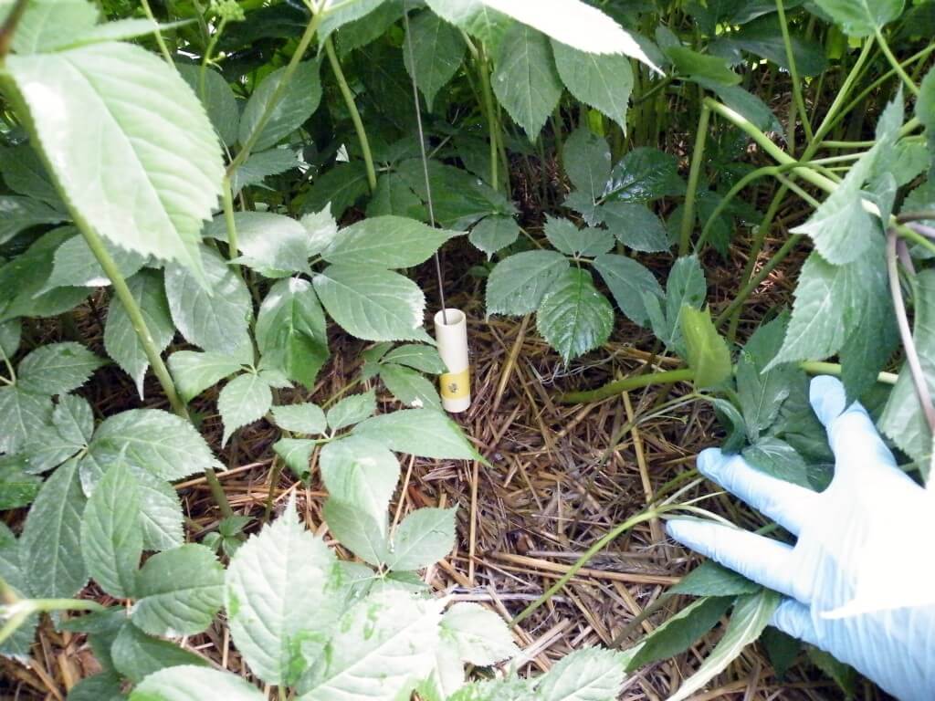
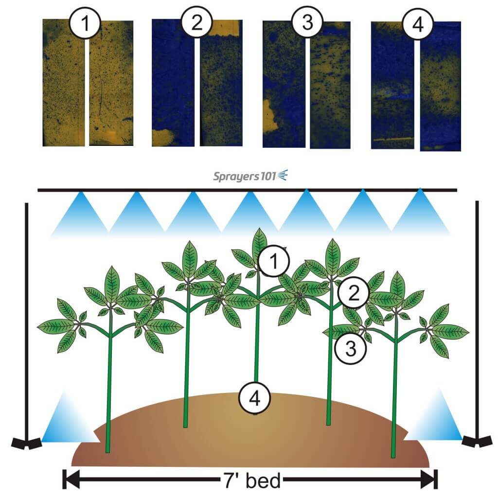
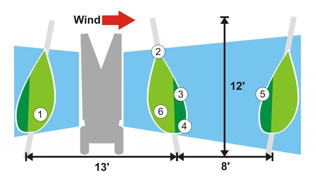
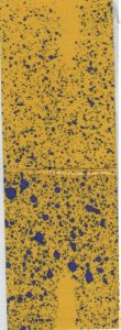
To account for variability, each treatment block was subdivided into two regions, each containing an array of nine spray collectors. Each spray collector (Figure 2) consisted of a vertical, 8’ pole in-row between corn plants. Samplers were attached at three depths to span the silking region: Top: 1.5’-2’ below the tassel. Bottom: 1.5’-2’ from the ground. Middle: halfway between them. Samplers were parallel with the ground to ensure the highest degree of spray interception. On one side, two 1”x3” water sensitive papers (WSP; Innoquest Inc.) were clipped back-to-back with a sensitive side positioned up (adaxial) and facing down (abaxial). The other clip held two 4” square sheets of Mylar in the same orientation. Sampler type was alternated vertically (e.g. Mylar – WSP – Mylar or WSP – Mylar – WSP).

Figure 2- Spray collectors temporarily loaded with WSP and Mylar samplers. These were held above the tassels as they were carried to the collection sites in each block. Three clips were positioned per pole, alternating Mylar and WSP samplers on each side, on two arrays of nine poles, as previously described.

This study used 864 WSP and 864 Mylar samplers for the RPAS treatments, and 162 WSP for the overhead broadcast and directed applications. Following the application, samplers were retrieved as soon as they were dry enough to handle (about 30 minutes) and individually placed into pre-labeled sealable plastic bags, each uniquely coded to the exact position and orientation of the collector.

Operational Use Cases

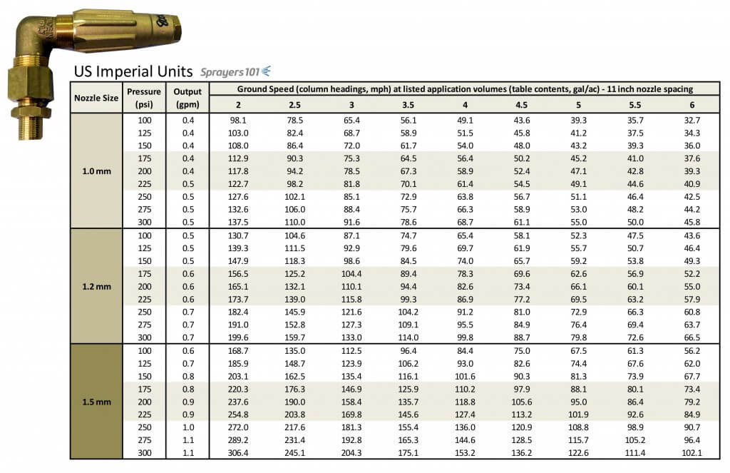
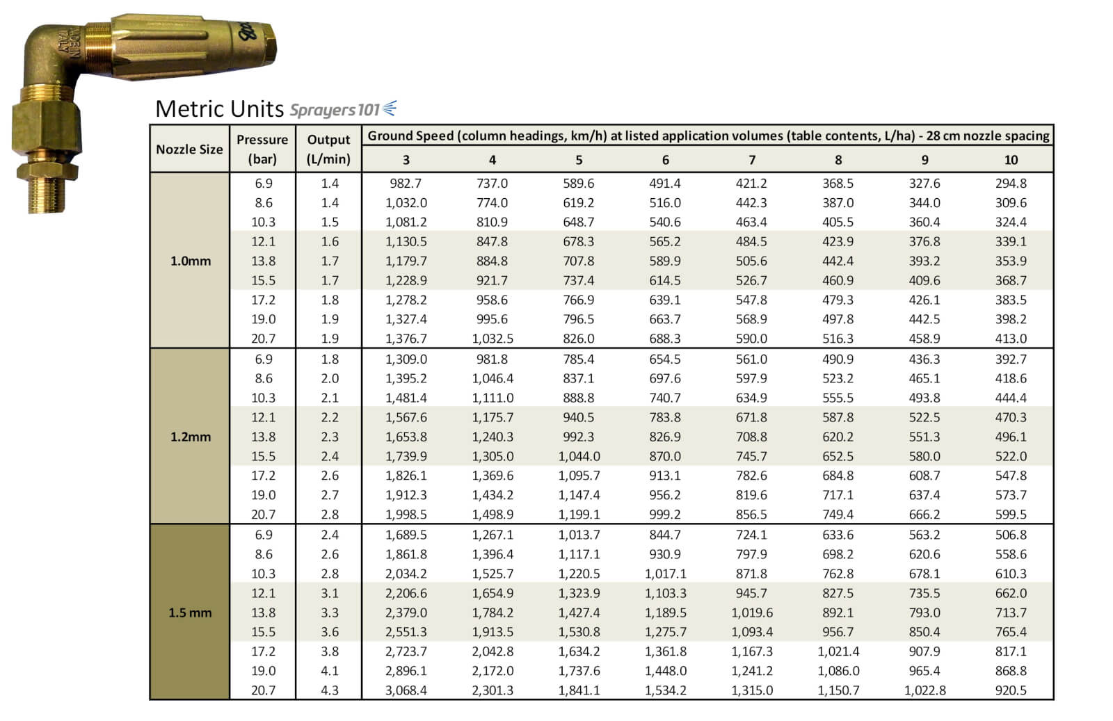
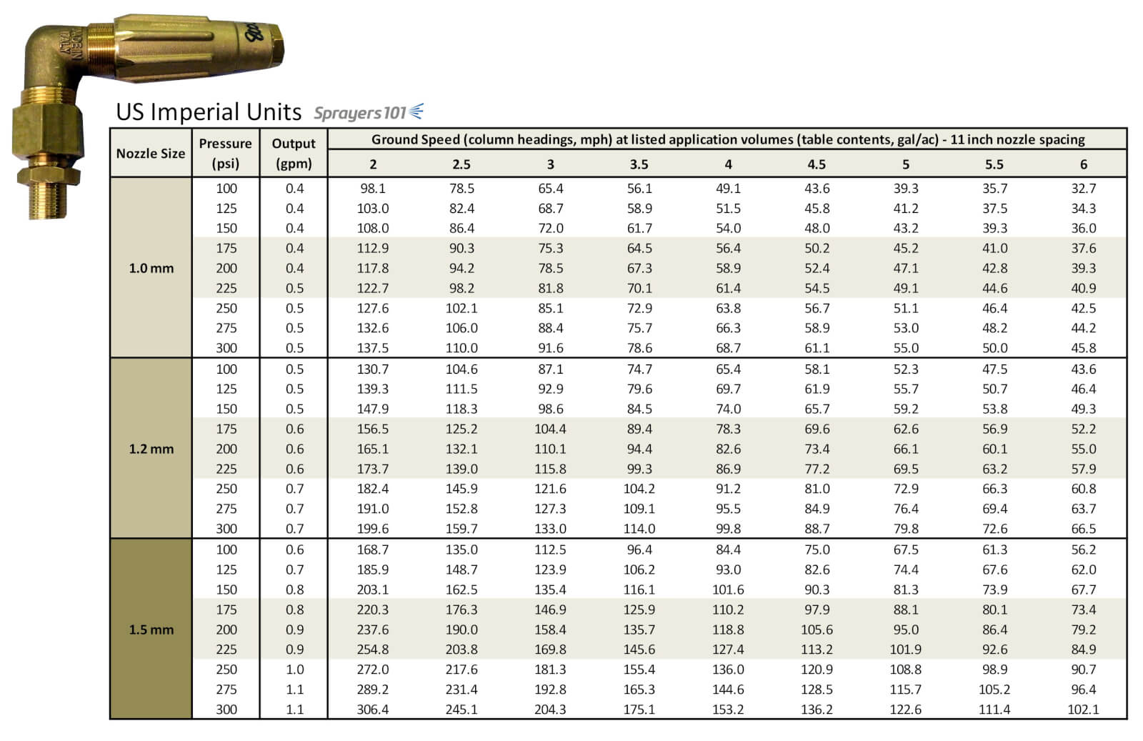
5 gpa: DJI Agras T10 was operated at 3.3 m/s, 2 m above tassels. TeeJet 11002 AIXR nozzles equipped with 50 mesh filters were operated at 70 psi.
2 gpa: DJI Agras T10 was operated at 7.0 m/s, 2 m above tassels. TeeJet 11002 AIXR nozzles equipped with 50 mesh filters were operated at 45 psi.
16.7 gpa: Overhead broadcast condition. Field 1 ran a John Deere 4038R operated at approx. 10 mph with TeeJet XR11006 nozzles on 20” spacing. Pulse width modulation (ExactApply) was engaged. Field 2 ran a New Holland 345 front-mounted boom sprayer with TeeJet XR11006 nozzles on 20” spacing.
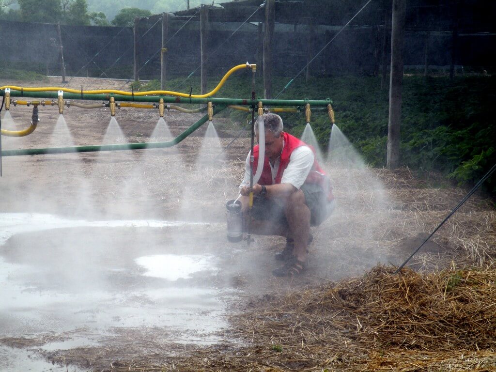
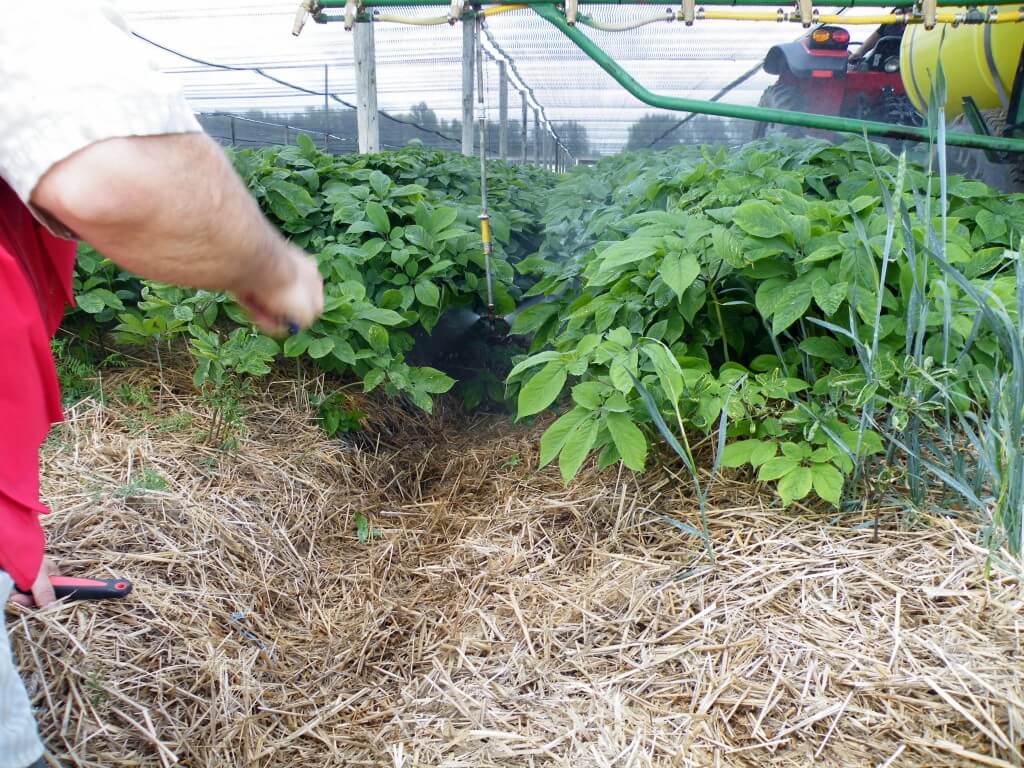
20 gpa: Directed condition. John Deere R4038 operated at approx. 4.5 mph with Beluga drop hoses suspended on 30” centres to correspond with alley spacing. Two nozzle bodies were positioned 15″ apart equipped with Greenleaf Spray Max 110015 nozzles to span the silking area.

Drift Analysis

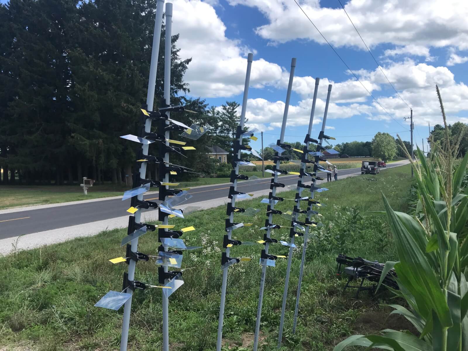
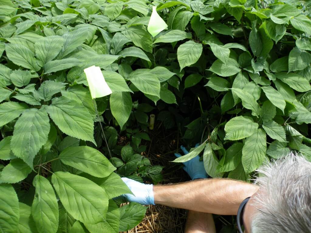
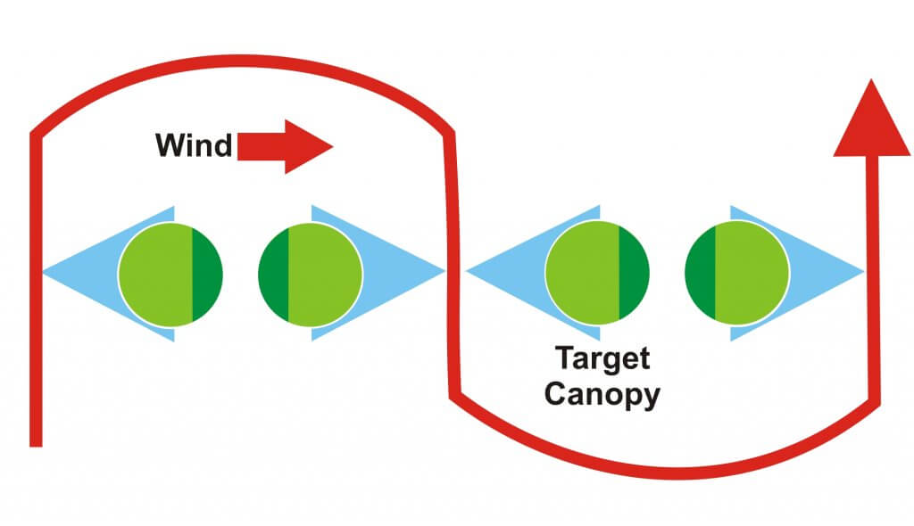
Three free-standing 26’ (8 m) horizontal flux collectors were positioned in the corn field approximately 3’, or 1.5 rows from the downwind edge of the spray plot downwind of the area treated by drone (Figure 3). The sampling poles were positioned about 30’ apart parallel to the treatment block. Sterilized, 1.8 mm braided polyethylene collector line was run up the poles on pulleys just prior to application. Following applications, the line was collected in 1 m lengths into sealed bags.

The assumption was that by placing the horizontal flux samplers as close to the “zero” downwind edge position as possible, nearly the entire off-swath movement of drift would be captured. A compromise of placing the samplers in the middle of the first row past the downwind swath edge was made due to the scale of the sample and the relative low swath precision of the drone. Placing the samplers closer to the zero downwind line was deemed to be too high a risk of inadvertently sampling in-swath.

Figure 3- Moving horizontal flux poles into the field prior to positioning them for trials. String collectors were run up the poles just before spray application and retrieved immediately afterwards.

Spray Solution (Formulated Product plus Tracer)

Fungicide was applied at field rates (8 oz/ac or 586 mL/ha). The field sprayer applied this at 16.7 gpa. The drone applied it at 2 or 5 gpa but also included tracer solution at 0.2% (20 ml/10L solution) vol./vol. of a 20% mass/mass solution of PTSA in dH₂O. PTSA residue data assumes 100% recovery and 0% degradation of the tracer. Tests of PTSA with fungicide prior to the study showed no physical antagonism and >98% tracer recovery. Prior testing of PTSA showed an acceptable 1-2% solar degradation in the timeframe required to collect samplers. Tank samples were drawn from the drone at the beginning and end of each trial and used to confirm tank concentration and to establish fluorescence curves.

Weather Conditions

Weather data was collected using a Kestrel 3550AG weather meter (Kestrel Instruments) in a vane mount positioned 1 m above the tassel (approximately 1 m below drone altitude). Data was logged every 5 seconds. Issues with data loss required us to supplement local data with Field Level Weather Summary data (Table 2).

Date (2022)	Field	Vol. (gpa)	Avg. Temp. (°C)	Avg. Windspeed (km/h)	Start Time	Duration (min.)
Jul 25	1	5*	22.3	6.2	13:00	35
Jul 25	1	5	21.4	7.5	18:45	35
Jul 26	1	16.7	18.8	5.4	10:00	45
Jul 26	1	2	23.9	7.7	15:30	25
Jul 29	2	5**	n/a	16.4	11:00	35
Jul 29	2	2***	23.6	21.0	14:00	25
Aug 12	3	20****	25.4	6.3	13:30	15

Table 2- Date, location, and weather conditions for each treatment
*Trial pass over spray collectors only – no horizontal flux collectors employed.
**All bottom-level water sensitive paper samplers spoiled by high humidity. Wind changeable and horizontal flux poles moved 2x before application to orient downwind.
***Noted flocculation in tank samples likely from rainfastness adjuvant. Did not affect analysis.
****Coverage data from a single array of nine spray collectors with water sensitive paper samplers.

Results

Statistics

The % applied rate ac^-1, % area covered, and deposits cm^-2 were subjected to analysis of variance using SAS^® OnDemand for Academics PROC GLM. When a significant treatment effect was found, means were compared using Tukey’s honest significant difference test (HSD) at p=0.05.

Data Collation

Each spray collector was a vertical structure that supported Mylar samplers at three depths. Each depth held two samplers oriented abaxially or adaxially, in parallel with the ground. When discussing the amount of PTSA recovered by sampler depth or by sampler orientation, the % applied rate ac^-1 of each of the nine related samplers were averaged within each array (n=2 arrays per block times two replicates equal n=4 per treatment).

When considered from above, the six Mylar samplers are vertical cross-sections of the same area of ground. Therefore, the % applied rate ac^_-1from each sampler was added to represent the total mass of tracer intercepted per collector. When these nine sub-samples are averaged, we arrive at the average % applied rate ac^-1 per array.

Similarly, the % applied rate ac^-1 from each 1 m length of string on a horizontal flux collector could be averaged across collectors by relative position to explore drift by height (n=3 poles per block times two replicates equal n=6 per treatment). Alternately, the total PTSA recovered per pole could be calculated (n=3 poles per block times two replicates equal n=6 per treatment). This interpretation allowed us to perform a mass balance accounting of residue in-canopy and as drift compared to the known applied rate ac^-1.

It was not possible to collate the data in this fashion for the WSP because it was not possible to index % area or deposits cm^-2 on a 1”x3” area to a theoretical maximum. Therefore, we averaged the nine samplers within an array relative to their position and orientation (n=2 arrays per block times two replicates equal n=4 per treatment) or averaged the six samplers per collector prior to averaging all collectors in an array (n=2 arrays per block times two replicates equal n=4 per treatment).

RPAS Coverage – Mylar Samplers

There is a negative linear relationship (r²=0.997) between the depth of the sampler and the average % applied rate ac^-1 (Table 3). The deeper the sampler, the less tracer recovered. The sum of the average % applied rate ac^-1at each depth was 17.7% of known rate applied rate ac^-1.

Sampler Depth	Avg. % Applied Rate ac^-1	Significance
Top	9.6	A
Middle	5.7	B
Bottom	2.4	C
Total:	*17.7*	–

Table 3- The depth of the sampler had a significant effect on the overall average amount of PTSA recovered.

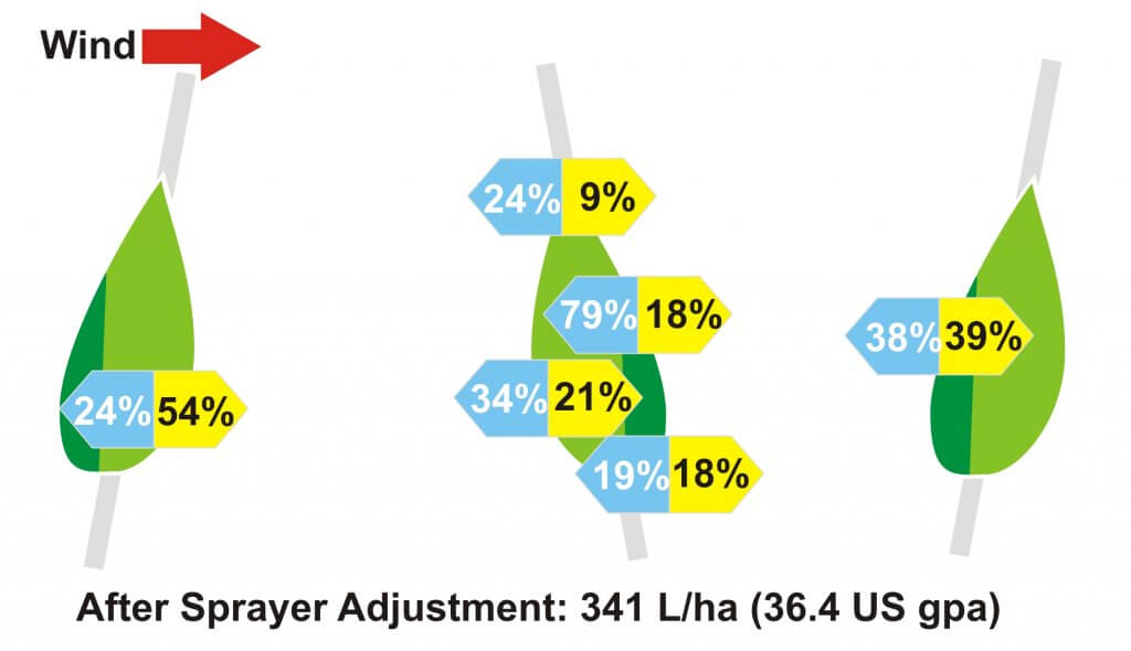
The orientation of the sampler significantly affected the overall average amount of tracer recovered (Table 4). The abaxial surfaces intercepted an average 11.1 % applied rate ac^-1 less (a 97% difference) than adaxial surfaces. Note: When Mylar was retrieved a few had physically shifted, potentially exposing the back side of abaxial collectors to primary deposition from above. Therefore, it is assumed that the actual deposit is lower than reported here.

Sampler Orientation	Avg. % Applied Rate ac^-1	Significance
Adaxial	11.4	A
Abaxial	0.3	B

Table 4- The orientation of the sampler had a significant effect on the overall average amount of PTSA recovered.

When we separate the data to focus on the volume applied, we see volume had a significant impact on the amount of tracer recovered (Table 5). The average % applied rate ac^-1 was 2.1% less (a 58% difference) in the 2 gpa condition compared to the 5 gpa condition.

Field	Avg. % Applied Rate ac^-1	Significance
1	7.1	A
2	4.6	B

Table 5- The field location had a significant impact on the average amount of PTSA recovered.

When we isolate the volume applied by field, the 2 gpa treatment resulted in less coverage in field 2 (average 1.4 % applied rate ac^-1 or 28% less) and significantly for the 5 gpa treatment (average 3.6 % applied rate ac^-1 or 41% less: Table 6).

Date	Field	Volume (gpa)	Avg. % Applied Rate ac^-1	Significance
Jul 25	1	5	9.2	A
Jul 26	1	2	5.0	B
Jul 29	2	5	5.6	C
Jul 29	2	2	3.6	B

Table 6- The average amount of PTSA recovered by date and location show lower overall recovery in Field 2.

When sampler depth is included in the field analysis (Table 7), we see similar deposition patterns; a negative linear relationship between coverage and canopy depth in all treatments save the 5 gpa treatment in field 2. Closer inspection confirms a reduction in coverage for the 2 gpa condition in field 2 versus field 1, and a significant reduction for the 5 gpa condition in field 2 versus field 1.

Sampler Depth	Field 1 – Jul 25: 5 gpa. Avg. % Applied Rate ac^-1 (Sig.)	Field 1 – Jul 26: 2 gpa. Avg. % Applied Rate ac^-1 (Sig.)	Field 2 – Jul 25: 5 gpa. Avg. % Applied Rate ac^-1 (Sig.)	Field 2 – Jul 29: 2 gpa. Avg. % Applied Rate ac^-1 (Sig.)
Top	15.2 (A)	8.3 (A)	8.0 (A)	6.7 (A)
Middle	9.1 (B)	4.7 (B)	6.1 (AB)	2.9 (B)
Bottom	3.5 (B)	1.9 (C)	2.6 (B)	1.5 (B)
*Total:*	*27.8*	*14.9*	*16.7*	*11.1*

Table 7- The average residue recovered by date, location and sampler depth is significantly less in the 5 gpa condition in field 2 and does not distribute linearly by sampler depth.

RPAS Drift – Horizontal Flux

Overall, the volume applied had a significant impact on drift, where the 2 gpa treatment resulted in an average increase of 1.6 % applied rate ac^-1 (44% difference: Table 8) versus the 5 gpa treatment.

Volume Applied (gpa)	Avg. % Applied Rate ac^-1	Significance
2	3.6	A
5	2.0	B

Table 8- The volume applied had a significant impact on the amount of the PTSA recovered.

As with the Mylar samplers, there was a “field effect” where the field had a statistically significant impact on the amount of tracer recovered (Table 9). However, unlike the Mylar samplers in the crop, more tracer was recovered in field 2 (average increase of 3.2 applied rate ac^-1 or a 67% difference) than in field 1.

Field	Avg. % Applied Rate ac^-1	Significance
1	1.4	A
2	4.2	B

Table 9- The field location had a significant impact on the amount of PTSA recovered.

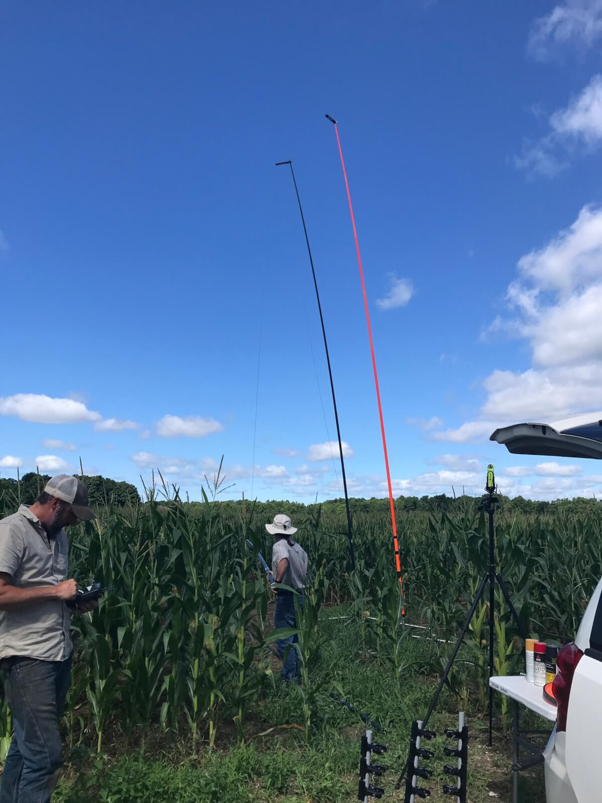
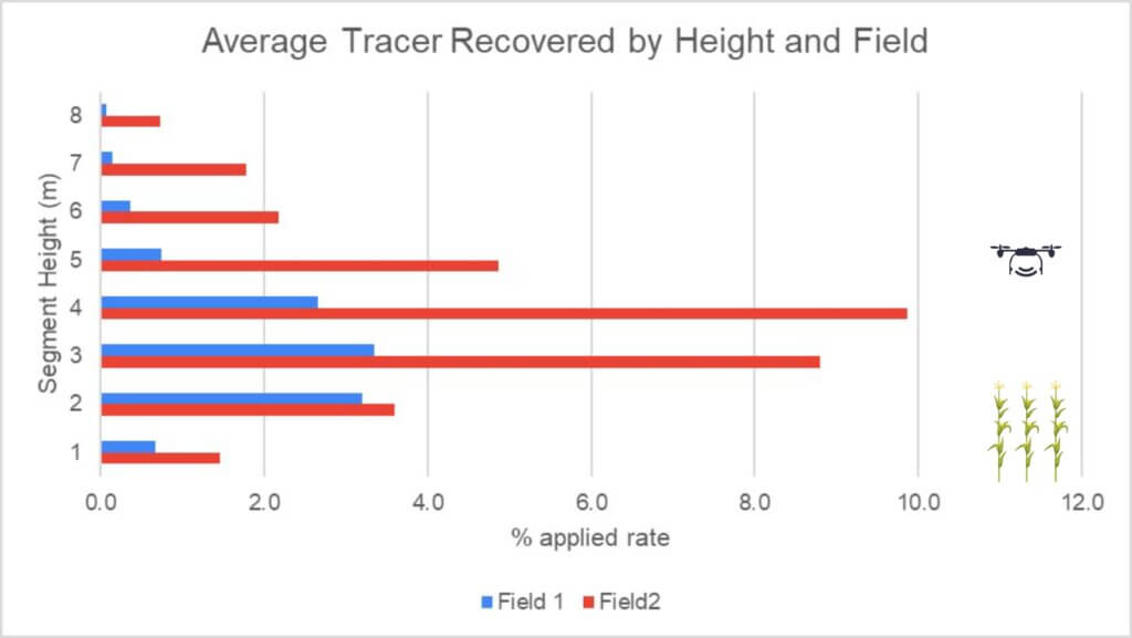
The pattern of deposition by height was similar across all treatments. For context, note that the first 2.5-3 m of string were within the corn canopy and drone altitude was approximately 5 m off the ground (2 m over the tassels) per Figure 4 and 5. The differences were only statistically significant in field 2 (Table 10) where an average 33% applied rate ac^-1 was intercepted compared to 11% in field 1.

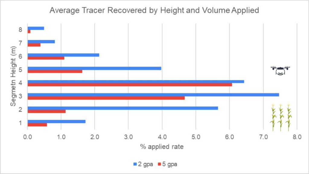
Figure 4- Average PTSA recovered (% applied rate ac^-1) by height and field.

Figure 5- Average PTSA recovered (% applied rate ac^-1) by height and volume applied.

Height (1m segment in m from ground)	Field 1: Avg. % Applied Rate ac^-1	Sig.	Field 2: Avg. % Applied Rate ac^-1	Sig.
8	0.7	A	1.5	C
7	3.2	A	3.6	BC
6	3.3	A	8.8	A
5	2.7	A	9.9	A
4	0.7	A	4.9	AB
3	0.4	A	2.2	BC
2	0.1	A	1.8	C
1	0.1	A	0.7	C
*Total:*	*11.2*	–	*33.3*	–

Table 10- The average amount of PTSA recovered by height for field 1 and field 2.

The volume applied had a significant effect on the total PTSA tracer detected in both fields, with an average 4.4% applied rate ac^-1 more (a 59% difference) recovered in the 2 gpa treatment (Table 11 and Figure 5). Separated by fields, the 5 gpa treatment had an average 1.4% % applied rate ac-1 more (a 77% difference) in field 2 and the 2 gpa treatment had an average 2.8% % applied rate ac^-1 more (a 76% difference) in field 2.

Volume Applied (gpa)	Field 1: Avg. % Applied Rate ac^-1	Sig.	Field 2: Avg. % Applied Rate ac^-1	Sig.
2	2.2	A	5.0	A
5	0.7	B	2.1	B

Table 11- The volume applied had a significant impact on the amount of PTSA recovered.

Mass Balance Accounting

It is never possible to entirely “close mass” in spray studies because there are other surfaces (e.g. leaves) within the vertical profile that intercept spray, as well as off-swath deposition and the ground itself (not measured in this study). Nevertheless, the exercise does allow us to estimate and compare how much spray was captured and how much remains unaccounted for (Table 12). We see that the 2 gpa treatment in field 1 had the highest unaccounted-for fraction, and on average we were able to account for an average 53% of the applied rate ac^-1 in this study.

Field (Volume in gpa)	Coverage: Avg % Applied Rate ac^-1 (A)	Drift: Avg % Applied Rate ac^-1 (B)	Total % Detected (A+B)	Unaccounted Fraction [100-(A+B)]
1 (5)	51	5	56	44
1 (2)	26.5	17	43.5	56.5
2 (5)	30	24	54	46
2 (5)	19.5	40	59.5	40.5

Table 12- Closing mass using % PTSA detected on in-canopy samplers and on drift collectors.

RPAS and ground rig coverage – Water Sensitive Paper

The depth of the sampler had a significant effect on the overall average % area covered at all depths (Table 13). However, there was no significant difference at the two lower depths for deposit density (Table 14). In both cases, the negative linear relationship between coverage and sampler depth corresponds closely to the PTSA recovered on the Mylar samplers (see Table 3).

Sampler Depth	Avg. Coverage (% Area)	Significance
Top	2.80	A
Middle	1.28	B
Bottom	0.62	C

Table 13- Overall average % coverage by sampler depth.

Sampler Depth	Avg. Coverage (Deposits cm^-2)	Significance
Top	44.5	A
Middle	17.9	B
Bottom	7.2	C

Table 14- Overall average deposit density by sampler depth.

The sampler orientation had a significant effect on both overall average % area covered (Table 15) and deposits cm^‑2 (Table 16).

Sampler Orientation	Avg. Coverage (% Area)	Significance
Adaxial	3.03	A
Abaxial	0.12	B

Table 15- The orientation of the sampler had a significant effect on the average % area covered.

Sampler Orientation	Avg. Coverage (Deposits cm^-2)	Significance
Adaxial	43.5	A
Abaxial	3.1	B

Table 16- The orientation of the sampler had a significant effect on the average deposit density.

The treatment had a significant effect on the overall % coverage (Table 17) with the overhead broadcast condition covering an average 3.31% more sampler surface (a 60% difference) compared to the next highest treatment value. The directed application delivered a significantly higher 67 deposits cm^-2 (a 72% difference) compared to the next highest treatment value (Table 18).

Treatment (gpa)	Avg. Coverage (% Area)	Significance
Broadcast (16.7)	5.91	A
Directed (20)	2.32	B
Drone (5)	1.34	BC
Drone (2)	0.55	C

Table 17- Overall average % coverage by treatment.

Treatment (gpa)	Avg. Coverage (Deposits cm^-2)	Significance
Broadcast (16.7)	92.6	A
Directed (20)	25.8	B
Drone (5)	22.9	B
Drone (2)	5.9	B

Table 18- Overall average deposit density by treatment.

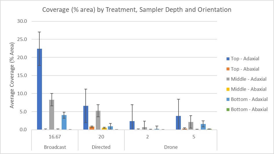
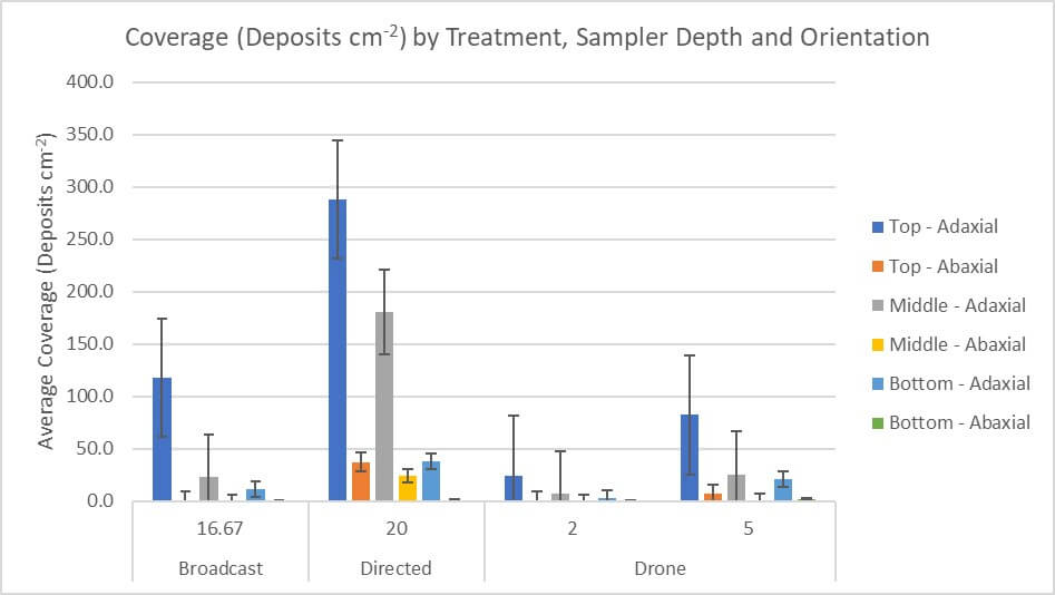
When we increase resolution to include sampler orientation, we see high standard errors typical of the variability inherent to spray coverage analysis (Figures 6 and 7). The broadcast treatment had the highest average adaxial % area coverage and the second highest average deposit density. The directed treatment had the second highest average adaxial % area coverage and the highest average deposit density but had the highest overall average coverage on the abaxial samplers. RPAS coverage on all samplers was lowest overall and was relative to the volumes applied.

Figure 6- Coverage (% area) by treatment, sampler depth and orientation.

Figure 7- Coverage (Deposits cm^-2) by treatment, sampler depth and orientation.

Focusing on RPAS treatments, the orientation of the sampler significantly affected coverage (Tables 19 and 20).

Sampler Orientation	Avg. Coverage (% Area)	Sig.	Avg. Coverage (Deposits cm^-2)	Sig.
Adaxial	1.1	A	11.6	A
Abaxial	0.0	B	0.4	B

Table 19- RPAS (2 gpa) coverage by sampler orientation.

Sampler Orientation	Avg. Coverage (% Area)	Sig.	Avg. Coverage (Deposits cm^-2)	Sig.
Adaxial	2.5	A	47.3	A
Abaxial	0.2	B	7.5	B

Table 20- RPAS (5 gpa) coverage by sampler orientation

Continuing to focus on the RPAS treatments, the depth of the sampler had a significant effect on overall average coverage at both 2 gpa (Table 21) and 5 gpa (Table 22). Just as with the average % applied rate ac^-1 (included here for comparison), the overall average coverage on the top adaxial sampler was significantly higher than the other two depths for % area covered and deposits cm^-2.

Sampler Depth	Avg. Coverage (% Area)	Sig.	Avg. Coverage (Deposits cm^-2)	Sig.	Avg. % Applied Rate ac^-1	Sig.
Top	1.2	A	12.8	A	7.5	A
Middle	0.4	B	3.9	B	3.8	B
Bottom	0.1	B	1.3	B	1.7	B

Table 21- Coverage on the top sampler was significantly different than other depths at 2 gpa.

Sampler Depth	Avg. Coverage (% Area)	Sig.	Avg. Coverage (Deposits cm^-2)	Sig.	Avg. % Applied Rate ac^-1	Sig.
Top	2.1	A	48.3	A	9.2	A
Middle	1.1	B	17.6	B	5.8	B
Bottom	0.9	B	16.4	B	2.3	B

Table 22- Coverage on the top sampler was significantly different than other depths at 5 gpa.

Comparing data from WSP to Mylar Samplers

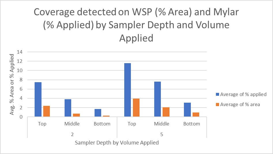
There was a correlation between the % area coverage detected using WSP and the tracer recovered from the Mylar samplers. Deposit density provides valuable information about the distribution of spray over the target surface but does not always correlate with % area covered, and it is therefore omitted from this comparison. When we plot the average % area covered from the adaxial WSP against the average % applied rate ac^-1 from the Mylar samplers, we see the same near-linear pattern of decay with depth (Figure 8).

Figure 8- Average coverage from adaxial samplers plotted by depth and volume applied show similar coverage patterns.

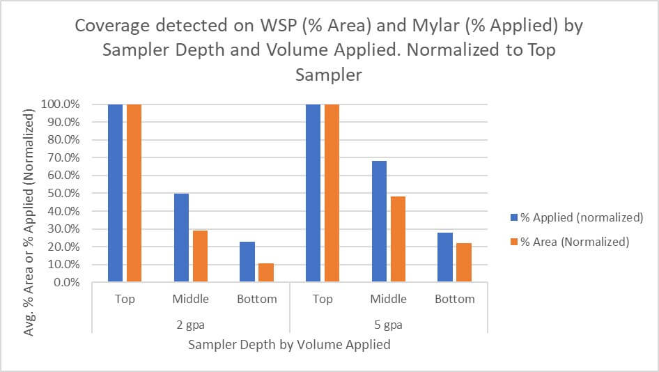
If we assume each top, adaxial sampler (irrespective of sampler material) represents the highest degree of coverage, we can assign it a value of 100% and index the data to this value. This allows us to visualize and compare the two sampler types directly (Figure 9) and illustrates similar relative coverage, but perhaps a greater rate of decay for the WSP.

Figure 9- Average coverage from adaxial samplers plotted by depth and volume applied show similar coverage patterns. Normalized to top sampler.

Net Revenue and Disease Pressure

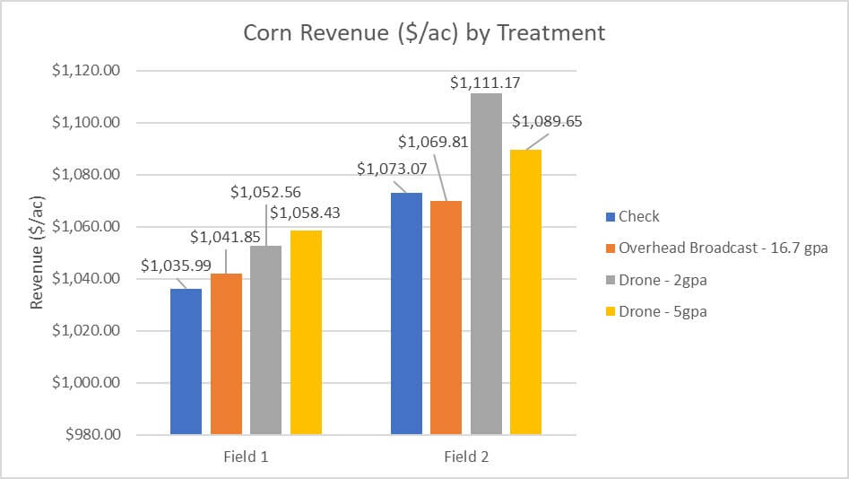
Crops were harvested at the R4 stage of development. There was no disease pressure detected in any field and no clear impact of application method on net revenue (Figure 10). Results based on the following formula: (CAD $/ac) = (Seed Yield × Corn Sale Price) – Drying Cost. No conclusions regarding efficacy can be drawn from this data.

Figure 10- Net Revenue (CAD $/ac) by field and treatment.

Key Observations

Water Sensitive Paper (WSP) measurements of percent area covered (% area) and deposit density (deposits cm^-2), and Mylar samplers measuring mass deposit (% applied rate ac^-1), revealed similar coverage patterns, making both samplers viable methods for RPAS coverage analysis. These are complimentary methods that reveal different aspects of coverage. When possible, they should be used simultaneously to produce a more complete analysis.
RPAS and conventional overhead broadcast applications produced similar deposition patterns in the corn canopy: A negative linear relationship between coverage and adaxial sampler depth was observed for most treatments (r²=0.997) and abaxial coverage was very low or more often, nonexistent. Further, overall coverage shared a direct relationship with volume for RPAS and conventional overhead broadcast applications.
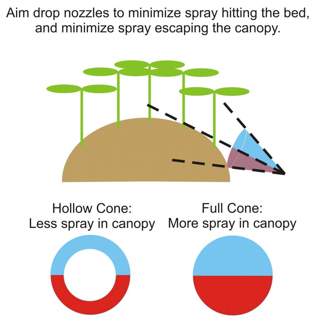
Directed applications in this study employed a finer spray quality, released laterally from within the canopy. This produced a different coverage pattern than the RPAS and overhead broadcast applications. Per WSP, this treatment resulted in the highest overall deposit density and was the only treatment to produce significant deposition on abaxial surfaces.
For RPAS, spray coverage was significantly reduced by -58% (based on avg. applied rate ac^-1), by -59% (based on avg. % covered) and by -74% (based on avg. deposits cm^-2) and drift was significantly increased by +73% for the 2 gpa treatments versus the 5 gpa. We attribute this primarily to drone travel speed, which increased from 3.3 m/s at 5 gpa to 7 m/s at 2 gpa. For context, and with certain exceptions, travel speed shares a negative relationship with spray coverage and a direct relationship with drift in airblast and field sprayer applications.
There was a “field effect” where field 2 had lower overall RPAS coverage for both 2 and 5 gpa treatments. Compared to field 1, by -28% for the 2 gpa treatment, and by -41% for 5 gpa. Average drift increased by +76% for 2 gpa and by +77% for 5 gpa. We attribute this to the significantly higher wind conditions in field 2.
Given the lack of disease pressure in the two fields, and the lack of any significant difference in revenue by treatment within each field, efficacy is inconclusive. This study represented only two of eight fields in a larger RPAS efficacy trial where five locations had disease pressure high enough to rate. Preliminary results suggest that Tar Spot control from a 5 gpa drone application may be comparable to that of a 16.7 gpa overhead broadcast application from a field sprayer (data not shown).

Summary

Drone and conventional overhead broadcast treatments deposited spray in a similar pattern (a negative linear relationship with canopy depth and very low or no abaxial coverage), irrespective of the method used to analyze coverage. RPAS produced significantly lower coverage than the conventional overhead broadcast treatment, which is attributed primarily to the low volumes employed, per the direct relationship between volume applied and overall coverage (up to some point of diminishing return). High ambient windspeed significantly increased drift in both the 2 and 5 gpa conditions and reduced spray coverage. High travel speeds (required to apply 2 gpa) likely contributed to the significantly increased drift and reduced coverage in that treatment versus 5 gpa. For the use cases explored in this study, low volumes and high travel speeds are not advisable for RPAS, particularly in high wind conditions. Future work separating the travel speed and ambient wind speed variables would clarify their relative influence on RPAS drift and coverage.

This video presentation is covers the highlights of the study. And disregard the verbal slip-up: we didn’t travel 110 mph.

July 20, 2023

Airblast Sprayers for Small Operations
Did you come here looking for advice on which sprayer is best for your small operation? Are you looking to ditch the backpack mist blower? Do you want to avoid repeatedly mounting and dismounting a 3-pt hitch sprayer from your only tractor? Are you concerned you’ll have to sell an organ to be able to afford one? We hear you, and we’ll try to help. Let’s set the stage with a few facts.
Airblast sprayers stay in service for a long time; more than twenty five years is not unheard of. The majority of them are the generalist, PTO-driven low profile radial design with capacities ranging 150 to 1,200 gallons. Typical fan diameters are around 30″ and can produce >40,000 m³/h of air, making them a good fit for most pomme, citrus and tender fruit canopies. These sprayers come with a horsepower price tag of perhaps 45 hp or more. Many of these sprayers eventually enter the used sprayer market, making them an affordable option for small acreage specialty operations. But, affordability should not be the sole motivation when choosing a sprayer.
Ontario, c.1980 and probably still out there spraying somewhere!
The key to optimizing sprayer performance is to match the air settings to the the canopy you’re trying to spray. You can start reading about the process here. In the case of small and medium-sized canopies like vine, cane and bush crops, the fleet of gently-used sprayers we just described tend to produce too much air. There are options to improve the fit, like driving faster to reduce dwell time, or perhaps the operator can employ the Gear-up Throttle-down method. But, the best plan is to employ a smaller sprayer, which produces a more appropriate air volume, has a smaller profile, delivers better fuel efficiency and won’t break the bank.
So, where are these sprayers? Unfortunately there aren’t many, and options are especially limited if you don’t own a tractor to power them.
The budget-conscious grower may be tempted to buy a sprayer that does not have air-assist. We do not recommend this. Air is a critical component for spraying canopies consistently and efficiently. Caveat Emptor!
We encountered a good solution in June, 2014, when we were invited to Durocher Farm in New Hampshire to see their new airblast sprayer. In years previous, spotted-wing drosophila (SWD) was a significant pest in this two acre, high bush blueberry planting. They claimed that since buying their new sprayer they no longer had any trouble with SWD. That’s quite an endorsement!
The Carrarospray ATVM (200 L option pictured)
I’m not sure what I expected, but I was captivated by this miniature orchard sprayer. The toy-like size carried a zero-intimidation factor and I immediately wanted to start using it. Italian-made, Carrarospray’s hobby line is designed to be pulled behind vehicles without PTO. The ATVM is available in capacities from 120-400 L. The one I saw had a 400 L capacity, adjustable air deflectors, a fan speed gear box, and it was powered by a quiet and efficient pull-start Briggs & Stratton four-stroke engine. It even had a trash guard, a kick-stand and a clean water tank for hand washing. That’s a lot of features.
Thanks to Kitt Plummer (Durocher Farm), Penn State, Univ. New Hampshire and Chazzbo Media for filming these 2014 videos:
The sprayer was pulled (in this case) by a mower, so the grower not only sprayed, but mowed his alleys at the same time. It fit beautifully between the bushes, so the potential for physical damage to the berries was minimized. The air speed and volume was enough to displace the air in the blueberry canopy and replace it with spray-laden air with minimal blow-through. Combined with an appropriate spray volume and distribution over the boom, we found that the coverage it provided was excellent.
Coverage from the top-centre of the bush.
Since seeing this sprayer, we have had reports that importing it to Canada has proved challenging. But there are alternatives. A few companies here in North America offer economy-sized airblast models that are ATV trailed, or skid-mounted, or attached to a small tractor via a three point hitch. PBM’s Lil Squirt is a simple and versatile option. Available primarily in the western US from California through to Washington.
PBM’s trailed Lil Squirt (Image from their website)
Another option is the mounted, PTO-driven mistblower line from Big John Manufacturing in Nebraska.
BJ 3PT mistblower from Big John Manufacturing (Image from their website)
Or MM Sprayer‘s ATV sprayers, which come PTO or Engine-driven. The LG400 has a 106 gallon tank and a 20″ fan. I’d like to see deflectors, but you could easily add them. Here’s a 2024 pdf on features.
Picture of the LG400 engine-driven model from www.mmsprayers.usa
Or Wisconsin’s Contree Sprayer and Equipment. They carry the “Terminator” line. Skid mounted, one-sided air shear units with capacities from 15 to 100 gallons, this company offers a range of possibilities both PTO and gas-driven. Well worth a look.
The “Terminator” skid-mounted mist blower from Contree Sprayer and Equipment (Image from their website)
Then there’s the A1 Mist sprayer series, also out of Nebraska. They carry the Terminator line as well as an interesting two-sided volute option that employs conventional nozzles and allows one pass down an alley rather than two. This is a big productivity booster:
A1’s two-way volute header. (Image from website)
A1’s PTO-driven 60 gallon, skid-mounted “Terminator”. (Image from website).
Then there are larger, PTO-driven, three-point hitch options. In fact, there are many options for this manner of sprayer, but they tend to be out of the price range for small operations, and they do require a tractor. That isn’t a deal-breaker, though, as they can sometimes be found used. Pictured below is British Columbia’s Major 193 (Slimline Manufacturing) and a Brazilian-made option (Jacto) distributed out of Quebec.
Slimline Manufacturing (aka Turbomist) makes the Major 19P 3-pt hitch tower sprayer (PTO-driven)
Jacto’s Arbus 200 3-pt hitch airblast sprayer (PTO-driven)
When considering your options, give serious thought to your work rate, refill time and other factors that go into developing a robust spraying strategy. What’s a spraying strategy? That’s a farm’s overall management and operational plan for achieving safe, effective and efficient spray coverage. You can read more in chapter 8 of Airblast101, which you can download for free, here. And, just to play Devil’s Advocate, go small but not so small that the sprayer is underpowered.
We staged this video in 2011 (spraying only water, so don’t mind the lack of PPE) to show how a sprayer can be too small for an operation. This 3-pt hitch GB cannot overcome the cross wind and the spray barely reaches the apple trees. Reducing travel speed and increasing pressure won’t cut it, either.
Of course, other possibilities are emerging for crop protection in small acreage perennial crops. Multirotor drones are capable of delivering air-assisted spray from above the canopy. While it’s still a drift-prone and inconsistent means for broadcast spraying, it might lend itself to perennial row crops. Equipment design is evolving quickly and global research is underway to establish best practices. As regulators and agrichemical companies focus more on this method we may see drones as a cheap alternative to a tractor/airblast sprayer, with no compaction, no mechanical damage to fruit/berries, and no potential for splashing infection throughout an operations.
DJI’s Agras T30
Even further into the future, small autonomous sprayers may be viable, too. Very much in their early days there is great potential. One example is the XAG Revospray Ground 2 with it’s 150L capacity or the R150 with it’s 100 L capacity.
The R150 – Image from https://hse-uav.com/. Modular system and ~32K USD (as of 2023)… if you can find one.
It’s early days, but there are researchers looking at the spray pattern from these units. The image below may not be a fair indication because the nozzle used may not have produced as wide a swath as possible. Thanks to Dr. M. Reinke for the image.
A test pass using food grade dye. You can see the waveform created by the two spray heads as they move up and down during travel.
And recently, small autonomous platforms have become more common. Perhaps there’s an opportunity to place a gas powered sprayer on these platforms, or use them to pull a hitch-style sprayer. One such possibility is created by the Burro, shown below at the Ontario Fruit and Vegetable Convention in 2024.
The Burro autonomous platform.
Are you aware of a sprayer that’s not in this article? Let us know! Good luck and make sure you have only slightly more “sprayer” than you need.
February 14, 2023
Mode of Action and Spray Quality
The decision on which application method is best for herbicides boils down to two main factors: (a) target type and (b) mode of action. In general, it’s easier for sprays to stick to broadleaf plants on account of their comparatively larger leaf size and better wettability compared to grassy plants. There are exceptions, of course – at the cotyledon stage, broadleaf plants can be very small and a finer spray with tighter droplet spacing may be needed. Water sensitive paper is a very useful tool to make that assessment. Imagine if a tiny cotyledon could fit between deposits – that could be a miss!
Some weeds are also more difficult to wet, and those may also need a finer spray or a better surfactant for proper leaf contact. An easy test is to apply plain water to the leaf with a spray bottle. If the water beads off or the droplets remain perched on top in discrete spheres, the surface is considered hard to wet. Most grassy weeds are hard to wet, while most broadleaf weeds are easy to wet.
Grassy weeds are an especially difficult target because they have smaller, more vertically oriented leaves, and almost without exception are more difficult to wet than broadleaf species. All these factors call for finer sprays for effective targeting and spray retention.
Broadleaf weeds usually have more horizontally oriented leaves which also happen to be larger. As a result, they can intercept larger droplets quite efficiently.
There are about thirty mode of action (MOA) groups among the herbicides with about ten accounting for the majority in Canadian prairie agriculture. It’s probably an over-simplification to categorize them into just two groups – systemic and contact. But that grouping goes a long way to making an application decision.
Contact products (MOA Group 5, 6, 10, 14, 22, 27) must form a deposit that provides good coverage. Good coverage is an ambiguous term that basically means that droplets need to be closely spaced and cover a significant proportion of the surface area because their physiological effects occur under the droplet, and don’t spread far from there. One way to generate more droplets is to reduce droplet diameter, another is to add more water. A reasonable combination of both is ideal because simply making droplets smaller creates issues with evaporation and drift.
Systemic products (MOA Group 1, 2, 4, 9) will translocate within the plant to their site of action after uptake. As a result, coverage is less important as long as sufficient dose is presented to the plant. In practice, this means coarser sprays and/or less water may be acceptable.
When two factors are combined, either in a tank mix or a weed spectrum, the more limiting factor rules. Application of a tank mix or product that is active on both broadleaf and grass plants will be governed by the limitation placed on grass targets. A tank mix comprised of both systemic and contact products is governed by the limitations placed on contact products.
A factor we should also consider is soil activity and the presence of residue. Studies have shown that soil-active products are relatively insensitive to droplet size. But if they have to travel through a layer of trash to get to the soil surface, more application volume is the best tool.
Below are some recommended spray qualities and water volumes for use in Canada. The spray qualities listed in the table can be matched to a specific nozzle by referring to nozzle manufacturer catalogues, websites, or apps. Note that Wilger also offers traditional VMD measurements on their site, allowing users to be a bit more specific if necessary.
Click here to download PDF
February 9, 2023

How to Spray Ginseng

This article was co-written with Dr. Sean Westerveld, Ontario Ginseng and Herb Specialist.

An effective ginseng protection program begins with observing the Integrated Pest Management (IPM) process:

diagnose the problem,
monitor the problem,
control the problem, and
monitor the results.

When spraying is warranted, the operator should understand the basics of application technology. This not only includes the equipment, but the effects of changing spraying parameters (such as pressure or carrier volume), the impact of weather conditions (such as wind and relative humidity) and the product being applied (such as correct timing and safety requirements). The operator should also understand how to properly maintain, calibrate and orient the sprayer according to the nature of the target. Finally, monitoring the results requires the operator to respond to changes in the environment and target during application and to consider these factors when evaluating the outcome.

The ginseng garden

This is a four-year old garden, which represents one of the largest, densest ginseng canopies an applicator can spray. The six-foot wide beds in this particular garden are higher than most beds, making sprayer/tractor clearance an issue. It also means the distance-to-target from boom to canopy is less in the middle of the bed than it is nearer the alleys, making it difficult to ensure consistent coverage. Sprayer operators typically drive in the same direction over each bed, “training” the plants to bend in the same direction each time the tractor passes over the surface. This practice, combined with fenders on the tractor wheels, helps to minimize physical damage as the sprayer passes.

In a four year old ginseng garden. Clearance is an issue. — Clearance is an issue in a four year old ginseng garden.

The sprayer

This custom-built sprayer is a fairly standard design for most ginseng operations: Eight nozzles on each wing and nine on the centre boom. Spacing varies but this sprayer is on 11 inch centres, with the outermost nozzles on five inch centres and aimed outward towards the adjacent beds. Given the limited boom height, all nozzles are aimed back about 45 degrees to increase the distance to target and allow for overlap. The angle is critical to prevent gaps in the spray swath, but given the recommended practice of limited overlap for hollow cone nozzles, the 11 inch spacing may be a little shorter than required.

Custom-made ginseng sprayer. A standard design. — Custom-made ginseng sprayer. A standard design in Ontario.

Spray coverage

There is no hard and fast rule for spraying ginseng. The crop can receive 30 or more applications a year, most of which are fungicide applications. Tip: Monitoring the small plants inside the canopy is a good indicator of overall garden health.

The following lists products available for use in Ontario at the time this article was published. The application target varies for each product, depending on the pest or disease the applicator wishes to control. As such, the application volume should reflect the location of the intended target. For example, a foliar-and-stem application should achieve consistent coverage of all leaf surfaces without incurring run-off. An application intended to reach the crown through the straw will require some run-off down the plant stem and should require a higher volume than a foliar-and-stem application. Many products will become immobilized if they dry onto the straw. Applications are best done to wet straw, followed by irrigation or rainfall to wash the product into the root zone. Applications for diseases like Rhizoctonia generally take place early in the season before the canopy closes, and higher volumes may not be required to achieve root coverage. In order to know how much is required for optimal coverage, read on.

Table 1 – Spray target and relative volume by pest

Pest	Application Target – Specific Product	Garden Age	Relative Volume
Alternaria and/or Botrytis	Foliar and Stem – all products	Seedling – 2nd year	Low
		3rd – 4th year	Moderate
Phytophthora Leaf Blight	Foliar and Stem – most products	Seedling	Low
		2nd-4th year	Moderate
	Foliar – Aiette and Phostrol	All	Low
Phytophthora Root Rot	Root – xylem-mobile root rot products	All	High
	Foliar – Aiette and Phostrol	All	Low
Phytophthora Leaf and Root	Root – xylem-mobile root rot products	All	High
	Foliar – Aiette and Phostrol	All	High
Cylindrocarpon	Root – all products	All	High
Rhizoctonia	Root – most products	All	High
	Root – Quadris	Seedling	High
Pythium	Root – all products	All	High
Aphids	Foliar and Stem/Berries – all products	All	Moderate
Cutworms	Stem – all products	All	Low
Four-Lined Plant Bug	Foliar – all products	All	Moderate
Leafrollers	Foliar and Stem – all products	All	Moderate
Root Lesion Nematodes	Root – all products	All	High

History of the ginseng boom in Ontario

Historically, ginseng sprayer operators used brass hollow cone nozzles to spray ginseng. For reasons that are unclear, many then adopted the Casotti-style sprayer, which used higher volumes and an oscillating nozzle assembly to create a larger swath. This was determined to be overkill for ginseng, and it produced inconsistent coverage.

Many growers (sadly, not all) switched back to horizontal booms and began using the Arag microjet assembly. Drop nozzles (aka drop arms, drop booms, drop legs, etc.) were positioned with disc-core hollow cone nozzles behind the wheels to direct spray into the canopy from below.

Later, we demonstrated that the microjet mixing valve was difficult to set accurately, creating outputs +/- 50% the optimal rate. In response, a new variation on the Arag microjet was introduced, with a more reliable rate adjustment and a lower price tag (they are imported from Italy by a single North American distributor). The drop nozzles are absolutely critical for under canopy coverage, and growers have begun suspending them in each alley – not just behind the sprayer wheels. I predict the future boom arrangement will return to hollow cone nozzles, but in the form of molded poly nozzles with ceramic handling and drop nozzles with full cone disc-core assemblies. Air assist would be even better.

Sprayer settings

Most operators employ a ground speed of about 5 km/h (3.1 mph), operate at about 13.8 bar (200 psi) with nozzles spaced 25-30.5 cm (10-12”) spraying anywhere from 1,000 L/ha (107 gal./ac.) to 1,686 L/ha (180 gal./ac.). The application volume should reflect the stage of crop growth, the age of the garden and the target in question (see Table 1). Applicators should also consider droplet size (Table 2). This is difficult to control given that the majority use Arag microjets with the 1.5 mm orifice disc. In which case, pressure choice will affect median droplet size, with lower pressures increasing median droplet diameter and vice versa.

Table 2 – The Impact of Droplet Size

Droplet Size	Drops per area	Retention	Canopy Penetration	Drift Potential
Fine	High	High	Low	High
Medium	Moderate	Moderate	Moderate	Moderate
Coarse	Low	Low	High	Low

The older style Arag microjets with 1.5 mm diameter discs have highly variable outputs. We developed tables listing their rates with the mixing valve handle set in two positions. They can be found here. We have also developed tables for the newer Arag nozzles for the 1.0, 1.2 and 1.5 mm discs based on 28 cm (11”) spacing. They are listed in Metric and U.S. Imperial.

Download the tables here: Metric (or) U.S. Imperial

Timed output test

Park the clean sprayer and get the pressure up to the desired level. Using a calibration vessel, perform a timed output test to determine each nozzle rate. I prefer the SpotOn SC-4 and a length of 1” braided line to direct the spray into the vessel. You will get wet, so ensure the water is clean and/or wear appropriate PPE.

At 200 psi, we took readings from each microjet and found that while they were more consistent than the older model, there was still a lot of variation from tip to tip. This required us to turn the valve on the nozzle to get a more consistent output, then take another reading, and repeat until we liked what we saw. It became tricky to adjust the rate without reducing the hollow cone pattern to a solid stream because only a slight turn of the nozzle was required. Once we had it, we tightened the lock nut and moved to the next nozzle. Table 3 is a record of the procedure.

While calibrating, we noticed some of the nozzles would suddenly appear plugged, or dense lines could be seen in the spray cone indicating something was wrong. We cleaned them to discover bits of plastic from the poly tank. I asked about strainers, but they are not available for the microjets. I asked about in-line filters, but they aren’t rated for 200 psi. Filling the tank with clean water is very important, but even more so with these nozzles.

Table 3 – Calibrating the new Arag microjets

Nozzle Position	Rates in gpm (bold represents final rate)	Nozzle Position	Rates in gpm (bold represents final rate)
1	0.97, 0.96, 0.93	14	0.77, 0.92
2	1.07, 1.07, 1.26, 0.9	15	0.76, 0.8, 0.95
3	1.1, 1.1, 1.1, 0.93	16	0.97, 0.95
4	0.73, 0.92	17	0.73, 1.0, 1.07, 1.0, 0.98
5	0.92, 0.92	18	0.83, 0.94
6	0.94	19	0.77, 1.0, 0.99, 1.1, 1.24, 10.8, 0.93
7	0.88	20	0.77, 0.88
8	0.92	21	0.71, 0.95
9	0.95	22	0.77, 1.07, 1.04, 1.1, 1.27, 1.0
10	0.90	23	1.06, 0.97
11	0.86	24	0.77, 0.97
12	0.76, 0.83, 1.0, 1.0, 1.2, 0.92	25	0.68, 0.95
13	0.77, 0.92

Average output: 0.93 gpm, standard deviation of 0.03 gpm.

Ground speed

Once the nozzles were adjusted, we filled the tank ½ full and measured out 25 m in the bed. We would normally do 50 m, but the row was too short. The sprayer operator drove the course and we measured the time it took to travel the 25 m distance. Pass one took 18.5 seconds and pass two took 18.3 seconds. That’s an average of 18.4, which we then double so it works in the formula = 36.8 s.

( 50 × 3.6 ) ÷ 36.8 s = 4.9 km/h

Adjusting the drop leg nozzles

This sprayer had drops behind the wheels and two more to hang in the adjacent alleys. This is excellent because research has shown considerably improved coverage with directed spray from drop arms. In my mind, these are not optional – they are mandatory!

We swapped out the hollow cones we found in those positions for full cone disc and core (D5-DC35). Full cones increase the number of droplets that will clear the raised bed and enter the canopy. When adjusting them, be sure to minimize the portion intercepting the bed, while minimizing the spray escaping up through the canopy. It’s a fine line.

Calculating sprayer output

25 microjets at 200 psi = average of 0.93 gpm = 23.25 gpm
8 × D5-DC35 at 200 psi = 1.4 gpm × 8 = 11.2 gpm
That’s ~34.5 gpm for the boom.
Ground speed was 4.9 k/hr or ~ 3mph.

GPA = (GPM × 5,940) ÷ (mph ÷ nozzle spacing in inches)
GPA = (34.5 gpm x 5,940) ÷ (3.0 mph × 11 inches)
GPA = 204,940 ÷ 33
62.1 GPA or about 580 L/ha.

Diagnosing coverage

Water sensitive paper, which turns from yellow to blue when contacted by moisture, was placed in the ginseng canopy. Two sets of papers were set out, with four papers in each set. The canopy was still wet with rain, which made placement difficult as the papers would accidentally contact water on the leaves and change colour prematurely.

Water-sensitive paper wrapped around tubes for panoramic coverage.

Position#1	Clipped face-down on the underside of leaves at the top of the canopy.
Position#2	Clipped face-up on the upper side of leaves in the middle of the canopy.
Position#3	Clipped face-down on the underside of leaves in the middle of the canopy.
Position#4	Wrapped around a plastic tube and threaded over a wire flag, located at the foot of the plant to give panoramic coverage at the root.

The sprayer passed over the canopy spraying water, and papers were carefully retrieved, allowed to dry and scanned.

Generally, there were no “misses” whatsoever. Position 1 showed excellent coverage, with no indication of run-off and a high droplet count with even distribution. This is ideal for foliar applications, and under-leaf coverage is notoriously difficult to achieve. Positions 2 through 4 showed excessive coverage, with the exception of one of the position 3 papers, which was still adequate.

Example of coverage and paper locations in canopy.

Next steps

Ideally, the operator would drop the pressure by 20 psi increments, reducing output until coverage failed. It is important to note that the operating pressure must never approach the lower end of the nozzle’s recommended pressure range, or the spray quality will be compromised and so will coverage.

Once the coverage is considered a failure, the operator would return to the lowest output that did a good job, and the sprayer is calibrated for that crop (at that stage of growth).

Note that the calibration must be performed for each significantly different crop. With the exception of an early-season drench intended to contact the entire root, an emerging one year old garden would need a very different prescription than a four year old garden with a fully-developed canopy. Plus, the weather conditions will affect coverage, so do not calibrate in conditions you would not normally spray in. Hot and dry and windy conditions produce very different coverage compared to cool, humid and still conditions.

Once the operator knows what each garden requires, they will be able to mix their tanks using the same concentration of carrier to formulated product as they normally use, but likely go further on the tank. It will take some practice before the operator knows how much spray mix is required to finish the job.

November 10, 2022

Adjusting Sprayer for Alternate Rows
An “Alternate Row Middle (ARM)” traffic pattern is where the sprayer passes down every second row. The intent is to improve work rate by cutting the driving time in half. The operator hopes to provide suitable coverage on both the sprayer-facing half of the canopy, and that half of the canopy facing the next alley. In our experience, this depends on sprayer design, and only works in very small/young plantings (or only for the first few applications of the season). Even then, the side facing the sprayer tends to get saturated in an effort to ensure a threshold dose reaches the far side. We’ve already captured the pros and cons of ARM in this article, and (spoiler alert) unless you’re using a wrap-around style design, it’s generally not the best approach for protecting an orchard, bush, cane or vine crop.
So why on Earth would we be testing it here?
We were contacted by an orchardist who planted a test block of Gala (est. spring, 2017) in an unusual way. He called it “V-Trellis Vertical Axis Cross”. Basically, he created an orchard architecture that only allowed equipment (e.g. platforms, sprayers) to pass down every second row. He figured it would save 35% of his labour costs. In the photo and illustration below, you can see the posts lean over the drivable alleys, creating a “V” shape.
So, given that he couldn’t fit a sprayer down every row, we had no choice but to try to optimize sprayer settings for ARM applications. Note the six numbers in circles in the above illustration. They indicate where we would eventually place water-sensitive papers to diagnose spray coverage.
Here are the settings the orchardist was using before we made any adjustments:
- Turbomist sprayer with 11 foot high tower
- Bottom-most nozzle was on and every second nozzle position skipped for a total of 5 nozzles active per side
- Nozzles were TeeJet ceramic disc-core. Top to bottom: D3-DC45, D3-DC45, D3-DC45, D3-DC45, D3-DC25
- 7 km/h (4.35 mph) travel speed per a speedometer app on a smartphone
- Tractor engine speed was 2,150 rpm (PTO was ~ 540 rpm)
- Fan set in low gear
- Pressure was 190 psi
- Ambient wind gusting to 8 km/h, temperature of 30°C, RH ~65%.
And here is a video of what the sprayer was doing before we changed any settings. This is a single upwind pass, and as you can see, the spray blew through at least five downwind rows. Obviously, this was far too much air and spray volume.
When we diagnose coverage in an every-row situation, we drive the alleys on each side of the target row (i.e. two passes). But, when diagnosing ARM spraying, we want to account for every drop of cumulative coverage from spraying upwind rows. So, we have to do three passes, as shown in the illustration below. In this top-down diagram, the sprayer travels the red line.
In order to establish a baseline, we diagnosed coverage for the original settings using water-sensitive papers in the six positions indicated above. We folded them in half, so a sensitive side faced each alley. We sprayed water and later digitized the cards to determine the percent coverage on the papers. Remember, if 80% of the cards receive at least 10-15% surface coverage and a deposit density of 85 drops per cm², it’s typically sufficient.
Here are our results, with percent area-covered indicated in each position, as well as a representative scan of one of the papers. There’s no need to provide deposit density, which after about 30% surface coverage cannot be reliably determined.
So, if the video doesn’t convince, then the papers certainly do: This was way too much air and spray mix.
Next, we performed a series of air adjustments using ribbons (detailed here and here) which led us to reduce engine speed from 2,150 rpm to 1,300 using the Gear-Up, Throttle-Down method. Then we used the OrchardMax calculator to establish an ideal spray volume and guide us to which nozzle rates we should use:
- Bottom-most nozzle was on and every second nozzle position skipped for a total of 5 nozzles active per side
- Top nozzle was TeeJet AITX8002, followed by TeeJet TXR80015, TXR80036, TXR80015, TXR80015
- 7 km/h (4.35 mph) travel speed per a speedometer app on a smartphone
- Tractor engine speed was 1,300 rpm (PTO was ~ 300 rpm)
- Fan set in low gear
- Pressure was 100 psi
- Ambient wind gusting to 4 km/h, temperature of 26.5°C, RH ~70%.
The following video shows the coverage from a single pass (to be clear, no extra upwind pass). We eventually did three passes to capture the cumulative coverage, just like with the first sprayer settings. This video simply serves to show how in ARM applications, the sprayer-facing side always looks much better than the side facing away. Also note how much quieter the sprayer is, as well as the reduced blow-through.
And here is the resultant, cumulative coverage from three passes. Once again, deposit density isn’t required as it exceeded our threshold in each position.
In the end analysis, we saved the grower ~30% of their spray mix, greatly reduced noise and spray drift, and still achieved suitable coverage in the target canopy. So, does this mean ARM applications are redeemed? We refer you, kind reader, to our introduction where we said ARM can work in young plantings and early season applications.
Note that the upwind side of the canopy received less coverage than the downwind side. As this new planting grows and fills, it’s going to be increasingly difficult to achieve sufficient coverage. Changes to the sprayer settings may be able to account for the imbalance, but they will also make the applications less efficient (i.e. more spray mix, more drift and coverage will still not be uniform). It remains to be seen if the spray inefficiency inherent to this orchard architecture is worth the estimated 35% savings in labour costs.
It’s an economic decision. We’ll see.
October 25, 2022