“Precision agriculture” is many things to many people. In the context of spraying, let’s define it as “detecting and responding to variability”. One example of precision ag is the use of crop-sensing optics to efficiently and accurately direct spray application. This is nothing new to field sprayer operators, but did you know that before Ken Giles published the first paper on pulse-width modulating nozzles in 1989, airblast sprayers already had crop-sensing technology?
In the 1970s, Bert Roper noted the wastefulness inherent to citrus spraying. Losses to the ground of 30-50% and off-target drift of 10-20% of applied volume were (and still are) not uncommon for airblast sprayers. So, using Polaroid’s autofocus technology, and enlisting the help of a few engineers, they developed an ultrasonic sensor system that enabled a computer to “see” the target tree and engage nozzles accordingly. He and son Charlie built prototypes in their kitchen before proving it in their family groves, spraying 10 gal/ac instead of the usual 250 gallons. The first Tree-See system was sold to Cola-Cola in 1984.
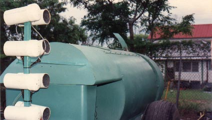
Figure 1 Tree-See on a Swanson sprayer (www.treesee.com)
This technology is still used today; Sensors detect specific zones on the canopy and actuate boom sections, or individual nozzles, to only spray the target zone. But optics and machine learning are evolving. Now they can modulate flow from individual nozzles in response to changes in canopy density. To be clear, that’s not just “on/off”, but variable flow.
Eventually, these systems will be able to identify and respond to specific pests (or pest damage) and adjust plant growth modifier rates based on canopy density or bloom counts. The possibilities are amazing. As an aside, interested readers can learn more about airblast sensors in this excellent article from Oregon State University which one of the authors later summarized for us here.
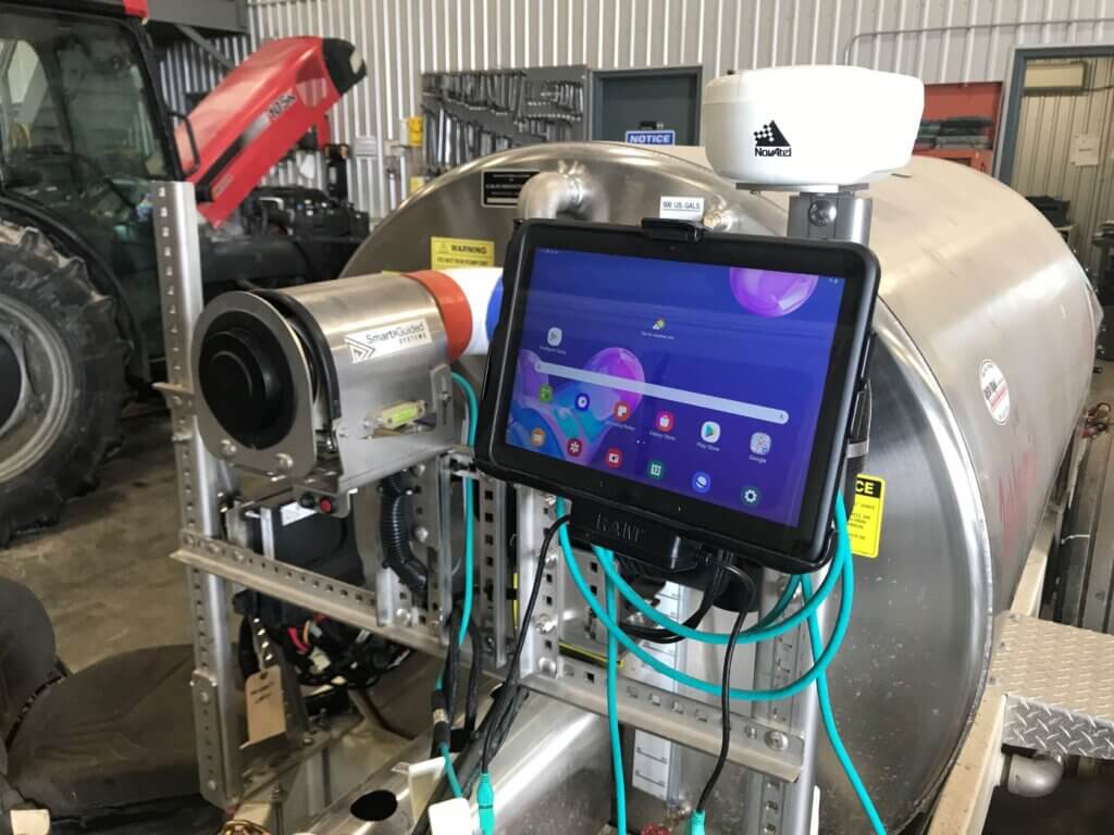
Figure 2 LiDAR and control interface for a Smart Apply system fitted to a Turbomist sprayer
However, as operators embrace this technology, they should be aware of the current limitations. Canopy-sensing optics are great at managing waste (their primary selling point seems to be pesticide savings), but this depends on crop morphology and planting architecture. It makes sense to not spray what isn’t there, but the gaps may not be as big as you think.
Non-continuous canopies require the spray to lead and lag to some extent before and after passing the target to ensure sufficient coverage. Given the difficulty inherent to spraying to the tops of tall canopies, some specialists believe the top nozzles should never disengage. And, in the case of uniform canopies that form continuous hedge-like rows, the potential savings is greatly reduced.
Further, all of these systems assume that application efficiency is primarily dependent on matching liquid flow rates to the profile (or perhaps density) of the target canopy. I don’t believe that’s true. At least, not entirely true. The impact of air settings on coverage efficiency and efficacy seems to have been marginalized.
For example, these sprayers do not account for the spray’s ability to span the distance from nozzle to target (i.e., transfer efficiency). That depends on the droplet size, sprayer air settings and the environmental conditions – none of which are monitored by sprayer optics. They also cannot “know” if the spray gets intercepted by the target (i.e., catch efficiency) or if it deposits a biologically-active residue on the target surface (i.e., retention). Droplets must be retained by the target surface and not bounce or run off.
What this means is that these sprayers, like any sprayer, can only promise “coverage potential”. Operators are still required to perform the following tasks:
Optimize air direction and air energy in relation to canopy size, travel speed and environmental conditions.
Use water-sensitive paper, or some other means of quantifying coverage, to ensure your target receives threshold coverage.
Monitor and adjust practices throughout the season in response to changing conditions.
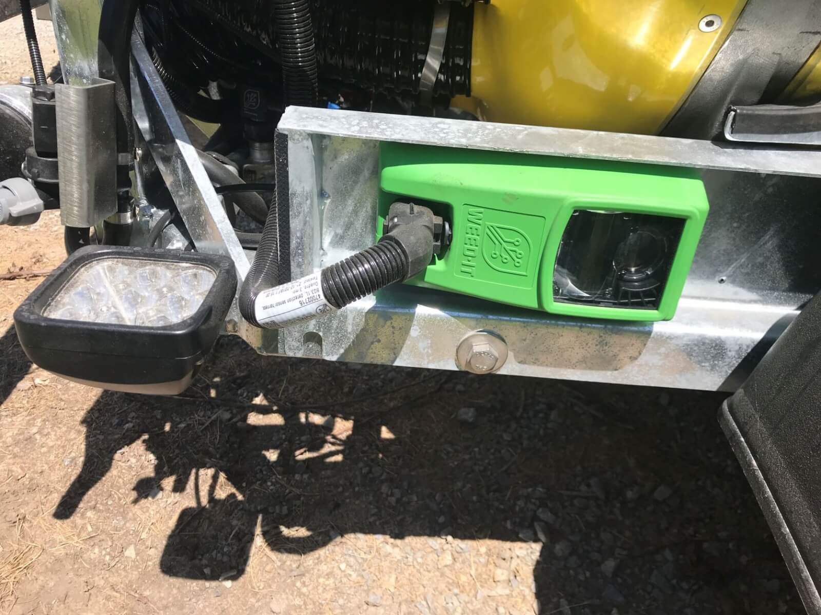
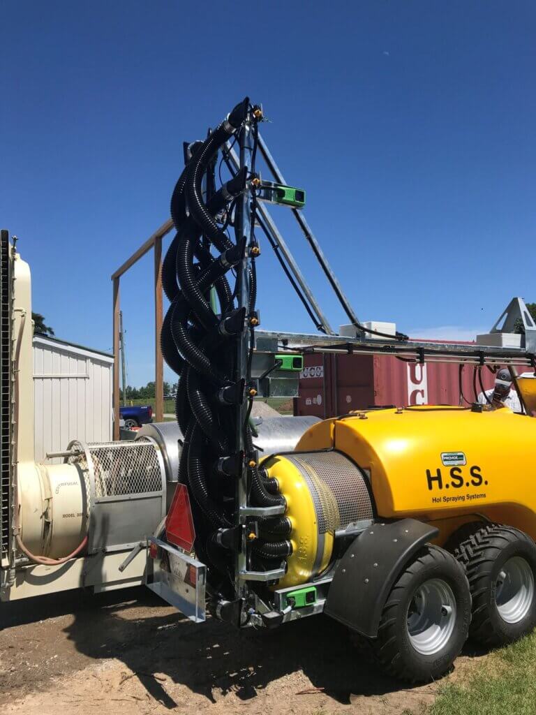
HOL’s Intelligent Spray Application (I.S.A.) system employing Weed-It sensors.
So what’s missing? How do we progress beyond what is arguably a sophisticated rate-controller?
In my opinion, I believe the pitcher needs a catcher – a closed-loop feedback system. Optics would identify the target, nozzle flow would respond, and then a digital spray sensor in the target canopy would detect and report coverage back to the sprayer so machine learning could make iterative adjustments in real-time.
Spray-sensors are not a new idea, as wetness-detection systems have been used in forestry since the 70s. But, a sensor that can discern spray coverage would yield far more detail, and once again it seems Ken Giles is a pioneer in this concept. Such a sensor, integrated with sprayer optics and machine learning, could summarily account for all the unknowns that interfere with spray from the moment it’s released to the point that it (hopefully) lands. That’s some serious crop-adapted spraying.
And yes, it would be fantastic if there were some manner of anemometer tied to a baffle or louvers in the spray head. Air energy could be balanced between up- and down-wind sides, and further adjusted to compensate for the distance to the canopy… but I’m dreaming in technicolour, now.
Until then, sprayer eyes can only blindly dictate the release of spray into the airstream based on an assumed coverage constant (e.g., 1.2 oz./ft3). It remains for the sprayer operator to act as the brain, optimizing sprayer settings, quantifying coverage, and making changes to reflect conditions.
Learn more about how to optimize the fit between your airblast sprayer and your target by downloading a free copy of our Airblast 101 textbook.
Calibration should be a regular practice for every operation that uses a sprayer. Part of that process is confirming that each nozzle is operating within the manufacturer’s specifications. This is a must for researchers that adhere to Good Laboratory Practices and for custom operators that sell their services. But we didn’t just fall off the turnip truck… we know nobody else does it. In fact, we’re surprised when we hear an operator HAS checked their nozzle flow.
And we get it. It can be awkward and time consuming. A field sprayer with 72 nozzle bodies and three nozzles in each position has a whopping 216 nozzles. A tower-style or wrap-around airblast sprayer has fewer nozzles, but the operator needs a ladder to reach them all and they don’t point straight down, so a tube must be used to guide the spray into a collection vessel.
And when pressed, any operator that does not regularly check their nozzles counters by saying “my tank empties in the same place every time, so why check them?” Even if the sprayer does start to go further on a tank, the operator can speed up or adjust the rate controller to drop the pressure a little.
Fair enough. This isn’t a hill we choose to die on.
But we will say that nozzles worn by even a few percent don’t only cause a change in flow rate, but may indicate a deteriorating spray quality and spray geometry. And, when one (or a few) nozzles are worn and others are not, it’s the same as when a single nozzle is plugged – the operator won’t be able to tell from the cab because the rate controller tends to mask the problem. And, if using PWM to apply a simultaneously reduced broadcast rate, perhaps the issue is amplified? All of this impacts coverage uniformity.
We’ll get off our soapbox now.
Over the years we’ve encountered many methods for determining a nozzle’s flow rate. We wanted to try each of them and characterize their accuracy, precision, time required, and ease of use. This is not a ranking where we wanted to find “The Best” method. The best method depends on your situation. If you’re a researcher, then accuracy and precision may trump time and expense. If you’re a custom applicator, then perhaps time is the critical factor. And if it’s your own operation, perhaps expense matters most. It’s up to you.
Method
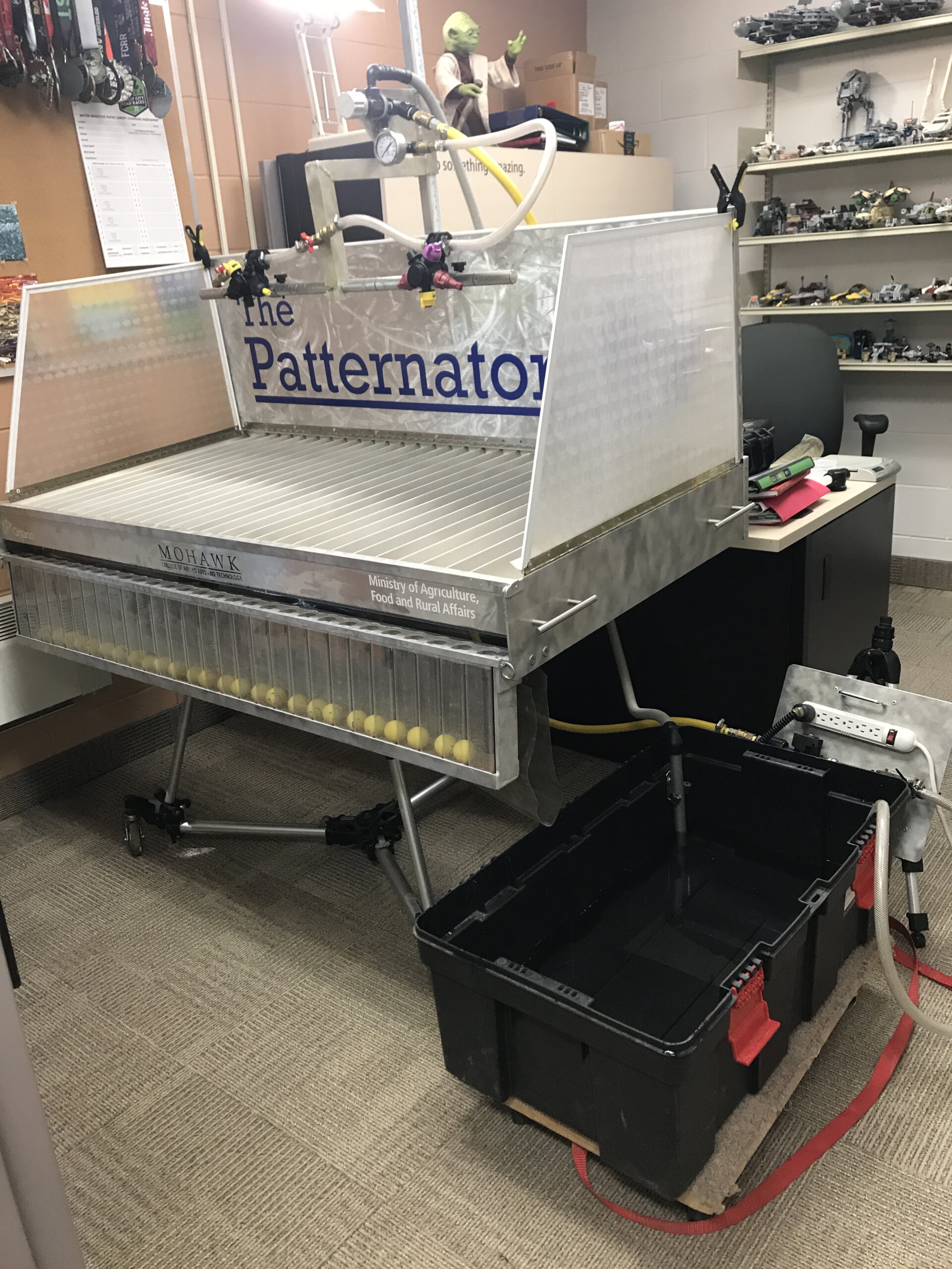
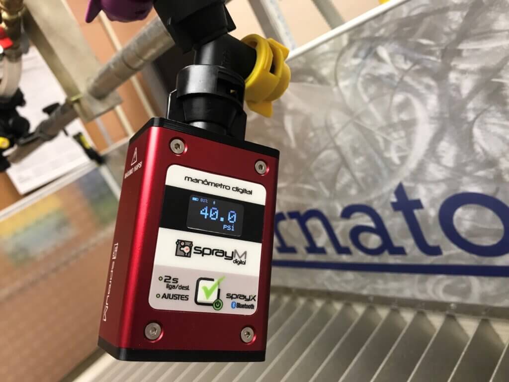
The following tests were performed on a spray patternator table. A single nozzle was operated by a ShurFlo 2088-594-154 positive displacement pump. Pressure was set using a bypass regulator and an analog pressure gauge, confirmed by a SprayX digital manometer positioned under the nozzle body via a splitter. Room temperature water was used.
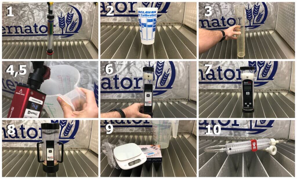
We tested ten nozzle flow rate measurement systems. There are others out there, but we limited the selection to farmer-oriented systems and not those used in mandatory government inspections.
Billericay Flowcheck
Delavan Calibration Cup
Graduated Cylinder
Greenleaf Calibration Pitcher
SprayX SprayFlow Turbo
SpotOn SC-1
SpotOn SC-2
SpotOn SC-4
Weighed Output
Lurmark McKenzie Calibrator
Three samples were taken from a new TeeJet XR8004 at ~40 psi and three samples taken from a new TeeJet AIXR11004 at ~70 psi. An exception was made for the Billericay Flowcheck which specified 43.5 psi (3 bar) for all sampling. All systems were emptied or dried as much as their design permitted between samples.
All data was converted to gallons per minute and the flow measured was compared to the calculated flow for the nozzle and pressure used. For example, if the manometer read 38 psi for the 8004, then the formula 0.4 x (38 psi ÷ 40) 0.5 gives us a calculated flow of 0.39 gpm. If the method reported 0.41 gpm, then it would be off by +5.1%.
Results
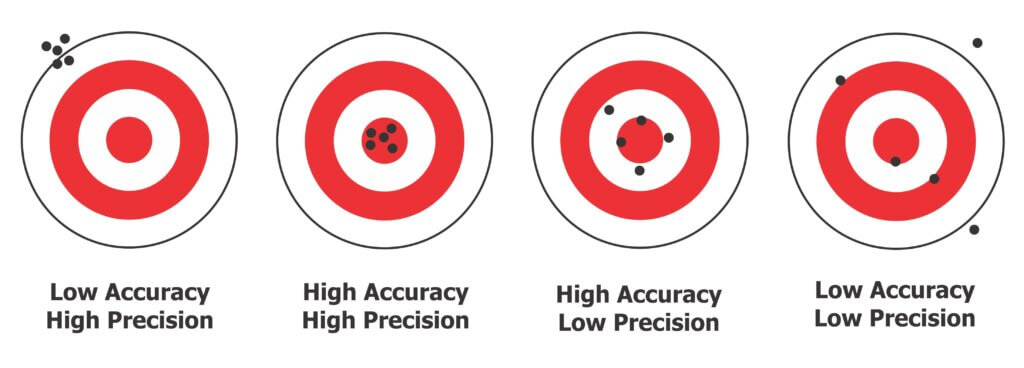
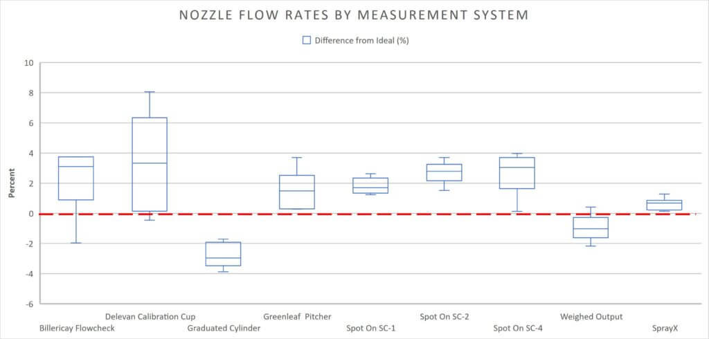
Consider the accuracy and the precision of each system when you review the results. Remember that precision means you get the same result with very little variation while accuracy means that on average you get the correct result. And, for context, remember that most recommend changing a nozzle when it is 10% more than the ideal flow rate. We prefer 5%, and if three or more nozzles are off spec, replace them all as a batch because they’re likely all very close. Compared to most spraying costs, a set of nozzles is not worth quibbling about. Some operators just change them annually and don’t bother with testing at all.
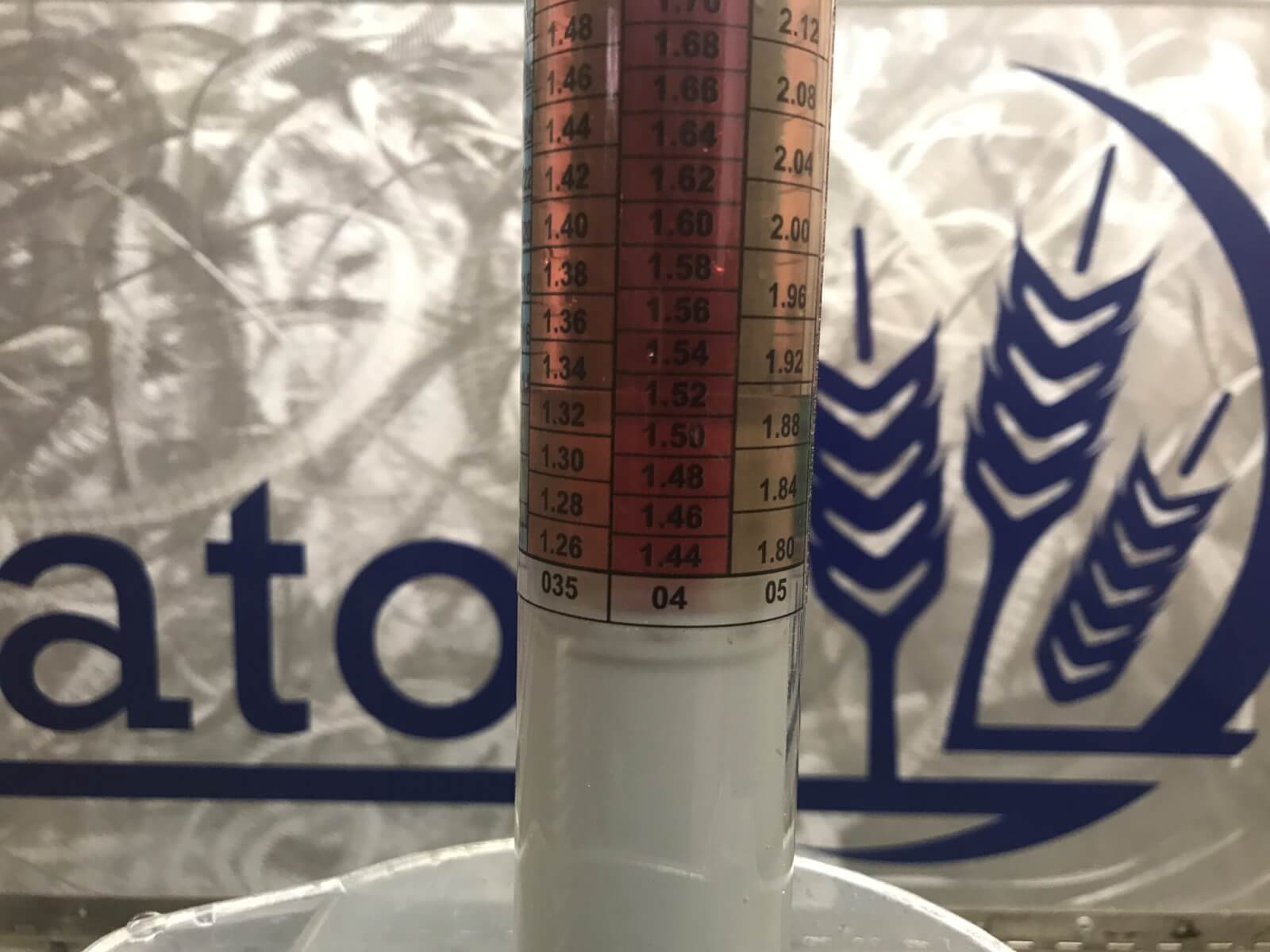
Billericay Flowcheck: This is a passive measurement system. You must select the nozzle size on the bottom of the collector and suspend the unit from the nozzle body. It’s designed for a horizontal boom and you’d have trouble using it with any other sprayer. You also have to set the pressure to exactly 43.5 psi (3 bar). While fairly accurate, it spanned about +/-2.5% off ideal. You have to read from the right scale, which in this case was red and rather difficult to read because of the low contrast. It took about two minutes to reach equilibrium for each reading and a lot of liquid is lost during the process.
We attempted to keep the unit plumb so the meniscus and scale aligned correctly. We found it difficult to read the ’04 scale because of low contrast. Pictured is 1.53 lpm.
Delavan Calibration Cup: This small, one-handed plastic cup had a scale printed on the outside. We were limited to a 15 second collection because of how quickly it filled. Some spray was lost to mist and bounce and we used the “Fluid Oz” scale to get the highest resolution from the measurement. It took less than a minute to collect and read from the cup, but had the lowest precision and accuracy.
Graduated Cylinder: There was little or no mist or bounce from escaping spray during collection. Our 1,000 ml graduated cylinder took 30 seconds at 40 psi and 20 seconds at 70 psi to fill making it roughly one minute per reading. A few light taps removed bubbles and once the liquid settled we could read the level. This must be performed on a level surface (in our case we used the digital level app on our iPhone). This was a very precise method, varying by less than 2%, but it wasn’t very accurate. We may have introduced error when reading the meniscus (always read from the centre) or perhaps the plastic distorted over time and affected accuracy. It may be difficult for most people to get a high quality, scientific-grade graduated cylinder.
Greenleaf Calibration Pitcher: The pitcher had multiple scales but once again we used fluid ounces because it had the highest resolution. With the highest capacity, we were able to collect for an entire minute. Despite holding the vessel at different angles and distances, we lost a lot of spray to mist and bounce and the nozzle body was beaded with water at the end of each trial. After tapping the vessel to remove bubbles and reading on a level surface, it took about 1.5 minutes per sample and averaged an average 3% more than the calculated ideal flow rate.
Innoquest Spot On Digital Calibrator: We’ll discuss all three Spot Ons together. The Spot Ons were a game-changer in North America when they first came out. You can read a peer-reviewed article about the SC-1 by Dr. Bob Wolf et al. published in 2015 in the Journal of Pesticide Safety here. The SC-2 is a new version of the SC-1 with added digital features that allow the user to calculate gallons per acre and it indicates tip wear based on the 10% industry standard . The most important improvements were a reduced sensitivity to foam and a thicker foam diffuser to reduce the chance of errors. The SC-4 works exactly like the SC-1, but has a larger capacity intended for high flow rate nozzles (e.g. hollow cones on an airblast sprayer). In each case, the Spot On will report in several units, and must be held steady under the nozzle flow (i.e. not moved during reading). The SC-1 and 2 took less than 12 seconds for each reading and the SC-4 took closer to 30. The SC-1 and SC-2 were relatively precise but read consistently higher than the calculated flow rate. This may be an artefact given that the units only read to 2 decimal places and this may have exaggerated any error. The SC-4 was the least accurate and precise of the three. The Spot Ons were the fastest and easiest to read of the methods used.
Weighed Output: This method is based on the fact that 1 ml of water weighs one gram. Spray was collected for 30 seconds and weighed on a new, $25 CAD digital kitchen scale, which was tared (i.e. the weight of the vessel subtracted from the overall weight). While subject to errors from manual timing, it has the merit of removing the challenge of reading a meniscus and it’s relatively inexpensive. This method was precise and relatively accurate compared to the other methods used. It took about a minute per sample.
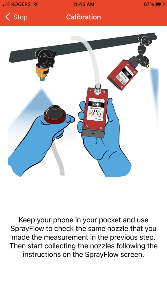
SprayX SprayFlow Turbo: This was the most sophisticated method we used. The kit comes with a digital manometer, a flowmeter and a digital scale. It works though a smartphone app (screenshot below). You first have to set up a virtual sprayer, informing the app how many sections and nozzles will be tested. Then you must calibrate the flow sensor by taking three measurements versus a weighed output to eliminate possible variations caused by the nozzle, pressure, temperature, and the density of the liquid. The app walks the user through each step. This method took the most time to set up (easily 10 minutes). However, once it was set up, each nozzle could be tested in less than 30 seconds apiece. This method was the most accurate and precise, but the price may place it out of reach for the typical user.
Screenshot from the SprayX SprayFlow app.
Lurmark McKenzie Calibrator: This method is not reported in the box-and-whisker plot because there were significant problems that prevented accurate readings. It was difficult to get a seal over the nozzle and the floater ball would either stick or fluctuate. After several attempts, this method was abandoned.
Conclusion
In order to test if a process, or a thing, is occurring or produced within acceptable limits, we need a detection system with a high enough resolution. In manufacturing (e.g. factory production) this is an essential requirement in quality assurance. Let’s consider a +10% deviation from the nozzle’s ideal flow rate to be our indication that a nozzle needs to be replaced. We need a measurement system with an appropriate scale and one with sufficient precision to ensure we don’t get a false reading. Based on our data, I would suggest all systems reviewed, save the measurement cup, are viable. Even if we elect to use a more stringent rejection threshold of 5%, some systems are more precise than others (i.e. less variability), but all but the cup should still be sufficient.
What’s the penalty for not testing, assuming we’re not talking about significantly deviant nozzles? Let’s say, for example, we are not using a rate controller and we are applying 20 US gpa at 12 mph using 72 nozzles on 20″ centres. Our boom would have to spray 58.2 gpm, which means each nozzle would have to emit 0.81 gpm. If those nozzles sprayed 5% more than intended, we’d be spraying 21 gpa instead of 20 gpa. That means for a 1,200 gallon sprayer, you’d do 57 acres instead of 60. We would have the same result if we dropped from 12 mph to 11.45 mph, which is about 5% slower. Maybe that’s a big deal for your operation, or maybe not. For most, 5% is well within the typical error inherent to spraying. Then again, perhaps it’s more important to know that each nozzle is performing in a manner similar to its neighbours to ensure the highest degree of coverage uniformity.
Ultimately, it is important to ensure you’re as efficient as possible, and that means understanding what your nozzles are doing so you can decide if-and-when it’s time to replace them. Pick whichever method makes it easiest for you to justify testing your nozzles and do it at least once a year when you take your sprayer out of long term storage.
Thanks to all the companies that donated or loaned their calibrators to make this article possible.
In 1977, David Shelton and Kenneth Von Bargen (University of Nebraska) published an article called “10-1977 CC279 Gear Up – Throttle Down”. It described the merits of reducing tractor rpm’s for trailed implements that didn’t need 540 rpm to operate. In 2001 (republished in 2009), Robert Grisso (Extension Engineer with Virginia Cooperative Extension) described the same fuel-saving practice. Again, it was noted that many PTO-driven farm implements don’t need full tractor power, so why waste the fuel? He tested shifting to a higher tractor gear and slowing engine speed to maintain the desired ground speed. 700 diesel tractors were tested, and as long as the equipment could operate at a lower PTO speed and the tractor itself didn’t lug (i.e. overload), as much as 40% of the diesel was saved.
How this applies to Airblast
For airblast operators with PTO-driven sprayers and positive-displacement pumps, this has potential for reducing air energy. Gearing up and throttling down (GUTD) sees the operator reducing the PTO speed from 540 rpm to somewhere between 350-375 rpms, which not only saves fuel but more importantly slows the fan speed. This may be an option when air energy from the sprayer, even at higher travel speeds and a low fan gear, still overblows the target canopy.
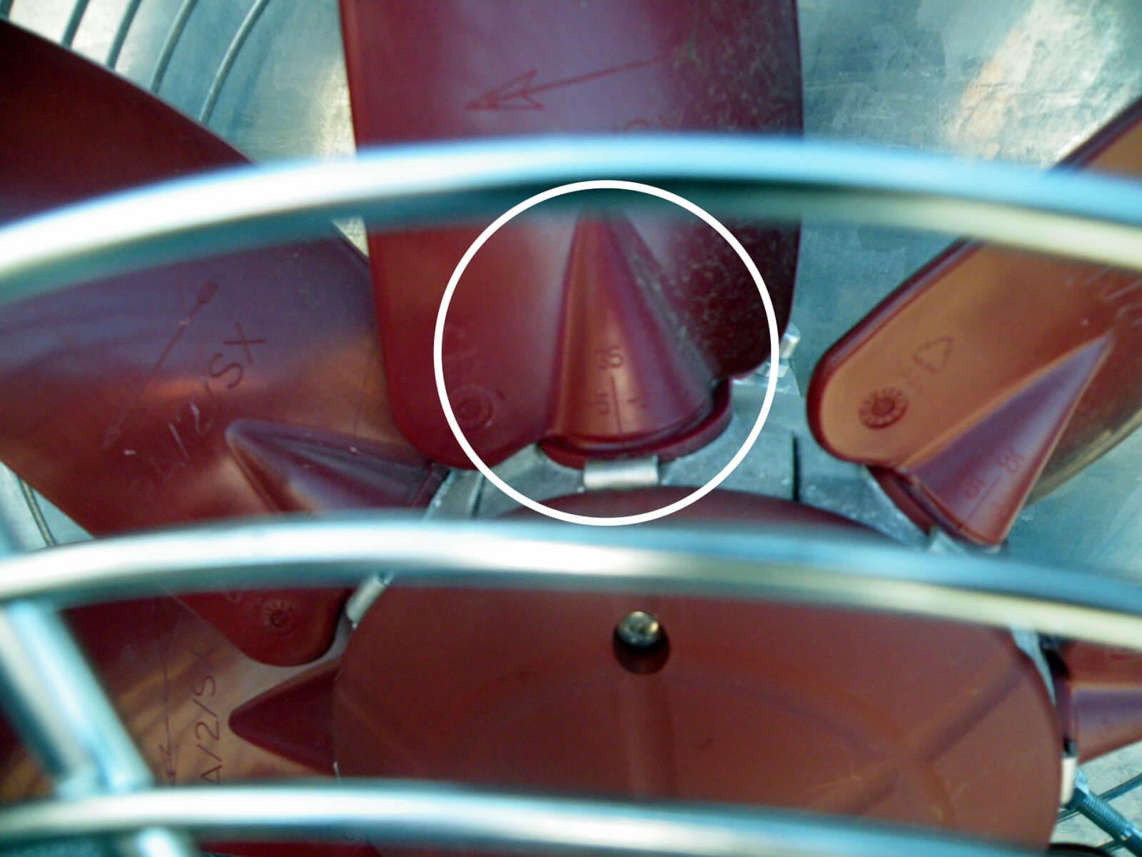
Some airblast sprayers, like this one, feature fan blades with manually-adjustable pitch to increase or lower air volume and speed. It’s often a pain to try to adjust them, and most operators only try it once.
A good time to try this out is early in the spraying season when (most) canopies are dormant and at their most sparse. For example, when applying dormant sprays in apple orchards, look to see if the wood on the sprayer-side gets wet, but does not creep around the sides. This suggests that the air, and much of it’s droplet payload, are being deflected. When the air speed is slowed, it will become more diffuse and turbulent on target surfaces, and this turbulence helps more droplets deposit in a panoramic fashion within (not past) the target canopy. Look to see if the wood is wet >50% around the circumference of the branches. You’ll get the rest when you spray form the other side.
Limitations
GUTD is not always appropriate. It requires airblast sprayers with PTO-driven positive displacement pumps (e.g. diaphragm). Airblast sprayers with centrifugal pumps would experience a drop in operating pressure and would have to be re-nozzled. Further, the pump must have sufficient surplus capacity to maintain pressure at low rpms.
GUTD is not intended for air-shear sprayers that employ twin-fluid nozzles because dropping air speed below a certain threshold may compromise spray quality; the air needs to be fast enough to create and direct spray droplets
The tractor must have sufficient horsepower (more than 25% in excess of minimally-required capacity) to permit the reduction in engine torque. This is especially important if the operator is on hilly terrain. If the tractor begins to lug (e.g. black smoke, sluggish response, strange sounds) you’ll be in trouble.
Observations
We first experimented with GUTD in 2013. We noticed how much quieter the sprayer was, and the fuel consumption was certainly reduced. One grower-cooperator switched to a GUTD spray strategy mid-way through their dormant oil application in pears. We saw the trees immediately began to drip. Panoramic coverage was improved significantly; once the operator passed down the other side of the target, capillary action and surface tension helped to give near-complete coverage.
However, in one instance, the operator was already applying a low spray volume per hectare using air induction nozzles and their lowest fan gear. By further slowing fan speed using GUTD, coverage at the top of his cherry trees was compromised.
In short, GUTD can work under the right circumstances. If you want to try it, use water-sensitive paper to establish a base-line with your current practice, and then evaluate coverage after you change your sprayer settings.
The Fundamental Relationship, a concept by Professor D. Ken Giles (Emeritus), UC Davis Biological and Agricultural Engineering Department, is a way of talking about calibration without numbers and formulas. It is valuable for teaching concepts important to calibration. Since it is a relationship, it describes the variables needed and how they relate to each other.
We see here that land rate is inversely proportional to application rate. Thus, when land rate (either speed or swath width or both) are increased (and no other factors change), application rate is decreased. Likewise, flow rate is directly proportional to application rate. Thus, when flow rate is increased (and no other factors change), application rate is also increased. When flow rate is decreased (and no other factors change), application rate is also decreased.
The Fundamental Relationship is also a good way to do the math of calibration because nothing needs to be memorized. As long as the units are checked, you can’t go wrong. The Fundamental Relationship works for any sprayer calibration, as long as the units are tracked correctly and the flow rate correlates to the land rate, i.e., the land rate used is the swath that the nozzles (flow rate) are covering.
So, if the flow rate (GPM) used in the formula is for ½ of an airblast set up, the swath width in the land rate calculation would be ½ of the row width. If, for example, it is for a weed sprayer with 2 nozzles, the swath width would be the width the 2 nozzles are covering. Remember to think about this as what area is being covered by the spray:
Flow rate units are straight forward: gallons/minute.
Land rate can be a bit tricky because no one thinks in terms of acres covered per minute.
Land rate is tractor speed × swath width covered by the nozzles used to calculate flow rate.
Land rate in the above needs to be calculated in the units “ac/min”. Since there are 43,560 ft2 in an acre, the easiest way to calculate is to use the swath width in feet, and the speed in ft/min. Multiplied, this then will give you land rate in ft2/min, which can then be converted to ac/min.
Using MPH as Speed
When you measure speed in the field, those who have a speedometer on their tractor will tell you their speed in MPH. To go from a land rate with speed as MPH to ac/min, the following unit conversion is used when multiplying the speed in MPH times the swath width in feet:
Note: speed should always be measured and verified. Speedometers are notoriously incorrect!
Calculating nozzle flow rate (GPM):
You can also use the Fundamental Relationship to calculate the flow rate needed for a desired spray volume (application rate) when you have a set land rate (speed and swath width). This is necessary to help you choose your nozzles. Tractor speed is first determined by checking the coverage-using water sensitive paper or another coverage indicator like kaolin clay, and the fan (using ribbons in the canopy), to go as fast as safely possible while still getting adequate coverage. Swath width for any given field is set. What is left then is to calculate the GPM needed to achieve that application rate at that speed and swath width. This will allow you to select your nozzles based on individual nozzle GPM for a certain pressure.
To get the required GPM for one side of the sprayer, you multiply by ½:
GPM (one side of sprayer) = GPA × [(Miles/Hour × swath width (ft)) ÷ 495]× 1/2
GPM (one side of sprayer) = GPA × [(Miles/Hour × swath width (ft)) ÷ 495]
I’ve seen some folks round up the 990 to 1,000, which makes the above formula easier to remember.
Why I think the “495 formula” is bad for calibration
In my experience of teaching calibration math, folks often want to fall back on the formula they have used instead of trying the Fundamental Relationship. The problem I have with the “495 or 990” formulae, is that with using ground speed in MPH, often the step of measuring speed, a critical step for optimizing spray coverage, is eliminated.
Ground speed is assumed, the speedometer is assumed to be correct, and the entire step of measuring and setting speed is omitted-big mistake! Setting speed using flagging tape in the canopy and looking at the “Fan : Speed : Canopy” interaction is probably the most important step of calibration and optimizing coverage. So, if you must use the “495 formula”, please actually measure your ground speed!
Measuring speed manually
Typically, at least 100 feet are marked off to measure actual speed with a stopwatch. If you measure actual tractor travel time for a 100 foot length, you will likely find most common spraying speeds are timed in seconds. These can be converted to minutes, and then used in the formula for speed as ft/min which is then multiplied by the swath (or row) width in feet to obtain ft2/min, which can then be converted to ac/min.
If swath width is 6 feet, the land rate (or area the nozzles are covering) is calculated as:
264 ft/min × 6 ft = 1,584 ft2/min
In acres covered per minute, we divide by 43,560 ft2/ac to obtain a land rate of 0.036 ac/min. To travel 100 feet at this speed, it takes 0.37 minutes or 22.7 seconds. So, it is not uncommon to time 100-foot tractor runs in 21-23 seconds (which is why you need a good stopwatch). These runs are best done on the type of terrain to be sprayed; and it’s always good to take several times and average.
Remember that the speed is written as distance travelled/time. Sometimes when measuring speed, I’ve noticed that it will be written as time/distance travelled, which gives the wrong number. Track units!
Establishing an airblast nozzling solution is an involved process. We must first define the working parameters and flush out any special circumstances. Then we use an iterative approach to identify suitable nozzle combinations that require minimal changes to the sprayer.
This article outlines my process step-by-step and then applies it to a hypothetical orchard scenario. If readers wish to delve deeper into the variables or the reasoning, several links to supporting articles are provided. Be aware that nozzling the sprayer is the penultimate step in establishing optimal sprayer settings. Operators should first adjust air settings, which includes identifying a suitable travel speed. The last step in setting up any sprayer is to verify you are achieving threshold spray coverage.
Step One: Establish sprayer parameters
Is there more than one sprayer available? In diverse plantings, it may be more efficient to assign a sprayer to blocks that require the same nozzling solution.
How many nozzle positions are there on one side of the sprayer? If the nozzle bodies are roll-over style the operator can alternate between two different nozzles in each position. Some designs have twice as many nozzle bodies as needed. The intent is to assign two unique nozzle solutions in an alternating A-B set-up. This additional capacity gives us some flexibility if needed.
Is this a tower or a low-profile axial sprayer? Generally, we distribute nozzle flow evenly over a tower boom but distribute ½ the flow in the top 1/3 of the boom on a low-profile axial sprayer (depending on canopy shape and density). Air-shear and one-sided sprayers are special cases that are not addressed in this article.
What is the average travel speed, and can the operator easily change it? This process assumes the selected speed achieves a reasonable work rate while optimizing the interaction between sprayer air and the canopy.
What is the average operating pressure, and can the operator easily change it? For sprayers with positive displacement pumps, pressure is easily changed via the regulator. Not so for sprayers with centrifugal pumps. Pressure-based rate controllersempower an operator to dial in their desired volume and are easiest of all .
Step Two: Establish target parameters
What is the row spacing (or spacings)? Some operations include a variety of canopy morphologies and planting architectures.
What is the target volume (or volumes)? Operators often use a range of volumes to reflect the product being applied and the canopy area-density. This process assumes the volume will provide threshold, uniform coverage without misses or excess.
Step Three: Are there any environmental, geographical or adjacency concerns?
Each operation is unique, including conditions that may influence nozzling. For example, open water, sensitive crops, or residential areas adjacent and downwind of the planting may warrant drift-reducing nozzles or require the operator to only spray inward from one side of the sprayer. In another example, dry and windy conditions may require nozzles that produce a coarser spray quality will improve their survivability. Rolling hills and uneven alleys may cause sway that prevents the upper-most nozzles from consistently reaching the target.
Step Four: Find out why the operator is re-nozzling
The answer may reveal the operator’s willingness and ability to make changes to sprayer settings. For example, if their objective is to improve the match between sprayer and canopy it implies a willingness to take a more active role in spraying. Conversely, a less experienced operator might be satisfied with a more robust (i.e., wasteful) set up that does not require many changes between blocks.
Step Five: Determine the highest and lowest boom flow requirements
The following formulae relate travel speed, row spacing, and the desired volume sprayed per planted area to the output from a single boom. I recommend downloading this Excel-based calculator to make the process easier.
US Imperial Formula Output from single boom (gpm) = [(Sprayer Output (gpa) × Travel Speed (mph)) ÷ 990] × Row Spacing (ft)
Metric Formula Output from single boom (L/min) = [(Sprayer Output (L/ha) × Travel Speed (km/h)) ÷ 1,220] × Row Spacing (m)
Using the formula with the appropriate units, enter the highest desired volume, the fastest travel speed and the longest row spacing. This will give the highest rate of flow the boom must satisfy.
Repeat this process using the lowest desired volume, the slowest travel speed and the shortest row spacing. This will give the lowest rate of flow the boom must satisfy.
The ultimate objective is to select a combination of nozzles that can produce these two flows, distributed sensibly along the boom, with no gaps or excessive flow relative to the target. Ideally, the operator should be able to alternate between these two flows with as few changes as possible.
Step Six: Satisfy the highest flow
This step requires a nozzle manufacturer’s catalogue and a calculator (or the downloaded Excel spreadsheet). We must assume the range of available nozzle positions are oriented to span the target canopy with no over- or under-spray.
Divide the highest flow requirement by the number of available nozzles. Hypothetically, a nozzle size that produces this flow would satisfy the highest flow requirement while providing an even distribution along the boom.
Using the nozzle manufacturer’s catalog, find the flow table for the nozzle you want. Generally, a molded hollow cone nozzle is the preferred choice (e.g., TeeJet’s TXR ConeJet or Albuz’s ATR). If drift is a concern, there are also air induction (AI) hollow cones available. AI nozzles are most effective in the top two or three nozzle positions where drift potential is highest. However, they may require higher flow than calculated to compensate for a reduced droplet count.
Find the operating pressure (it may be in either the column or row heading) and find a flow rate in the body of the table that is as close as possible to your calculated ideal. It’s almost never an exact match, so choose the option that is less than the target rate – not higher.
Imagine placing that nozzle in every available position. Add up all the rates to determine how close you are to the ideal flow. It will likely be less. To compensate, replace the top nozzle on the boom with a higher rate and re-calculate the total flow. Repeat this process, substituting for nozzles with a higher rate, moving top-down along the boom until the flows match.
You have now satisfied the demand for the highest flow.
It is important to note that this process assumes the flow distribution along the boom should be relatively even, perhaps skewed towards the top. However, it is sometimes appropriate to distribute the flow differently to reflect each nozzle’s distance-to-target and the density of the corresponding portion of canopy it needs to spray. This tends to be the case when pairing low-profile radial sprayers with large or trellised canopies, and you can read more about that process in this article.
Step Seven: Satisfy the lowest flow
This is the art-and-compromise part of the nozzling process.
Confirm that the range of available nozzle positions still corresponds to the target. Quite often, the lowest flow is intended for smaller canopies. If so, we may no longer have as many nozzle positions to work with.
Imagine the sprayer is still nozzled for the highest flow per the last step. Leaving the highest effective nozzle on, imagine turning off every second nozzle. Add up the flows and determine how close you are to the lowest rate of flow. It is often still too much. Do not turn off any more nozzles or you may create gaps in the swath.
Instead, return to the nozzle catalogue and re-calculate the flows for the same nozzles, but using a lower operating pressure. Can you make that work? If not, you may have to go back further in the calculation (Step five) and recalculate the lowest flow required using a faster travel speed. This will reduce the demand for flow.
If none of those options are viable you will have to consider re-nozzling. Perhaps that’s swapping a few nozzles to lower rates. Hopefully this only requires the operator to flip a roll-over position, but it may mean using a wrench to remove caps and swap nozzles.
Once you’ve satisfied the lowest flow, the hardest part of the process is complete.
Step Eight: Satisfy the other permutations
The last step is no different than what we’ve already done. Go back to Step Five and calculate the flow for each spraying situation. That is, each unique combination of row spacing, travel speed and target volume. Using the nozzles already on the sprayer, adjust the pattern of nozzles in use (and pressure and/or travel speed if required) until each unique flow requirement is satisfied.
Step Nine: Record the setups, nozzle the sprayer and test the coverage
Be sure to clearly record the sprayer settings required to achieve each flow. Purchase the nozzles and take the time to test each set up using water sensitive paper to ensure coverage is achieved.
A working example
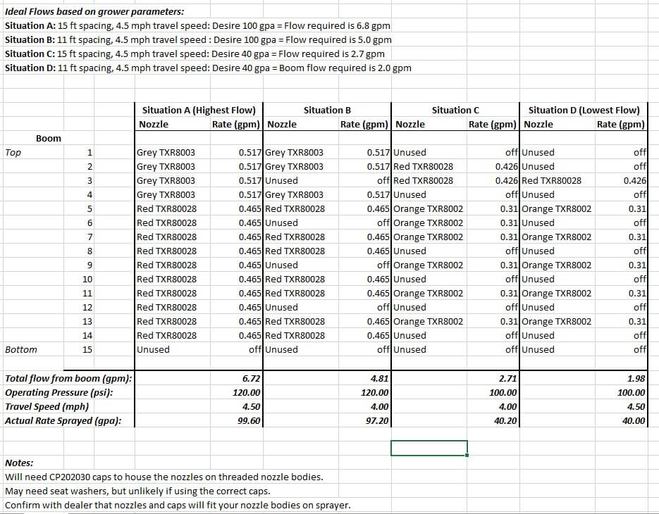
Let’s apply this process in a hypothetical orchard. I’ve included a screenshot of the spreadsheet I use to record the final nozzling solution (below) but feel free to design your own. It includes the nozzling solution for this example.
Our orchard is a 50 acre operation with both 11 and 15 foot row spacings. They have one tower sprayer with 15 nozzle positions on one side and they are not roll-over bodies. The operator wants to apply a 40 gpa volume (concentrated) and a 100 gpa volume (dilute). Their preferred travel speed is 4.5 mph and preferred operating pressure is 140 psi, but they are willing to change them if required.
We use the Excel calculator to work out the ideal highest and lowest demands for flow:
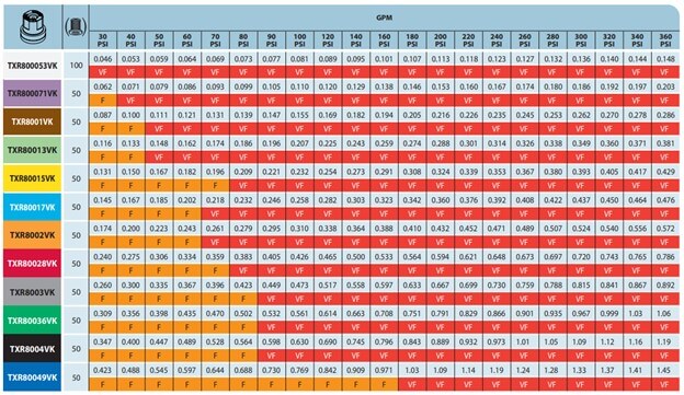
I usually shut off the lowest nozzle position because it almost never aims at the target. Let’s divide the high flow of 6.8 gpm by 14 available positions to give us an average output of 0.48 gpm per nozzle. This operator wants to use TeeJet TXRs, so using their table (below) we see that at 140 psi the Orange ’02 is too low and the Red ‘028 is too large. If we drop the operating pressure to 120 psi, the Red ‘028 is much closer at 0.465 gpm, so let’s do that.
A quick check gives us our current boom flow: 14 positions × 0.465 gpm per nozzle is 6.51 gpm of boom flow. We wanted 6.8 gpm, so let’s go up to the Grey ’03 in the top three positions. Now it’s 4 × 0.517 gpm + 10 × 0.465 gpm = 6.72 gpm. That’s close to our ideal 6.8 gpm, so let’s lock that down. If you want to see what this is in gpa, you can plug the value into the Excel calculator to discover it’s 99.6 gpa. Pretty darn close to our target 100 gpa.
Now using that nozzling arrangement, let’s see if we can satisfy the lowest flow requirement by shutting off every second nozzle position, leaving the highest position on. Doing so reduces us to two Greys and five Reds, totaling 3.36 gpm. That boom flow is much too high compared to the 2.0 gpm we need. However, in our hypothetical orchard, this block has shorter trees so we don’t need the highest nozzle. That drops us to only one Grey and a new total of 2.84 gpm. Good try, but it’s still too much.
Let’s reduce the operating pressure from 120 psi to 100 psi, which is as low as I like to go. According to TeeJet’s table, the Grey produces 0.473 gpm and the Red produces 0.426 gpm at this pressure. This gives us a new total of 2.60 gpm. Still too high! Well, let’s raise our travel speed from 4.5 mph to 5.0 mph and recalculate the lowest flow for Situation D:
This still won’t do it, and driving that fast (even if it’s possible) would change our air settings too drastically. Having exhausted all the easy options we have no choice but to re-nozzle the sprayer for the original lowest flow requirement.
Returning to the TeeJet table we see the best fit is to spray at 100 psi using one Red TXR80028 and five Orange TXR8002s. It’s a lucky break that our 1.98 gpm has come so close to the 2.0 gpm of flow we wanted.
Now let’s work out the best arrangement for the other permutations, Situation B and C. We need 5.0 gpm and 2.7 gpm, respectively. For Situation B, let’s use the nozzling solution from Situation A. We see that shutting off four nozzles gets us very close at 4.81 gpm or 97.3 gpa where we wanted 100 gpa. As for Situation C, let’s work from the nozzling for situation D. By adding a few more nozzles from that set, we can manage 2.71 gpm or 40.2 gpa.
Finally, we record all the settings (refer back to the spreadsheet image). We will need four Grey TXR8003s, ten Red TXR80028s and six Orange TX8002s per side, so 40 nozzles in total (plus a few spares for each rate). We will need to spray at 120 psi for Situation A and be prepared to shut off a few nozzles for Situation B. Situation C will require 100 psi and an entirely different nozzling and we will have to shut a few of them off for Situation D. Not only have we determined a nozzling solution, but we have revealed an efficient order for spraying the blocks that will require as little manual change to the sprayer as possible.
Summary
There is no one right answer to the question “which nozzles do I need” but there are certainly wrong answers. Bear this in mind when you buy a sprayer and the dealer offers you a factory-standard nozzle setup. Apply this process to your operation and be sure to use water sensitive paper to confirm the coverage and to make informed changes where required.